A Markov-modulated tree-based gradient boosting model for auto-insurance risk premium pricing

Abstract

In most sub Saharan African countries,the mechanism for pricing auto-insurance policies is tariff based. This means that the key factor that influences price changes is usually based on regulation and legislative dynamics. Additionally, where ratemaking is risk based, analysis has in most cases focused on internal historical data or claims history, particularly in the sub Saharran Africa. These policy regimes have led to unfair price distortions among policyholders and have increased risk of portfolios for most insurance companies. In this study we consider geographical location risk that influence auto-insurance claim process for an insurance company. The study develops a Markov-modulated tree-based gradient boosting (MMGB) model for pricing auto-insurance premiums. The Markov-modulated tree-based gradient boosting model is a Tweedie general linear model (GLM) based pricing algorithm with a compound Poisson-Gamma distribution whose rate varies according to accident risk in a Markovian process. Thus, the study extends the existing premium pricing framework by integrating a geographical location risk factor into the main pricing framework. The study applies the model to a motor insurance data set from Ghana. The results show that the proposed method is superior to other competing models because it generates relatively fair premium predictions for the non-life auto-insurance companies, helping to mitigate more the insured risk for the firm and the industry.

Keywords

Auto-insurance models Markov-modulated pricing gradient boosting risk premium pricing in Ghana

1. Introduction

The operational process of non-life Insurance assumes different risks profiles for the insured influenced by instabilities within the business environment. Predicting the financial obligation for claims in non-life insurance is quite complicated and usually depends on the structure of insurers liabilities. The question has always been how much premium to allocate to a policyholder to ensure fairness on the part of the insured and to avoid bankruptcy on the part of the insurer. The most critical task in insurance pricing is how to accurately predict the risk of claim and the expected coverage for the insured should the event occurs. The task of modeling claims has been a major challenge because of data structure which is usually highly skewed with many zeroes as well as high claim severity. Traditional modelling technique such as generalized linear modeling (GLM) technique as proposed by Nelder and Wedderburn [28] has been the major tool used for loss cost modelling (McCullagh and Nelder [24]). To cite few examples Haberman and Renshaw [19] and Mihaela [27] analyzed claims severity and frequency using the GLM technique. Smyth and Jorgensen (2002) also published a paper that used Tweedie GLM as an alternative approach in modelling claim frequency and severity. This modelling framework assumes that claims arrival has a Poisson distribution and claim severity follows a gamma distribution such that the total claim structure could be modelled with Tweedie compound Poisson. Even though Tweedie GLM is often used, it has a major drawback. One major drawback is that link between the variate and covariates which is usually constrained to a linear form is rare in practice. For instance, in auto-insurance, risk of claim is not necessary inversely related with age (McCartt et al. [25] and Anstey et al. [2]). To correct this draw back various procedures have been proposed. Wood [35] for instance proposed Generalized Additive Models (GAM) to overcome some of the deficiencies of the GLM such as the linear link to a more general form. However, with GAM the structure of the model must be specified. The main and interaction effects have to be specified by the researcher. This often result in specification bias which likely affects the predictive power.

To overcome the deficiencies of GAM, Yang, Qian and Zou [36] proposed a gradient tree-boosting algorithm for fitting compound Poisson models nonparametrically. Despite its strong predictive power, its outcome depends on the data generating process and the associated variables. The result of the literature reviewed showed a wide range of models that consider historical risk as the only basis for price differentiation among policy holders. However, the difference with this study is that we present a process of integrating location risk in the pricing framework. We utilized the concept of Markov chain and tree-based gradient boosting mechanism to derive the model instead of a single model that characterize most claim cost modelling by most researchers. This study seeks to improve on the work of Yang et al. [36] by obtaining an auxiliary variate x _i closely related to and has a positive correlation with the study variable, claims y _i.

The fast-paced changes in business environment and technological advancement require that we have an all-inclusive dynamic risk treatment, especially in non-life insurance. As cited in Djuric [8], Cramer [5] said that the goal of risk theory is to provide a mathematical analysis of the fluctuations in the insurance business and to suggest various means of protection against their adverse effects. This motive is what this study seeks to achieve. The rest of the paper is organised as follows, Section 2 presents methods and materials of the study, Section 3 also presents analysis and results of the two datasets employed and Section 4 presents the conclusion and recommendations of the study.

2. Methods and materials

2.1. Gradient boosting and predictive modelling

To keep the paper self-contained, we briefly explain the principles of gradient boosting, which is a statistical learning framework for predictive modelling. Gradient boosting is a nonparametric prediction framework that combines base(weak) learners into a strong predictive function in an iterative fashion. The idea originated from Breiman (1998) with further significant improvement by Friedman [15,16], Hastie, Friedman and Tibshiran [20] and Yang, Quian and Zou [36]. We briefly explain the general procedures for gradient boosting. Let x = (x ₁, x ₂, …, x _p)^T, be p-dimensional predictor variables and y a one dimensional outcome variable. The goal in predictive modeling is to determine the optimal function that maps x to y. This is done by minimizing the expected value of a loss function 𝜑(⋅, ⋅) over the function class ${\mathcal{F}}$ : $\begin{eqnarray}\displaystyle \bar{F}(\cdot )=\text{argmin}∼E_{y,x}[{\varphi}(y,F(x))], & & \displaystyle \nonumber\end{eqnarray}$ where 𝜑 is assumed to be differentiable with respect to F. Given the observed data $[y_{i},x_{i}]_{i=1}^{n}$ , $\bar{F}(\cdot )$ can be estimated by minimizing the empirical risk function $\begin{eqnarray}\displaystyle \mathop{\text{min}}_{F(\cdot )\in {\mathcal{F}}}R_{n}(F)=:\mathop{\text{min}}_{F(\cdot )\in {\mathcal{F}}}{\displaystyle \frac{1}{n}}\mathop{\sum }_{i=1}^{n}{\varphi}(y_{i},F(x_{i})). & & \displaystyle\end{eqnarray}$ (1) In gradient boosting each candidate function $F\in {\mathcal{F}}$ is assumed to be an ensemble of M base learners, $\begin{eqnarray}\displaystyle F(x)=F^{[0]}+\mathop{\sum }_{m=1}^{M}{\beta}^{[m]}h(x;{\xi}^{[m]}), & & \displaystyle\end{eqnarray}$ (2) where h (x; 𝜉^[m]) belongs to a class of some simple functions of x called base learners with the parameter 𝜉^[m], (m = 1, 2, …, M). M is a constant scalar and 𝛽^[m] is the expansion coefficient. unlike additive models, there is no restriction on the number of predictors to be included in each h (⋅), and hence higher order interactions can be considered within the framework Yang et al. [36].

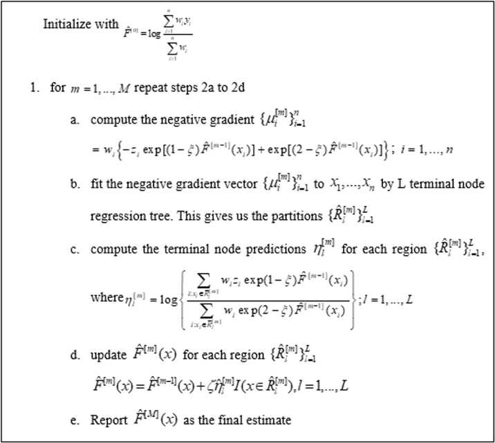
A forward stagewise algorithm is adopted to approximate the minimizer in Eq. (1), which then builds up the components of 𝛽^[m] h (x; 𝜉^m), (m = 1, 2, …, M) sequentially through a gradient descent-like procedure. At each iteration m (m = 1, 2, …), suppose the current estimate for $\bar{F}(\cdot )$ is $\hat{F}^{[m-1]}(\cdot )$ , we want to update $\hat{F}^{[m-1]}(\cdot )$ to $\hat{F}^{[m]}(\cdot )$ along the negative gradient direction of R _n(F).

The negative gradient vector $({\mu}_{1}^{[m]},\ldots ,{\mu}_{n}^{[m]})$ of R _n(F) with respect to F at $[F(x_{i})=\hat{F}^{[m-1]}(x_{i})]_{i=1}^{n}$ , can be written as $\begin{eqnarray}\displaystyle {\mu}_{i}^{[m]}=-\displaystyle \frac{\partial R_{n}(F)}{\partial F(x_{i})}. & & \displaystyle\end{eqnarray}$ (3) Gradient boosting fits the negative gradient vector ${\mu}_{j}^{[m]}$ for j = i: n as the working response to (x ₁, …, x _n) as the predictor to find a base learner h (x; 𝜉^[m]). The fitted h (x; 𝜉^[m]) can be viewed as an approximation of the negative gradient and can be evaluated on the entire space of x. The expansion coefficient 𝛽^[m] can then be determined by a line search $\begin{eqnarray} \displaystyle \hspace{-16.0pt}{\beta}^{[m]} & = & \displaystyle \mathop{\text{argmin}}_{{\beta}}\nonumber\\ \displaystyle \text{} & \text{} & \displaystyle \times \left\{\mathop{\sum }_{i=1}^{n}{\varphi}(y_{i},\hat{F}^{[m-1]}(x_{i})+{\beta}h(x;{\xi}^{[m]}))\right\}. \nonumber\\ \end{eqnarray}$ (4) As a consequence the estimation of $\bar{F}(x)$ for the next stage is $\begin{eqnarray}\displaystyle \hat{F}^{[m]}(x):=\hat{F}^{[m-1]}(x)+{\nu}{\beta}^{[m]}h(x;{\xi}^{[m]}), & & \displaystyle\end{eqnarray}$ (5) where (0 < 𝜈 ≤ 1) is the shrinkage parameter that controls the updating size (Friedman [16], Yang et al. [36]). A small 𝜈 imposes more shrinkage while 𝜈 = 1 gives complete negative gradient steps. Friedman [15] also indicated that the shrinkage parameter reduces over-fitting and improves predictive accuracy. The principal consideration in using this approach is by identifying the appropriate loss function of the empirical data.

2.2. The Tweedie compound Poisson model

This section briefly introduces compound Poisson distribution and the Tweedie model as a basis for our model formulation and analysis. Let N be a Poisson random variable denoted by Pois (𝜆) and let Y denote independent and identically distributed gamma random variables denoted by Gamma (𝛼, 𝜔) with mean 𝛼𝜔 and variance 𝛼𝜔². Define a random variable Z by $\begin{eqnarray} \displaystyle\hspace{-16.0pt} Z=\left\{ \begin{array}{@{} ll@{}}0, & \text{if }N=0\\ Y_{1}+Y_{2}+\cdots +Y_{N}, & \text{if }N=1,2,\ldots \\ \end{array} \right\}. & & \displaystyle \end{eqnarray}$ (6) Thus Z is the Poisson sum of independent Gamma random variables. The resulting F _Z distribution is referred to as compound Poisson distribution [10,32], which closely relates with exponential dispersion models (EDM). Notice that the distribution of Z (F _Z) has a probability mass at zero (P (Z = 0) = exp(−𝜆)). Also Z is conditional on k is Gamma (k𝛼, 𝜔). This means that the distribution function of Z can be written as $\begin{eqnarray}\displaystyle f_{z}(z|{\lambda},{\alpha},{\omega}) & = & \displaystyle P(N=0)d_{0}(z)\nonumber\\ \displaystyle \text{} & \text{} & \displaystyle +∼\mathop{\sum }_{k=1}^{\infty }P(N=k)f_{Z|N=k}(z)\nonumber\\ \displaystyle & = & \displaystyle \exp (-{\lambda})d_{0}(z)\nonumber\\ \displaystyle \text{} & \text{} & \displaystyle +∼\mathop{\sum }_{k=1}^{\infty }{\displaystyle \frac{{\lambda}^{k}e^{-{\lambda}}z^{k{\alpha}-1}e^{z/{\omega}}}{j!{\omega}^{k{\alpha}}{\Gamma}(k{\alpha})}},\end{eqnarray}$ (7) where d ₀ is the Dirac delta function at zero and f _Z∣N=k(z) is the conditional density of Z given N = k. This gives the cumulant generating function of Z $\begin{eqnarray}\displaystyle \log M_{z}(t)={\lambda}(1-{\omega}t)^{-{\alpha}}-1. & & \displaystyle\end{eqnarray}$ (8) According to Smyth [31] the compound Poisson distribution belongs to a special Exponential Dispersion Models (EDM) called the Tweedie models. The distribution of EDMs can be expressed in the form $\begin{eqnarray}\displaystyle f_{Z}(z\mid {\theta},{\phi})=a(z,{\phi})\exp \left\{\frac{z{\theta}-{\kappa}({\theta})}{{\phi}}\right\}, & & \displaystyle\end{eqnarray}$ (9) where a (⋅) is a normalizing function, 𝜅(⋅) is called the cumulant function, and both a (⋅) and 𝜅(⋅) are known. The parameter 𝜃 is in Re and the dispersion parameter 𝜙 is in Re ⁺. The main property of of EDMs is that $E(Z)={\mu}=\dot{{\kappa}}({\theta})$ and the variance $\text{Var}(Z)={\phi}\ddot{{\kappa}}({\theta})$ , where $\dot{{\kappa}}({\theta})$ and $\ddot{{\kappa}}({\theta})$ are the first and second derivatives of 𝜅(𝜃) respectively. The cumulant function of EDMs is $\begin{eqnarray}\displaystyle \log M_{Z}(t)=\displaystyle \frac{1}{{\phi}}\{{\kappa}({\theta}+{\phi}t)-{\kappa}({\theta})\}, & & \displaystyle\end{eqnarray}$ (10) Tweedie models are special cases of the EDMs characterized by power mean-variance relationship such that Var (Z) = 𝜙𝜇^𝜉, where 𝜉 is an index parameter. This mean-variance relation gives $\begin{eqnarray}\displaystyle {\theta}=\left\{\begin{array}{@{}cc@{}}\displaystyle \frac{{\mu}^{1-{\xi}}}{1-{\xi}}, & {\xi}\neq 1\\[3.0pt] \log {\mu}, & {\xi}=1\end{array}\right\} & & \displaystyle \nonumber\end{eqnarray}$ and $\begin{eqnarray}\displaystyle {\kappa}({\theta})=\left\{\begin{array}{@{}cc@{}}\displaystyle \frac{{\mu}^{2-{\xi}}}{2-{\xi}}, & {\xi}\neq 2\\[3.0pt] \log {\mu}, & {\xi}=2\end{array}\right\}. & & \displaystyle \nonumber\end{eqnarray}$ It can be shown that the compound Poisson distribution belongs to the class of Tweedie models. Thus, if we replace the parameters (𝜆, 𝛼, 𝜔) in the cumulant function in Eq. (8) by $\begin{eqnarray}\displaystyle \begin{array}{@{}c@{}}\displaystyle {\lambda}=\frac{1}{{\phi}}\left(\frac{{\mu}^{2-{\xi}}}{2-{\xi}}\right),\quad {\alpha}=\left(\frac{2-{\xi}}{{\xi}-1}\right),\\[5.0pt] \displaystyle {\omega}={\phi}({\xi}-1){\mu}^{{\xi}-1}\end{array} & & \displaystyle\end{eqnarray}$ (11) the cumulant function of the compound Poisson model has the form of a Tweedie model. As a result we consider Eq. (6) as the Tweedie compound Poisson model denoted by Tw (𝜇, 𝜙, 𝜉), where 1 < 𝜉 < 2 and 𝜇 > 0. The log-likelihood of the Tweedie model is $\begin{eqnarray}\displaystyle \log f_{Z}(z|{\mu},{\phi},{\xi}) & = & \displaystyle \frac{1}{{\phi}}\left(z\frac{{\mu}^{1-{\xi}}}{1-{\xi}}-\frac{{\mu}^{2-{\xi}}}{2-{\xi}}\right)\nonumber\\ \displaystyle \text{} & \text{} & \displaystyle +∼\log a(z,{\phi},{\xi}),\end{eqnarray}$ (12) where the normalizing function a (⋅) can be written as $\begin{eqnarray}\displaystyle \text{} & \text{} & \displaystyle \hspace{-25.0pt}a(z,{\phi},{\xi})\nonumber\\ \displaystyle \text{} & \text{} & \displaystyle \hspace{-29.0pt}\quad =\left\{\begin{array}{@{}ll@{}}\displaystyle \frac{1}{z}\mathop{\sum }_{t=1}^{\infty }W_{t}(z,{\phi},{\xi})=\frac{1}{z}\mathop{\sum }_{t=1}^{\infty } & \\ \displaystyle \times ∼\frac{z^{t{\alpha}}}{({\xi}-1)^{t{\alpha}}{\phi}^{t(1+{\alpha})}(2-{\xi})^{t}t!{\Gamma}(t{\alpha})}, & \text{for }z>0\\[3.0pt] 1, & \text{for }z>0,\end{array}\right\}\nonumber\end{eqnarray}$ where 𝛼 = (2 −𝜉)∕(𝜉 −1). A significant desirable property of Tweedie models is that they are the only EDMs that are scale invariant (Jorgensen and de Souza [21]). This means that if Z is a Tweedie variable with mean 𝜇 and dispersion 𝜙, then 𝜌Z follows the same distribution with mean 𝜌𝜇 and dispersion 𝜌^2−𝜉𝜙. This property makes Tweedie distributions a good choice for modeling data with an arbitrary monetary unit.

Yang et al. [36] integrated the Tweedie model into the tree-based gradient boosting algorithm by Friedman to model insurance claim size.

2.3. Model description and assumptions

In Non-Life insurance, the risk premium represents the expected cost of all claims declared by policyholders during the insured period. The calculation of the premium is based on statistical models that seeks to incorporate all available information about the accepted risk, thereby aiming at a more accurate assessment of tariffs attributed to each. The basis for calculating the risk premium is the statistical modeling of frequency and cost of claims that depends on the characteristics defined in the insurance contract. The risk premium is the mathematical expectation of the annual cost of claims declared by policyholders and it is obtained by multiplying the two components; the estimated frequency E (N) and expected cost of claims E (Y ): the risk premium for the ith policyholder is $\begin{eqnarray}\displaystyle \mathop{\sum }_{j=1}^{N_{i}}Y_{j}=E(Y_{i})E(N_{i}). & & \displaystyle\end{eqnarray}$ (13) In the classical risk model, it is assumed that the claim arrival process is a Poisson process. This assumption implies a constant claim arrival intensity but in most practical cases, such assumption is inadequate. In such situations Cox process can be used as an alternative. Cox process is a doubly stochastic Poisson process which has stochastic claim arrival intensity rate. A general treatment of Cox process is presented in Rolski et al. [30]. The study considers a process (Markov-modulated), where the claim intensity is assumed to be homogeneous within each state but heterogeneous among states. A brief pictorial description is shown in Fig. 1 where, $Y^{(i)}=\sum _{j=1}^{n}Y_{j}^{(i)}$ , is the total claim size in state 𝛶⁽ⁱ⁾, $Y_{j}^{(i)}$ is a non-negative random variable that represents jth claim in state i for i = (1, …, k), j = (1, …, n) and N ⁽ⁱ⁾(t) represents the number of claims in state 𝛶⁽ⁱ⁾ at time t. In the Markov-modulated Poisson process, the claim number process is defined as N = N (t), t > 0 as a function of a Markov chain M = M (t), t > 0, with finite state space $\{{\Upsilon}^{(1)},\ldots ,{\Upsilon}^{(k)}\}$ .

Fig. 1.

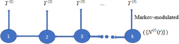
The conceptual framework of the study.

The study assumes that risk of accident varies from one state to another and from time to time. Factors such as vehicle density, road network, traffic regulation etc. may vary from one state to another and hence risk propensity may vary likewise. More specifically, suppose Y _j is a non-negative random variable corresponding to the amount of the jth claim. Also let assume that the random variables Y _j are equally defined as a function of the Markovian process M. This means that beside historical risk, claim arrival process at time t depends on the behaviour of the process M at time t. The behavior of this process is captured as location risk of a policy.

2.4. Model specification

The study consider a portfolio of policies of the form $\{(y_{i},X_{i},w_{i},{\gamma}_{j})\}$ for n independent insurance contracts, where for the ith contract, y _i is the policy’s claim amount, X _i is the historical risk, w _i is the duration of the policy and 𝛾_j is the Markovian risk factor that characterizes the risk specific to the geographical location.The location and historical risk are vector of explanatory variables that characterize the policyholder and the risk being insured. We propose that the expected risk premium for a policy is determined by a predictor function. $\begin{eqnarray}\displaystyle E(Z)=f(H,L), & & \displaystyle\end{eqnarray}$ (14) where H is the historical risk and L is the geographical location risk. We thus define the expected risk premium for policy i in location j as $\begin{eqnarray}\displaystyle {\eta}({\mu}_{ij})={\vartheta}_{ij}\ell _{ij}+{\alpha}_{ij}\hbar_{ij}, & & \displaystyle\end{eqnarray}$ (15) where 𝜗_ij is the associated risk factor for each policy in location j, 𝛼_ij are the historical risk factors associated with each policy and 𝜂 is the link function that relates the expected premium to the risk factors in Eq. (15). Historical risk is defined as the risk specific to the policy characteristics, while location risk is specific to the geographical location in which the policy usually operates. We derive the risk for each state via accident matrix obtained via Markov chain of which we briefly explain.

Given that the occurrence of an accident at time t is a stochastic sequence, we characterize and discretize our risk model into ten (10) states based on the ten geographical states in Ghana (j = 1,2, …,10). Given the initial probabilities x ₀ of the event E in state j at period t. We compute the transition matrix M for period t via Bayes theorem. Let P (E) denote the long run proportion of times the event E occurs upon repeated sampling during time t. In otherwords how likely it is that a vehicle operating within state j or between states will experience event E. Furthermore denote P (E _t1) the risk of occurence of an accident in state one at time t and P (E _t2) the occurence of an event at time t in state two etc. In the context of our study and mathematical tractability, we define E _t1 E _t2 as the event that a vehicle operates between two states. This means that P (E _t1 E _t2) represent the risk involved when operating between two states. Given that E _t1 and E _t2 are independent, P (E _t1 E _t2) = P (E _t1)P (E _t2). Thus the probability distribution of accident risk can be expressed as a transition matrix as $\begin{eqnarray}\displaystyle M=\left[\begin{array}{@{}cccccc@{}}m_{11} & m_{12} & . & . & . & m_{1k}\\[3.0pt] m_{21} & m_{22} & . & . & . & m_{2k}\\[3.0pt] \vdots & \vdots & \vdots & \vdots & \vdots & \vdots \\[3.0pt] m_{k1} & m_{k2} & . & . & . & m_{kk}\end{array}\right], & & \displaystyle\end{eqnarray}$ (16) where _ij represents accident risk from state i to state j and _kk represent accident risk within state k, which could be written in the form of a transition matrix M, such that the sum of each row of M equals 1 If a discrete time Markov chain $\{M\}$ is irreducible and aperiodic then it has a limiting and stationary distribution. Thus, $\begin{eqnarray}\displaystyle \mathop{\lim }_{n\rightarrow \infty }M^{n}={\gamma}_{j}. & & \displaystyle \nonumber\end{eqnarray}$ Thus, the limiting distribution is derived such that $\begin{eqnarray}\displaystyle {\gamma}_{j}={\gamma}_{j}M, & & \displaystyle\end{eqnarray}$ (17) where 𝛾_j is the stationary distribution of accident risk for state 𝛶⁽ⁱ⁾; (i = 1, …, k) The outcome in Eq. (17) is used as a basis to classify the geographical location risk into three risk zones namely: considerable, medium and minimal risk zones represented by 𝜗 in Eq. (15). The classification therefore depends on the behaviour of the process observed in M from time to time and hence the risk classification is Markov-driven.

2.5. Materials

We obtained data from two sources; An auto-insurance data was obtained from a major insurance company in Ghana. The data spans from 2013 to 2016. The data contains claim history and other characteristics of policyholders. In line with the study objectives, an auxiliary data was obtained from National Road Safety Commission on the number of road traffic accidents that spans from 2001 to 2015. The National Road Safety Commission is a state agency responsible for safety education and accident statistics in Ghana. The data include road traffic information for all the ten geographical regions of Ghana.

3. Analysis and results

The paper considers two sets of data an accident data and insurance data as described in Section 2.5.

3.1. Summary of accident data

We use the crash data to derive the location risk. The probability distribution of the accident risk, the transition matrix and the stationary distribution is shown in Table 1, Table 2 and Table 3, respectively. Table 1 is the probability distribution of accident risk accross the ten regions of Ghana as per the data, Table 2 represents the transition matrix derived from Section 2.4 and Table 3 derived from Eq. (17).

Table 1
Accident matix for the ten geographical zones

GR AS ER CR WR BA VR NR UW UE Total

GR 0.4240 0.0657 0.0445 0.0377 0.0259 0.0250 0.0208 0.0123 0.0064 0.0059 0.6682

AS 0.0657 0.1550 0.0163 0.0138 0.0095 0.0091 0.0076 0.0045 0.0023 0.0022 0.2860

ER 0.0445 0.0163 0.1050 0.0093 0.0064 0.0062 0.0051 0.0030 0.0016 0.0015 0.1990

CR 0.0377 0.0318 0.0093 0.0890 0.0054 0.0053 0.0044 0.0026 0.0013 0.0012 0.1701

WR 0.0259 0.0095 0.0064 0.0054 0.0610 0.0036 0.0030 0.0018 0.0009 0.0009 0.1183

BA 0.0250 0.0091 0.0062 0.0053 0.0036 0.0590 0.0029 0.0017 0.0009 0.0008 0.1145

VR 0.0208 0.0076 0.0051 0.0044 0.0030 0.0029 0.0490 0.0014 0.0007 0.0007 0.0956

NR 0.0123 0.0045 0.0030 0.0026 0.0018 0.0017 0.0014 0.0290 0.0004 0.0004 0.0572

UW 0.0064 0.0023 0.0016 0.0013 0.0009 0.0009 0.0007 0.0004 0.0150 0.0002 0.0298

UE 0.0059 0.0022 0.0015 0.0012 0.0009 0.0008 0.0007 0.0004 0.0002 0.0140 0.0278

	GR	AS	ER	CR	WR	BA	VR	NR	UW	UE	Total
GR	0.4240	0.0657	0.0445	0.0377	0.0259	0.0250	0.0208	0.0123	0.0064	0.0059	0.6682
AS	0.0657	0.1550	0.0163	0.0138	0.0095	0.0091	0.0076	0.0045	0.0023	0.0022	0.2860
ER	0.0445	0.0163	0.1050	0.0093	0.0064	0.0062	0.0051	0.0030	0.0016	0.0015	0.1990
CR	0.0377	0.0318	0.0093	0.0890	0.0054	0.0053	0.0044	0.0026	0.0013	0.0012	0.1701
WR	0.0259	0.0095	0.0064	0.0054	0.0610	0.0036	0.0030	0.0018	0.0009	0.0009	0.1183
BA	0.0250	0.0091	0.0062	0.0053	0.0036	0.0590	0.0029	0.0017	0.0009	0.0008	0.1145
VR	0.0208	0.0076	0.0051	0.0044	0.0030	0.0029	0.0490	0.0014	0.0007	0.0007	0.0956
NR	0.0123	0.0045	0.0030	0.0026	0.0018	0.0017	0.0014	0.0290	0.0004	0.0004	0.0572
UW	0.0064	0.0023	0.0016	0.0013	0.0009	0.0009	0.0007	0.0004	0.0150	0.0002	0.0298
UE	0.0059	0.0022	0.0015	0.0012	0.0009	0.0008	0.0007	0.0004	0.0002	0.0140	0.0278

Source: Authors computation (2018).

Table 2

A 10-dimensional discrete time Markov chain defined by the ten

	GR	AS	BA	CR	ER	NR	UE	UW	VR	WR
GR	0.5566	0.1119	0.0532	0.0585	0.0822	0.0240	0.0170	0.0106	0.0389	0.0472
AS	0.1131	0.5559	0.0531	0.0584	0.0820	0.0240	0.0169	0.0106	0.0389	0.0471
BA	0.1068	0.1056	0.5251	0.0552	0.0775	0.0227	0.0160	0.0100	0.0367	0.0445
CR	0.1074	0.1061	0.0504	0.5277	0.0779	0.0228	0.0161	0.0100	0.0369	0.0448
ER	0.1098	0.1085	0.0516	0.0567	0.5398	0.0233	0.0165	0.0102	0.0377	0.0458
NR	0.1040	0.1027	0.0488	0.0537	0.0754	0.5110	0.0156	0.0997	0.0357	0.0433
UE	0.1033	0.1021	0.0485	0.0533	0.0749	0.0219	0.5077	0.0096	0.0355	0.0431
UW	0.1027	0.1015	0.0482	0.0530	0.0745	0.0218	0.0154	0.5048	0.0353	0.0428
VR	0.1054	0.1042	0.0495	0.0544	0.0765	0.0224	0.0158	0.0098	0.5181	0.0439
WR	0.1062	0.1050	0.0499	0.0548	0.0771	0.0159	0.0099	0.0365	0.3651	0.5221

Table 3

Long run distribution of accident risk

GR	AS	BA	CR	ER	NR	UE	UW	VR	WR
0.1964	0.1943	0.0978	0.1069	0.1469	0.0453	0.0323	0.0202	0.0725	0.0873

Fig. 2.

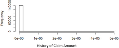
Distribution of claims (2013–2016).

Fig. 3.

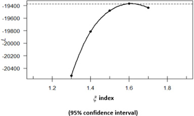
Estimating the optimal index parameter (𝜉).

Fig. 4.

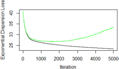
A plot of CV error showing the optimal iteration number.

Thus, Table 3 shows the long run distribution of accidents risk across the ten regions of Ghana. This means that in the long run accidents risk within Greater Accra region is about 19.64%, Ashanti 19.43%, Brong Ahafo 9.78%, Central region 10.69%, Eastern region 14.69%, Northern region 4.53%, Upper East region 3.23%, Upper West 2.02%, Volta region 7.25% and Western region is 8.73%. For mathematical tractability the study sought to reclassify the ten states into three based on risk similarities consistent with Occams razor. The result of the classification is described: Thus Greater Accra and Ashanti regions were classified as considerable risk zone, Brong Ahafo, Central region, Eastern region, Western region and Volta region classified as medium risk zones, while Northern region, Upper west and Upper east were classified as low risk zone. This classification is Markov-driven over a period of time, depending on the behaviour or the changing dynamics of the risk matrix in Table 1.

3.2. Summary of insurance data

The insurance data consists of policy and claim information for each vehicle. The data contains one hundred and forty thousand, nine hundred and sixty-one (140,961) vehicle records out of which contains five thousand, four hundred and fifty (5450) claims records for four (4) years, from 2013 to 2016. Table 4 summarizes the variables of the data set.

Table 4
Insurance policy variables

Policy characteristics Vehicle characteristics Claim history

Use type Vehicle make Number of claims

1. Commercial 1. Opel

2. Private 2. Nissan

3. Mitsubishi

Usage category: 4. Kia

1) Taxis, 5. Tata

2) Ambulance, 6. Toyota

3) Tanker, 7. BMW

4) General cartage, 8. Hyundai

5) Maxi-bus, 9. Daewoo

6) Mini-bus, 10. Honda

7) Private individual, 11. Audi

8) Corporate individual, 12. Peugeot

9) Motor, 13. Ford

10) Own goods carrying, 14. Daf

11) Hiring, 15. Mercedes

12) Special types 16. Mazda

17. Make.Other

Policy coverage Vehicle age Region Claim amount

1. Comprehensive

2. Third Party

3. Third PartyFire and Theft

Policy characteristics	Vehicle characteristics	Claim history
Use type	Vehicle make	Number of claims
1. Commercial	1. Opel
2. Private	2. Nissan
	3. Mitsubishi
Usage category:	4. Kia
1) Taxis,	5. Tata
2) Ambulance,	6. Toyota
3) Tanker,	7. BMW
4) General cartage,	8. Hyundai
5) Maxi-bus,	9. Daewoo
6) Mini-bus,	10. Honda
7) Private individual,	11. Audi
8) Corporate individual,	12. Peugeot
9) Motor,	13. Ford
10) Own goods carrying,	14. Daf
11) Hiring,	15. Mercedes
12) Special types	16. Mazda
	17. Make.Other
Policy coverage	Vehicle age Region	Claim amount
1. Comprehensive
2. Third Party
3. Third PartyFire and Theft

Fig. 5.

A schematic overview of the TD boost model.

Figure 2 also shows the distribution of total claim amount recorded from 2013 to 2016. The figure suggests high skewness. This is expected as claims rarely occurs and when it occurs, the severity of it when it occurs has been the bane of the non-life insurance industry.

Fig. 6.

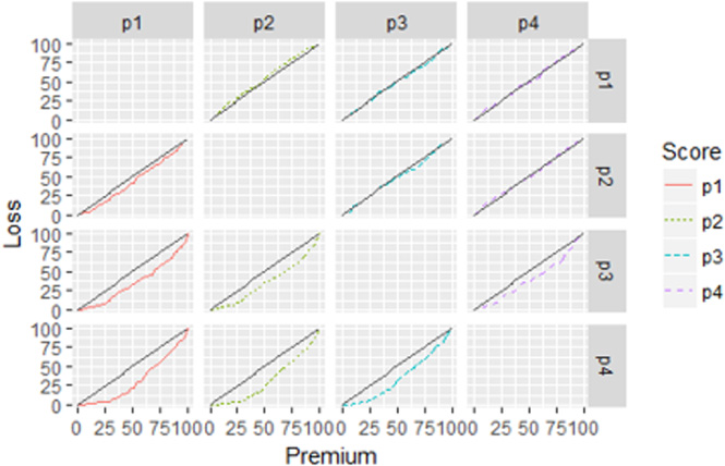
Plot of ordered Lorenz curve.

From Table 5, there were approximately 140,961 insured customers of which about 5450 (3.9%) filed for claims. About 85% of the claims in the study period occurred in Greater Accra region and the lowest claims frequency resulting occurred in Upper West region. The total claim size recorded for the study period was Ghana cedis (GHS) 43,364,372 while the premium income accrued from claimants is GHS 7,630,261 representing about 17.6% of aggregate claims. This means that less than a quarter of claims was accounted for by the premium income for the period. In terms of regional distribution of total claims, Greater Accra region recorded the highest of the aggregate claims (85%) but contributed about 83% of the premium income. Ashanti region recorded the second highest (about 8%), while Upper West recorded the lowest (0.09%). These are not surprising since nearly 75.4% of the total insured are in the Greater Accra region, and less than 0.3% of same are in the upper west region. In terms third party and comprehensive segregation, the data showed that a claim of approximately GHS 5,284,407 was recorded for third party representing 12.06% of total claims and approximately GHS 38,516,284 for comprehensive representing 87.94% of total claims. No claims were recorded for third party fire and theft. This means that majority (about 88%) of total claims was made on comprehensive policies.

Table 5

Regional distribution of claims (2013–2016)

Region of incidence	No. of Claim	No. of Vehs. Insured	No. of Claims/No. of Veh. Insured	Claim proportion	Claim size (Ghs)	Premium Income (Ghs)
Ashanti	512	21143	0.0242	0.0796	3,453,901	547,326
Brong Ahafo	55	1962	0.0280	0.0059	254,983	79,426
Central	60	1731	0.0347	0.0074	322,927	75,762
Eastern	154	3291	0.0393	0.0298	1,293,609	214,743
Greater Accra	4407	106232	0.0415	0.8532	36,997,062	6,337,100
Northern	27	759	0.0356	0.0029	127,307	37,581
Upper East	24	696	0.0345	0.0027	116,862	36,828
Upper West	4	416	0.0096	0.0009	37,883	7,558
Western	149	3148	0.0473	0.0104	451,503	201,352
Volta	58	953	0.0609	0.0071	308,335	92,581
Total	5450	140961	0.03866	1.0000	43,364,372	7,630,261

3.3. Estimating the risk premium function

As discussed in Section 2, the study considered the distribution of accident risk across the ten regions of Ghana. To the best of our knowledge no such information has been considered in insurance pricing in the both developing and the developed economies. The author reckon that several factors influence insurance outcomes. Some of the factors include regulation and legislative changes, claim trends, vehicle density, interest rate and investment. Legislative and regulation, inflation, interest rate and investment could be regarded as fixed. However, claim trends, vehicle congestion and for that matter accidents risk in different geographical zones could vary from one region to the other as well as from time to time. More so, factors such as, roadway design, roadway maintenance have been shown to contribute significantly to road accidents which vary from one region to another. For this reason, these phenomena are characterized and incorporated into the pricing framework. The study used Markov theory to categorize the claims data set based on accident risk derived for each region.

Two indicator variables ℓ ₁ and ℓ ₂ were adopted to integrate the three levels of geographical location risk into the risk premium prediction function in Eq. (15). In Table 4, the claim amount and claim frequency represent the outcome variables. The rest of the variables represent and were considered as the historical risk factors for non-life insurance claims.

The study estimates the predictor function of the model using the method discussed in Section 2. Consistent with statistical model framework, 70% of the data was randomly selected to be used in building the model, while 30% is used for out-of-sample validation of the model. As discussed in Sections 2.1 and 2.2, the first choice in building a Tweedie gradient boosting model involves selection of the appropriate loss function which we specify as Tweedie. With Tweedie loss function, the method requires specification of the index parameter (𝜉;1 < 𝜉 < 2), the shrinkage (𝜁;0 < 𝜁 < 1), the optimal number of trees and the interaction depth (L).

The optimal index parameter was obtained using profile likelihood estimation method Yang et al. [36]. As shown in Fig. 3, the optimal 𝜉 obtained was 1.61 at 5% level of significance.

We also adopt a selection procedure to obtain the optimal M. To illustrate the selection procedure, we first grew many trees with M = 5000 and plot the error rate associated each tree size. This is done using a five-fold cross validation.This means that the data was randomly divided into five (5) samples not necessary equal size. Each of the five (5) sample is fitted separately to the model. Out of which the optimal number of trees is obtained. As shown in Fig. 4 the curve colored green represents the error rate at various levels of iterations. As the tree grows from point zero (0) onwards the error rate reduces suggesting an improvement of error reduction rate. As the model moves beyond 2000 iterations, the curve turn upwards suggest diminishing returns of model accuracy. The point where the improvement in error rate reaches its maximum is the optimal tree number which from Fig. 4 is given as M = 1788. We further examined the optimal interaction size (L). It is worth noting that a model with a one-way interaction effects is simply an additive model. The study evaluated 20, 10, 5, 4, 3 and 2 way interaction effects using the training data set. The result showed that the ten (10) way interaction effects gives relatively better results (L = 10). Our shrinkage parameter was also set at 0.05 (Friedman [15]). Based on the specifications; M = 1788, shrinkage parameter (𝜍 = 0.05) and 𝜉 = 1.67, we estimate the predictor function in Eq. (12) considering (15) and using the procedure described in Section 2.1. A schematic overview of the algorithm by Yang et al. [36] is shown in Fig. 5. The resulting model summary is shown in Appendix Tables 6 and 7.

Tables 6 and 7 present the variables considered with their relative importance. In an attempt to assess how important each variable is to the model as in regression trees we calculate the total amount of reduction in the Residual Sum of Squares (RSS) attributable to splits caused by the predictor and averaged over the number of trees. In classification trees, we do the same thing using average reduction in the Gini index. The location effect as specified by the model Eq. (15) was significant. Thus, while state 1 contribute about 0.08%, state 2, contribute about 0.6%. This is significant considering the nature of business of the non-life insurance business and the severity of claims when it occurs.

3.4. Model evaluation

The study compares the Markov-modulated Gradient Boosting model which has integrated location risk with other conventional models. We considered a TDboost without location risk, (TDBOOST), Tweedie Generalized Linear Model (TGLM), Gradient boosting approach by Guelman [17]. To examine the performance of these competing models, after fitting each on the training data, we predict the risk premium $Z(X)=\hat{{\mu}}(X)$ by applying each model on the independent out-of-sample data. Due to the data structure it would not be appropriate to measure differences between predicted premiums Z (X) and the real loss y by depending on mean square error loss or the mean absolute loss. This is because the losses or claims has high proportion of zeros and very much positively skewed. An alternative statistical measure was considered. The Ordered Lorenz curve and the associated Gini index proposed by Frees et al. [11] was considered. This measure captures the discrepancy between premium and loss distributions without the influence of the zeros nor skewness. we compute the gini index and calculate the ratio of the rate we would charge based on MMGB model to the rate we would charge based on GLM, TDboost and GBM.

Mathematically, suppose B (X) is the base premium, we define the relative premium as $\begin{eqnarray}\displaystyle R(X)=\frac{Z(X)}{B(X)}. & & \displaystyle\end{eqnarray}$ (18)

A low relativity is interpreted as the policy that is highly profitable and a suitable candidate to retain. This means that if the score Z (X) is the desirable approximation of the expected loss. Then, if the relativity is small, then we expect a small loss relative to the premium. If the relativity is large we expect a large loss relative to the premium (Werner and Modlin [33], Frees et al. [12]). In addition, under relativity ordering a large covariance between losses and the proportion of premiums retained implies a high Gini index. A large negative covariance between premiums and relativities implies a high Gini index. The ordered premium and loss distribution is given respectively as $\begin{eqnarray} \displaystyle \hat{D}_{P}(S)=\displaystyle \frac{\displaystyle\sum_{i=1}^{n}B(x_{i})I(R(x_{i})\leq s)}{\displaystyle\sum_{i=1}^{n}B(x_{i})} & & \displaystyle \end{eqnarray}$ (19) and $\begin{eqnarray} \displaystyle \hat{D}_{L}(S)=\frac{\displaystyle\sum_{i=1}^{n}y_{i}(I(R(x_{i})\leq s))}{\displaystyle\sum_{i=1}^{n}y_{i}}. & & \displaystyle \end{eqnarray}$ (20)

The two distributions (19) and (20) are based on the same sorting criteria. The Ordered Lorenz curve is the graph of $(\hat{D}_{L}(S),\hat{D}_{L}(S)).$ When the proportion of losses equals the proportion of premiums for the insurer, the curve equals the 45-degree line (line of equality). Twice the area between the Ordered Lorenz curve and the line of equality measures the discrepancy between the premium and loss distributions, define as the Gini index. This means that a larger Gini index would imply a favorable model.

From (18) the prediction for R (X) from each model is successively specified as the base premium and use the predictions from the remaining models as the competing premium to compute the Gini indices. Using minimax strategy to select the best performing model, the study selected the model that provides the smallest of the maximal indices over the competing models.

Table 8 presents the Gini indices with their standard errors in Table 9. We find that the maximal Gini index is 1.38 when using MMGB as the base premium, 12.07, when using TDboost as base premium, 28.406 is when using GLM as base premium and 36.296 when using GBM as the base. MMGB is the smallest. Therefore, MMGB has the smallest maximum Gini index of 1.380, hence it is the least vulnerable to alternative scores.

3.5. Discussion of results

Several statistical techniques have been proposed to price premiums such as modelling the frequency and severity of claims and computing the product of its expectations (Haberman and Renshaw [19], Mihaela [27] etc.). There is constantly the need to improve on ways in which policy premiums are priced. In many actuarial risk models, consideration is mostly placed on internal historical claims data that are obtained within the insurance firm or industry. Thus, external data is rarely used. With unobservable phenomenon, researchers usually employ hidden Markov chains to make extrapolations (Guillou et al. [18], McNeil and Lindskog [26]). However, it is important to note that besides historical claims data in Auto insurance external observable phenomenon such as policy operational risk as a factor contribute significantly to loss cost. Practical tools for studying such phenomenon in a more flexible way has been a challenge. Results from our gini index suggested that the MMGB model defined risk relatively better the cases where such risk considerations are discounted. for some predictors could pose a challenge. More so as oppose to other non-linear statistical learning methods such as neural networks and support vector machines, Gradient boosting provides interpretable results via the relative influence of the input variables and their partial dependence plots (Guelman [17]). By considering location risk of a policy, the flexible Markov Modulated Tree-Based Gradient Boosting method which is designed to integrate location risk factor into insurance pricing framework was to be more efficient. Based on the sample data used in this analysis, the level of accuracy in predictions was shown to be higher for MMGB relative to other models. This is not surprising since GLMs are relatively simple linear models and are thus constrained by the class of functions they can approximate. In short, Markov-modulated gradient boosting framework is a viable alternative method for building insurance loss cost models such as Guelman [17], Yang et al. [36], Friedman [15,16] within the statistical learning framework.

4. Conclusion

We have presented a probabilistic Markov-modulated tree-based Gradient Boosting (MMGB) model that considers location risk in pricing auto-insurance premiums. We have shown that by integration of location risk or introducing geographical location risk as covariates, the insurance policies are better differentiated in terms of risk and priced efficiently. This could assist non-life insurance companies in underwriting and claims management for sustainability. We have shown that the MMGB model performs relatively better than, the cases where location risk is not considered.

4.1. Recommendations

In view of the above conclusions, to ensure sustainability and fairness in pricing, a model-based MMGB approach is recommended for risk premium pricing in Ghana and other sub-saharran countries where accident risk is diverse across geographical locations. This is because the model is flexible and fairly captures the distribution of the data structure and account for location risk for any given policy.

It is also recommended based on the findings that; the non-life insurance companies use the risk-based model as an additional tool to ascertain the level of risk for its clients.

Footnotes

Summary of model variables with their relative importance

Table 9

Matrix of standard errors

	MMGB(P1)	TDBOOST(P2)	GLM(P3)	GBM(P4)
MMGB	0.000	3.062	3.555	3.107
TDBOOST	3.045	0.000	3.570	3.140
GLM	3.246	3.266	0.000	3.412
GBM	2.273	2.304	2.869	0.000

References

Antonio

and Valdez

E.A.

, Statistical concepts of a priori and a posterior risk classification in insurance, Advances in Statistical Analysis 96(2) (2012), 187–224.

Anstey

K.J.

Wood

Lord

and Walker

J.G.

, Cognitive, sensory and physically factors enabling driving safety in older adults, Clinical Psychology Review 25 (2005), 45–65.

Breiman

, Arcing classifier (with discussion and a rejoinder by the author), The Annals of Statistics 26 (1998), 801–849.

Cossette

Landriault

and Marceau

, Compound binomial risk model in a Markovian environment, Insurance: Mathematics and Economics 35 (2004), 425–443.

Cramer

, Collective risk theory: A survey of the theory from the point of view of the theory of stochastic process, in: 7th Jubilee Volume of Skandia Insurance Company, Stockholm, 1955, pp. 5–92.

Denuit

and Lang

, Nonlife ratemaking with Bayesian GAMS, Mathematics and Economics 35(3) (2004), 627–717.

Dionne

Gourieroux

and Vanasse

, Testing for evidence of adverse selection in the automobile insurance market: A comment, Journal of Political Economy 109 (2001), 444–453.

Djuric

, Collective risk model in non-life insurance, Economic Horizon 15(2) (2013), 167–175.

Dunn

P.K.

and Smyth

G.K.

, Evaluation of Tweedie exponential dispersion model densities by Fourier inversion, Statistics and Computing 18 (2008), 73–86.

10.

Feller

, An Introduction to Probability Theory and its Applications, Wiley & Sons, New York, 1968.

11.

Frees

E.W.

Meyers

and Cummings

A.D

, Summarizing insurance scores using a Gini index., Journal of the American Statistical Association 106 (2011), 1085–1098.

12.

Frees

E.W.

Meyers

and Cummings

A.D.

, Predictive modelling of multi-peril homeowners insurance,, Variance (2012).

13.

Frees

E.W.

Meyers

and Cummings

A.D.

, Insurance ratemaking and a Gini index, Journal of Risk and Insurance (2013).

14.

Freund

and Schapire

R.E.

, A decision-theoretic generalization of on-line learning and an application to boosting, Journal of Computer and System Sciences 55(1) (1997), 119–139.

15.

Friedman

J.H.

, Greedy function approximation: A gradient boosting machine, Annals of Statistics 29(5) (2001), 1189–1232.

16.

Friedman

J.H.

, Stochastic gradient boosting, Computational Statistics and Data Analysis 38(4) (2002), 367–378.

17.

Guelman

, Gradient boosting trees for auto insurance loss cost modelling and prediction, Expert Systems with Applications 39 (2012), 3659–3667.

18.

Guillou

Loisel

and Stupfler

, Estimation of the parameters of a Markov-modulated process in insurance, Insurance: Mathematics and Economics (2013).

19.

Haberman

and Renshaw

A.E.

, Generalized linear models and actuarial science, Statistician 45 (1996), 407–436.

20.

Hastie

Friedman

and Tibshirani

, The Elements of Statistical Learning: Data Mining, Inference and Prediction, Second ed. Springer Series in Statistics, Springer, 2009.

21.

Jorgensen

and de Souza

M.C.

, Fitting Tweedies compound Poisson model to insurance claim data, Scandinavian Actuarial Journal (1994), 69–93.

22.

Kaas

Goovaerts

M.J.

Dhaene

and Denuit

, Modern Actuarial Risk Theory, Kluwer, Dordrecht, 2001.

23.

Loisel

, Ruin theory with K lines of business, in: Proceedings of the 3rd Actuarial and Financial Day, Brussels, 2004.

24.

McCullagh

and Nelder

J.A.

, Generalized Linear Models, Chapman and Hall, London, 1989.

25.

McCartt

A.T.

Shabanova

V.I.

and Leaf

W.A.

, Driving experience, crashes and traffic citations of teenage beginning drivers, Accident Analysis & Prevention 35 (2003), 311–320.

26.

McNeil

A.J.

and Lindskog

, Common Poisson shock models: Applications to insurance and credit risk modelling, in: Federal institute of Technology 2001.

27.

Mihaela

, Insurance pricing using generalized linear models, Procedia Economics and Finance 20 (2015), 147–156.

28.

Nelder

and Wedderburn

, Generalized linear models, Journal of Statistical Society Series A 135 (1972), 370–384.

29.

Ohlsson

and Johansson

, Non-life Insurance Pricing with Generalized Models, Springer, 2010.

30.

Rolski

Schmidli

Schmidt

and Teugels

, Stochastic Processes for Insurance and Finance, Wiley, New York, 1999.

31.

Smyth

G.K.

, Regression analysis of quantity data with exact zeros, in: Proceedings of the Second Australia-Japan Workshop on Stochastic Models in Engineering, Technology and Management, Citeseer 1996, pp. 572–580.

32.

Smyth

G.K.

and Jorgensen

, Fitting Tweedie’s compound Poisson model to insurance claims data: Dispersion modeling, ASTIN Bulletin 32 (2002), 143–157.

33.

Werner

and Modlin

, Basic Ratemaking, Fifth ed. Casualty Actuarial Society, 2010.

34.

Werner

Modlin

and Watson

W.T.

, Basic Ratemaking, Fifth ed. Casualty Actuarial Society, 2016.

35.

Wood

S.N.

, Generalized Additive Models: An Introduction, R. Chapman & Hall/CRC, 2006.

36.

Yang

Qian

and Zou

, Insurance premium prediction via gradient tree-boosted tweedie compound Poisson models, Journal of Business and Economic Statistics (2016).