
Abstract
The aim of this paper is to provide simple models with a time-varying Hurst index. Such models should be simple as much as possible and well fit the estimated Hurst index. After a recall on the fractional and multifractional Brownian motion and on the statistical estimation of the Hurst index, we propose a fitting test for a model with a time-varying Hurst index. Then, we give an approach to select a simple model. Our approach is illustrated by numerous numerical simulations and then applied to market finance data.
Keywords
Introduction
As the data become larger, the stochastic models to describe datasets become more and more elaborated. This paper concerns large or big time series, modeled by multifractional Brownian motion (mBm), mainly with applications to financial series. However, our results can be applied to other practical fields. Recall that mBm are fractional Brownian motion (fBm) where the constant Hurst index has been replaced by a time-varying Hurst index. Our claim is that mBm with a Hurst index being itself a stochastic process is an useless generalization. Statistics, more precisely sampling fluctuation, explain that, even for infinitely differentiable Hurst index, the usual time-varying Hurst index estimators are stochastic processes. Moreover, smooth enough time-varying Hurst index is relevant for many applications, whereas the more general model looks like a theoretical challenge for smart probabilist. So, we advocate more simple models with infinitely differentiable or piecewise smooth Hurst index.
The rest of this article is organized as follows. In Section 2, we give recalls on the fractional Brownian motion and multifractional Brownian motion. Then we give some statistics for fBm and mBm. After that, we explain the fitting test for a time-varying Hurst index in Section 3. In Section 4, we estimate the Hurst index for fBm and mBm and we give some results of numerical simulations using a software improved based on the one of [7]. Finally, in Section 5, we apply our approach on two real financial datasets.
Fractional and multifractional Brownian motion
The Brownian motion was introduced by Bachelier (1901) for stock options in finance and next by Einstein (1905) in order to describe successive movements of atomic particles independent one from another. The mathematical theory was developed by Wiener during the 1920’s. In 1940, Kolmogorov has introduced the fractional Brownian motion, which was popularized by Mandelbrot since the 1960’s [35], the precise definition is postponed in Section 2.1. At these times (during 1970’s and 1980’s), we only have access to small time series. For example, the CAC 40 (Cotation Assistée en Continu = Electronic Continuous time trading) was adopted at Paris Bourse in 1987. Similar technological progresses arise in other practical fields. Time series observed at higher frequencies point that Hurst index is not constant but often vary over time. The multifractional Brownian motion was then introduced in [10,39]. The mBm is a fBm where the Hurst index H becomes a time-varying function
Recall on fractional Brownian motion
In this paper, we aim to give a method for selecting a good probabilistic model with a time-varying Hurst index. To begin, we give an overview of the process we are working with. The multifractional Brownian motion (mBm) can be viewed as a generalisation of the fractional Brownian motion (fBm), which is defined as follows:
The fBm
The fBm has stationary increments, it admits different representations, see e.g. [12], and can be also viewed as a Gaussian field depending both on the time t and the Hurst index H. For instance, the harmonisable representation of the fBm considered as a Gaussian field is given by
The mBm is a generalisation of the fBm where the Hurst index H is replaced by a time-varying function
Let
Due to the time-varying Hurst index, stationarity of the increments does not hold anymore, therefore long range dependency becomes a meaningless notion. Similarly, global self-similarity no more holds, but mBm verifies local asymptotic self-similarity of order
Figures 1 and 2 below show a path of a multifractional Brownian motion with two Hurst index functions. The software used is based on a code of [6] that we have improved for our study.
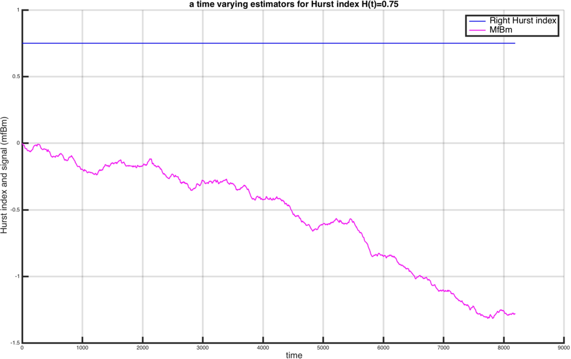
A path of mBm with Hurst index

A path of mBm with Hurst index
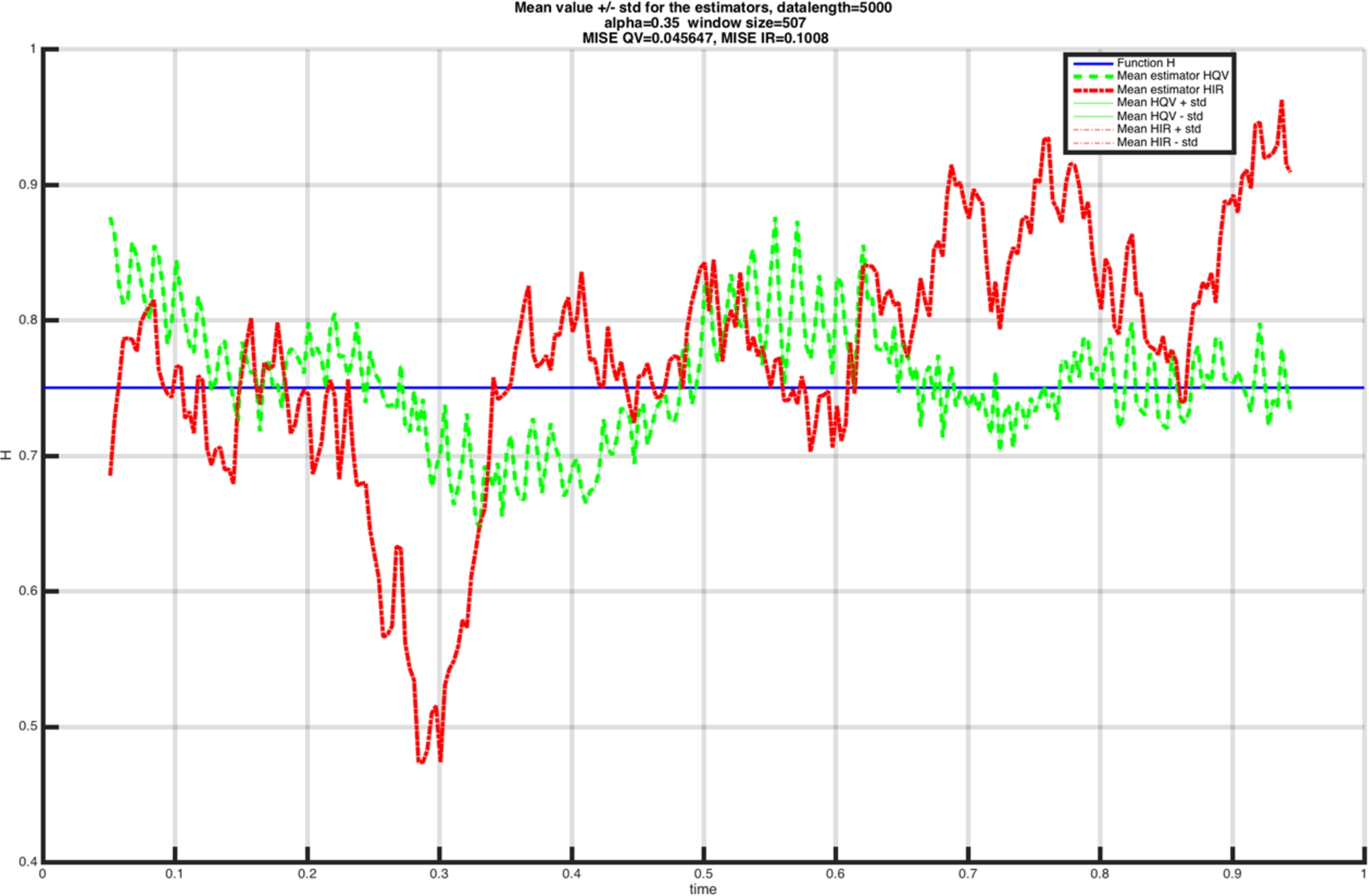
Mean estimation of constant function Hurst index
Mean estimation of Hurst index function
Let X be a fBm or a mBm. We observe one path of size n of the process X with mesh
It has been pointed in [12,24] that the localisation procedure of Hurst estimator adds a stochastic process to the right Hurst index
For Linear Regression of GQV and Increment Ratio Statistics, this sampling fluctuation has been proved through functional Central Limit Theorems (CLT) in [7,17,18].
(CLT Coeurjolly, 2005–2006 [17,18]).
Let X be a mBm with Hurst index
(CLT Bardet–Surgailis 2013 [7]).
Under some technical assumptions the functional CLT of Coeurjolly [
17
]
holds for both GQV and IR estimator, with two different limit processes
As a consequence of the functional CLT in [7,17], we can quote:
The speed of convergence is
The CLT’s in [7 ,17] explain the sampling fluctuation of the time-varying Hurst estimators for GQV and IRS, but we guess that the same kind of phenomenon remains in force for other estimators.
When we estimate a time-varying Hurst index
Fitting test
From the functional CLT (Theorem 2.4), we deduce the convergence of normalized square error as stated in the following Central Limit Theorem:
Under the assumptions of Theorem
2.4
, we have
The convergence in distribution with respect to the two parameters L and n means that the cumulative distribution function of the left hand is approximatively (up to ε) the one of standard Gaussian law, for L large enough and
Moreover,
and
By using Proposition 3.1, we can test if a time-varying Hurst index
Under the same assumptions and with the same notations as in Proposition
3.1
, we can test
Theorem 3.2 is a direct consequence of Proposition 3.1. The numerical simulations in Section 4 confirm the theorem. We give a sketch of the proof in the Appendix. □
Let us stress that we cannot calculate the power of the test since
The naive time-varying estimator
We successively test models extracted from the previous families. Those families of models are classified by order of complexity of function
Numerical simulations
A simulation must meet the following specifications: for a benchmark of time-varying Hurst indices
It is comfortable, but not essential, to have a small computing time. We have tested simulations by using Fractlab 2.2 and the code written by Jean-Marc Bardet [6,7] that we have improved for our study.
We test GQ estimator, decimated IRS2 estimators as in Bardet and Surgailis, (non decimated) IRS1 estimator and polynomial interpolation of (non decimated) IRS1.
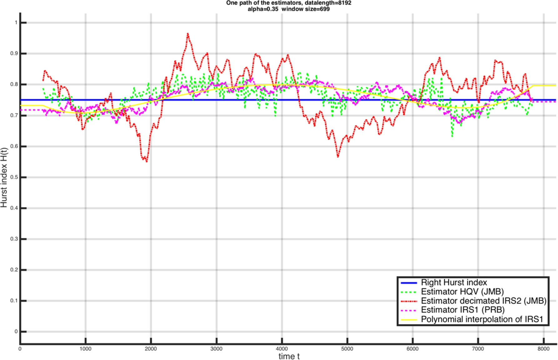
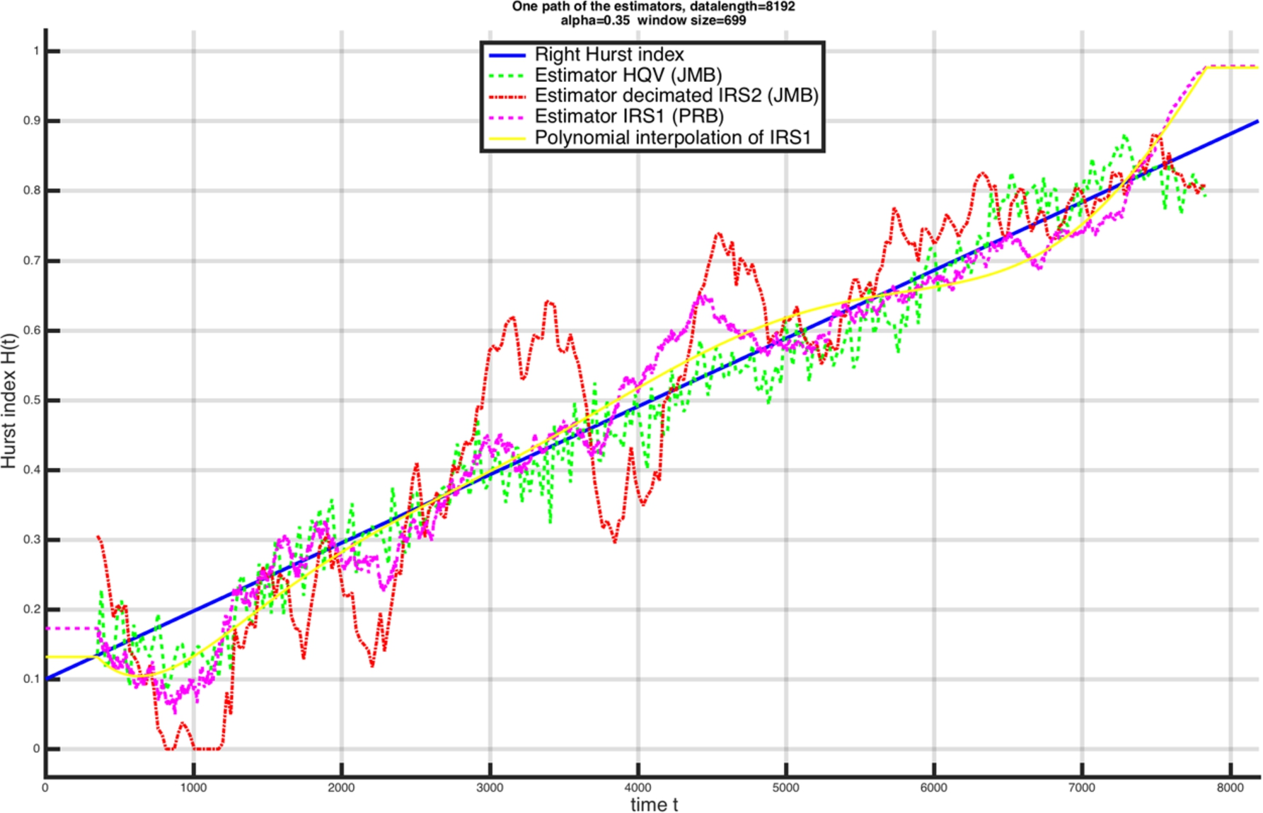
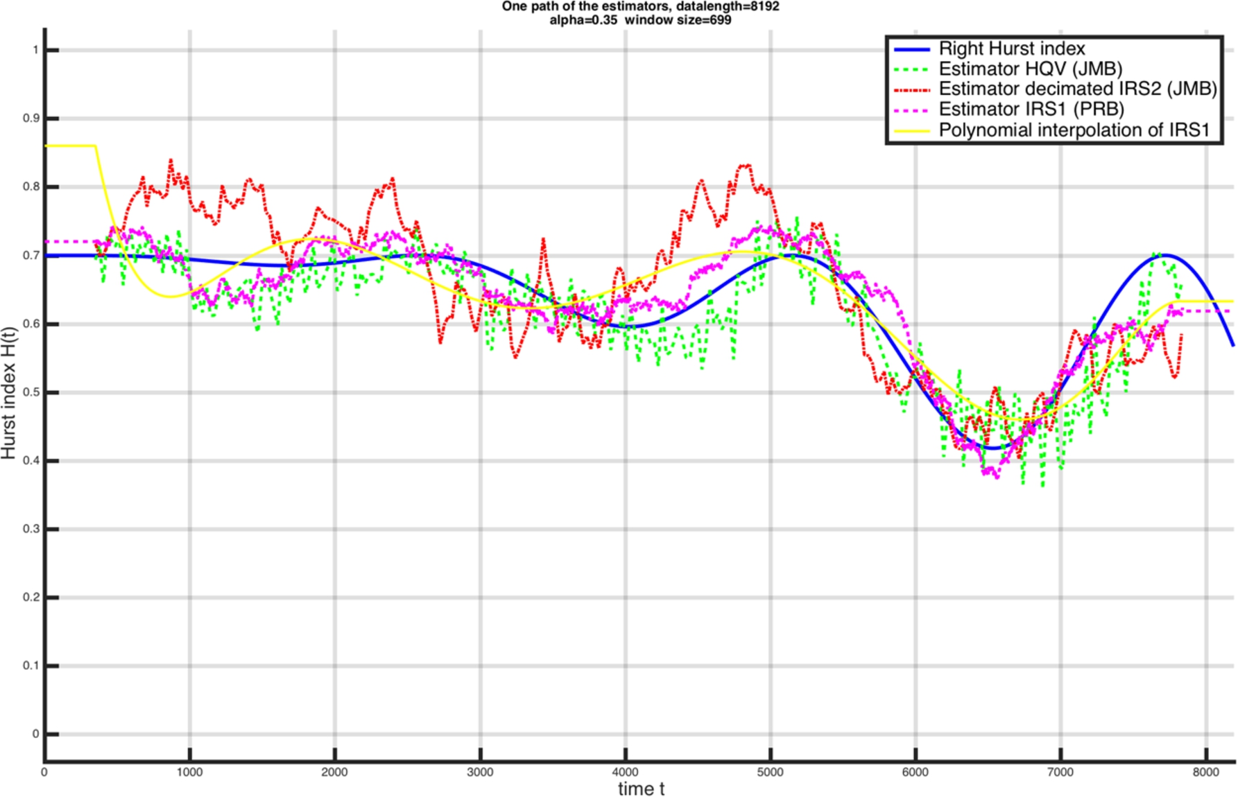
One path of the estimators for Hurst index
We note that the polynomial interpolation of the IRS estimator, for a single simulation (Fig. 5) or on average (Fig. 6), is the closest estimator to the right value of the Hurst index function. The IRS estimator alone is also a good approximation for the Hurst index despite fluctuations. The decimated IRS of Bardet [7] has a strong fluctuation that is larger than the Quadratic Variation estimator. Moreover, the curve of the polynomial interpolation of the IRS in yellow is the one that fluctuates the least compared to the other estimators.
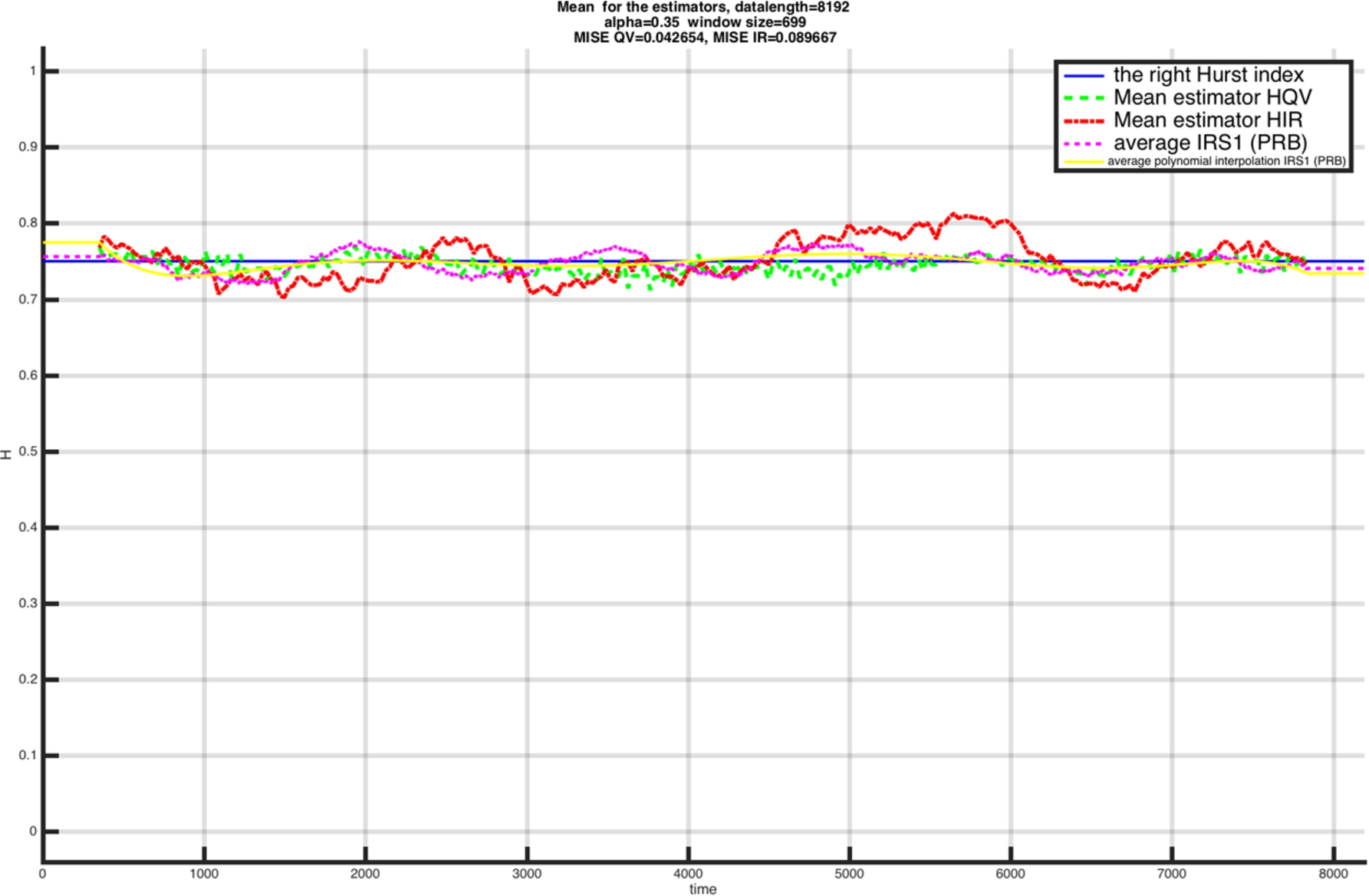
Average estimators for Hurst index
Next, we consider an affine function
One path of the estimators for Hurst index
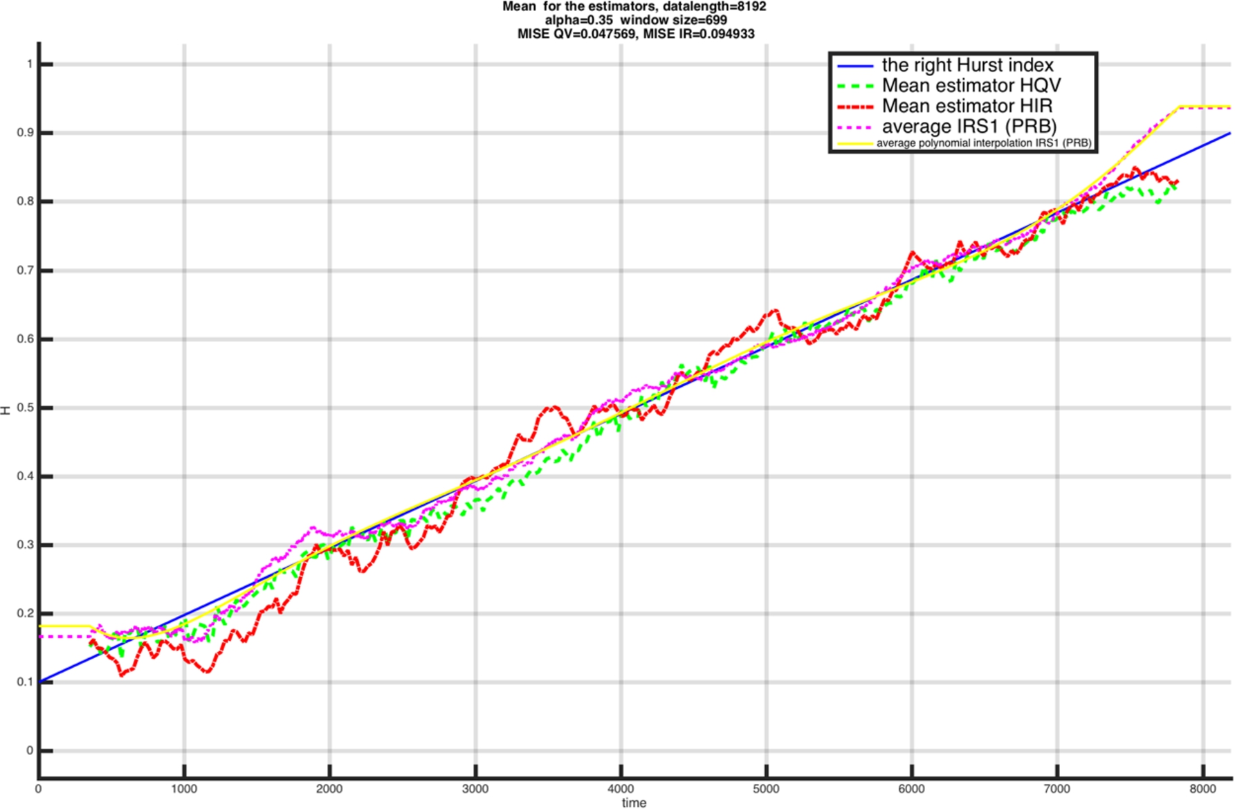
Average estimators for Hurst index
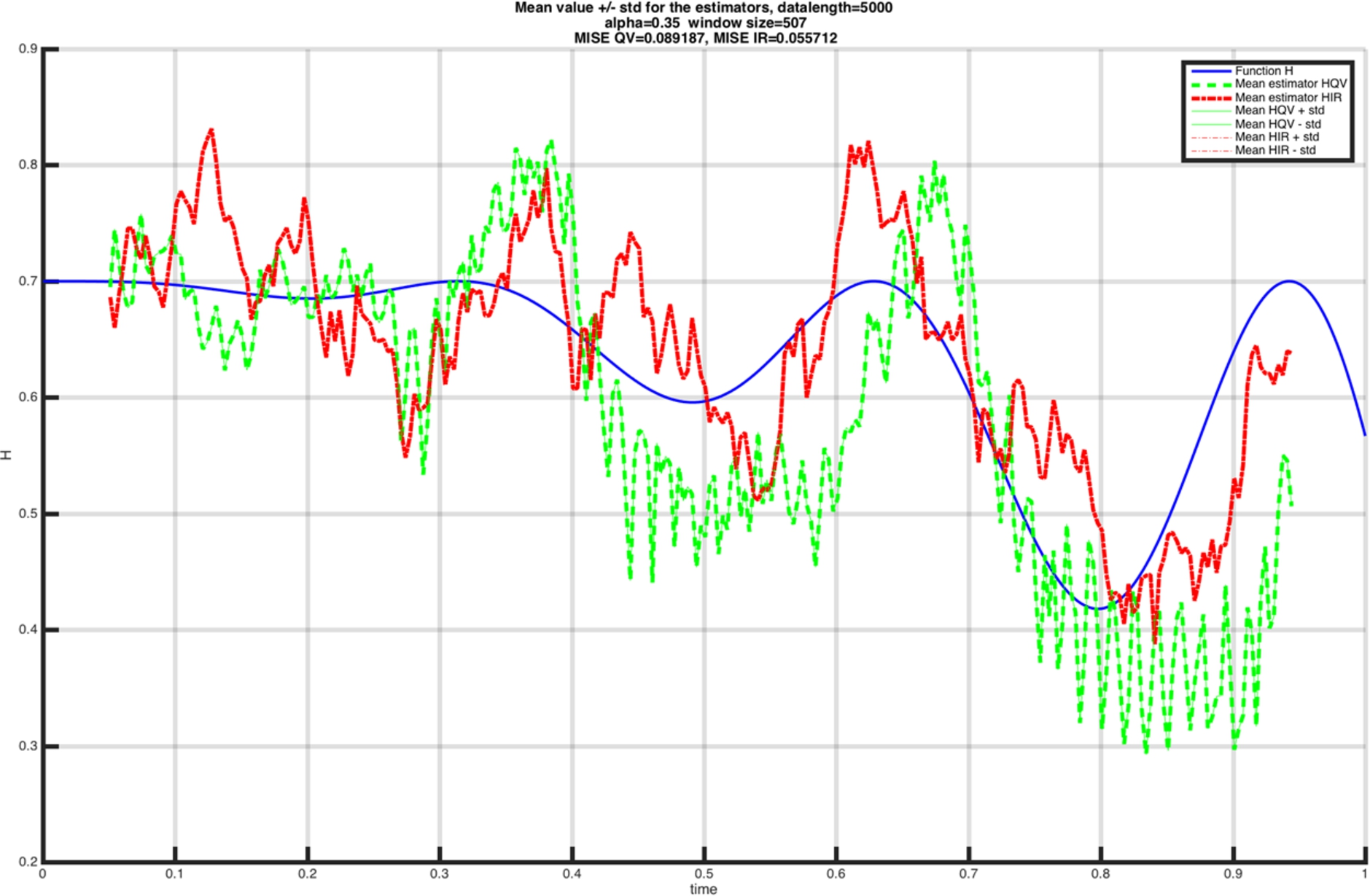
Eventually, we test on two sinusoidal functions
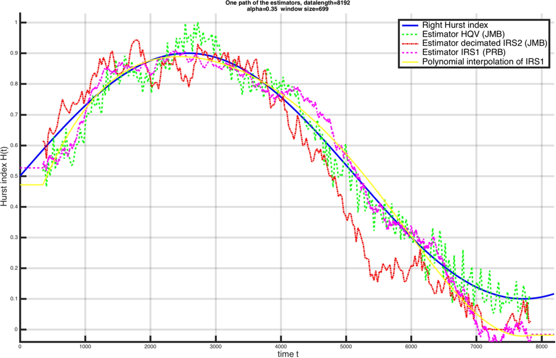
One path of the estimators for Hurst index
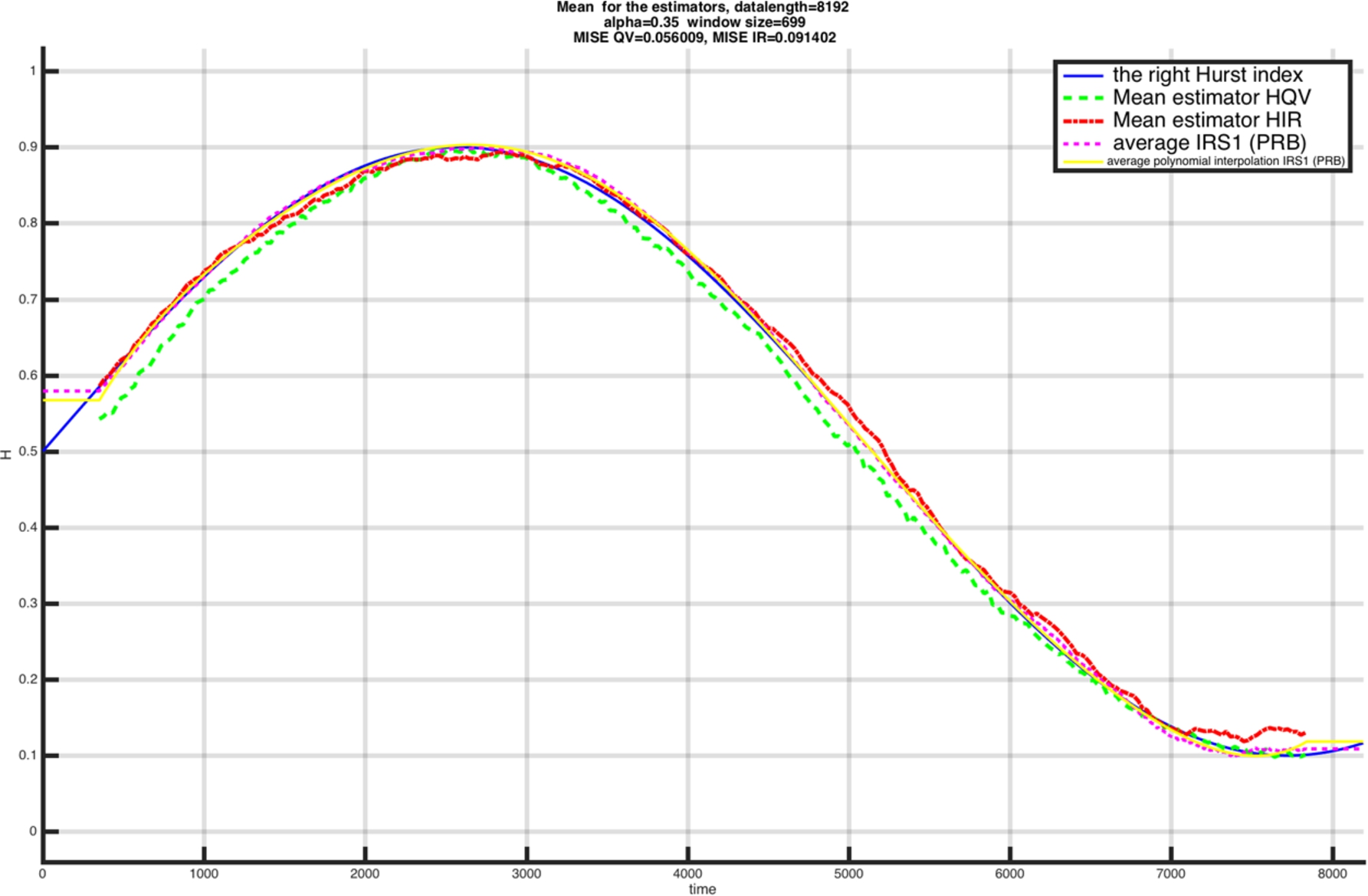
Average estimators for Hurst index
In the case of a single simulation, we notice that the polynomial interpolation of the IRS is the best estimator to approximate the right value of the Hurst index function
Then we calculate the bias and the Integrated Square Error (ISE) for each function, see e.g. Fig. 13 when
One path of the estimators for Hurst index
We remark that:
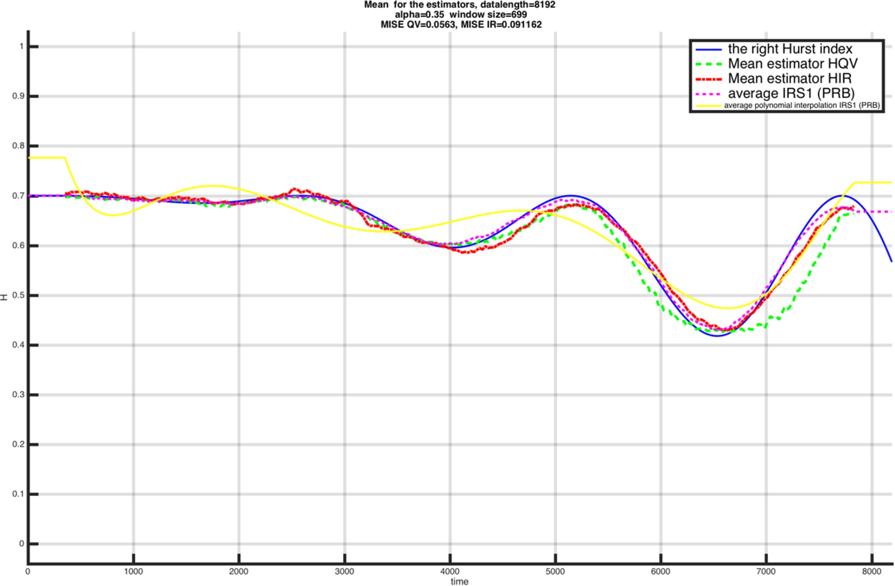
Average estimators for Hurst index
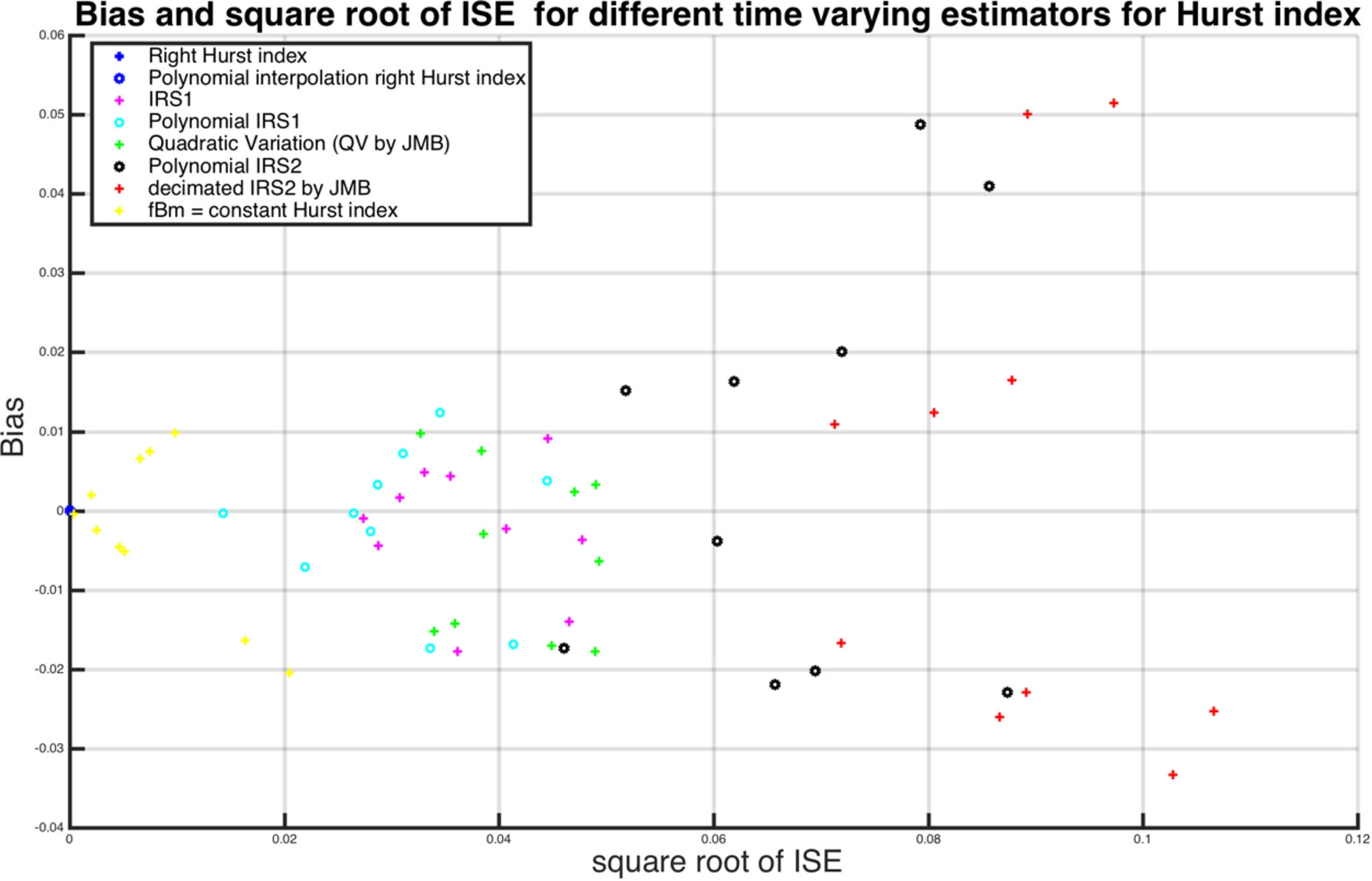
ISE vs Bias for different Hurst index estimators, when

ISE vs Bias for different Hurst index estimators, when
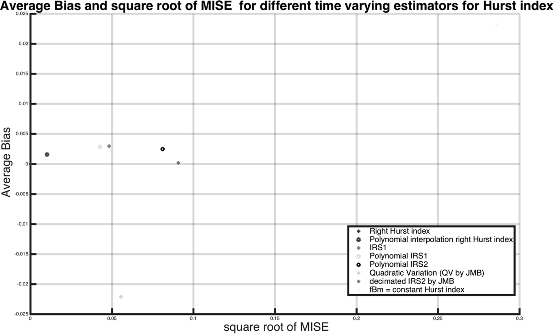
Average bias vs ISE or the different Hurst index estimators, when
When the Hurst index
Even when
All estimators always give wrong estimation of the regularity (or roughness) of
If we guess the good degree of interpolation, we would greatly reduce MISE.
Some applications outside finance
The multifractional Brownian motion (mBm) is hence defined from the fBm but with a time-varying Hurst index, which can be encountered in many different kinds of applications: In turbulence, Papanicolaou and Sølna [38] denote that “the power law itself [i.e. the Hurst index, …] and the multiplicative constant are not constants but vary slowly” in [38], whereas Lee [31] uses mBm with a regularly time-varying Hurst index for the air velocity, see [31, Fig. 5, p. 103]. Statistical study on magnetospheric dynamics points that an abrupt change in Hurst index can be observed a few hours before a space storm in solar wind [43]. In systems biology, [36] uses mBm to simulate molecular crowding that matches the statistical properties of sample data, whereas [33] uses mBm with piecewise constant Hurst index to model single file diffusion that is the motion of chemical, physical or biological particles in quasi-one-dimensional channel.
Applications in finance
Quantitative finance has been the most important field of application of both time series and stochastic processes for the last fifty years. The modern theory of modern finance is based on a fundamental concept defined by Fama [21]: the totality of available information is contained in market prices. New information will be immediately incorporated in the current prices. Fama distinguishes different form of market efficiency [22]. The informational efficiency could be strong when the set of information includes all the public and private information. A less restrictive notion is the semi-strong efficiency when the information set excludes the private information. But, the empirical tests aim to test a weak form of efficiency where the available information set includes only the past variations of the prices. The null hypothesis is hence the unpredictability of the future prices from the past prices [30]. The informational efficiency implies the impossibility from an agent to perform systematically better than the market. It is worth noting that this concept results from the combination of two economic hypotheses: (a) the rational expectation hypothesis according to which the agents use optimally the information and do not make systematic error [37] and (b) the market equilibrium condition: the observed price reflects the fundamental value of the asset. This last hypothesis could result from the great numbers of agents on the market (atomicity hypothesis). In other words, a market is efficient in the weakly form, if it is not possible to make (above average) profits (without accepting above average risk) by trading on the base of the past prices information set [34]. From an empirical point of view, the random walk hypothesis or the less restrictive martingale hypothesis is tested [28]. We refer to [32] for a survey of the different econometric methods.
The efficient market hypothesis [22] has lead to reject fBm as an admissible model for stock price. So, since the 1970’s, the use of martingale models with constant Hurst index
The main objection to fBm, as an admissible model for stock prices, is the existence of an arbitrage opportunity for such a fBm with a constant and known Hurst index. To put it in a nutshell, an arbitrage opportunity means the possibility of producing a positive return from zero investment by clever trading. For a fBm with known and constant Hurst index, it is possible to make an arbitrage, with a strategy based on infinitely small meshes of times and without transaction cost [16,41,42]. However, today the landscape has changed. The subprime mortgage crisis (2007–2009) recalled the limits of mainstream finance and reinforced the investigation of new or alternative models [40]. The probabilists has proved that as soon as there exist very small transaction costs, then arbitrage with fBm does no more exist [26,27]. Recent research in finance investigates pricing for fBm, see [19]. Then, modeling stock prices by mBm has been proposed. [24] pointed that there exists no arbitrage opportunity for such a mBm with a random time-varying Hurst index. Behavioral finance provides economic explanations: Market efficiency corresponds to
To sum up, new probabilist results show that fBm is an admissible model with transaction costs, statistics shows that mBm better fit the data and behavioral finance explains that under-reaction (
The next logical step for probability theorists would be to assume that the Hurst index is itself a stochastic process, that is to say with irregular paths, as the multifractional process with random exponent (MPRE) [5]. However, we show in this paper that this choice is counter productive as this complex model results from a statistical artifact.
We apply the test on financial data. The first application concerns the price of the NASDAQ (National Association of Securities Dealers Automated Quotations) of the US equity market (Fig. 16). We then aim at estimating the time varying Hurst index function for the NASDAQ with different estimators (Fig. 17): A piecewise constant function in magenta (see [8]), a mBm in green and a polynomial function of degree 9 in blue.
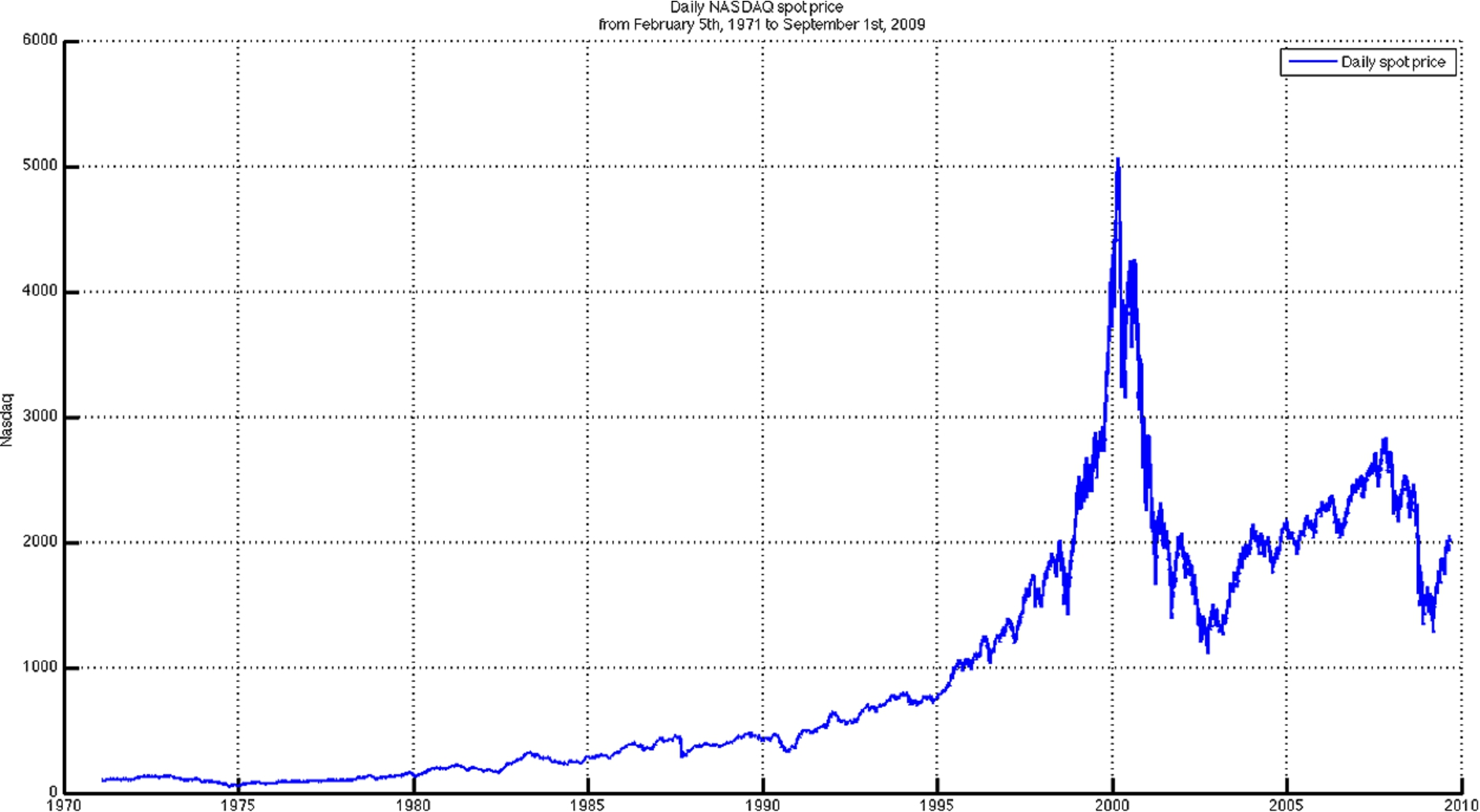
Daily NASDAQ spot price from February 1971 to September 2009.
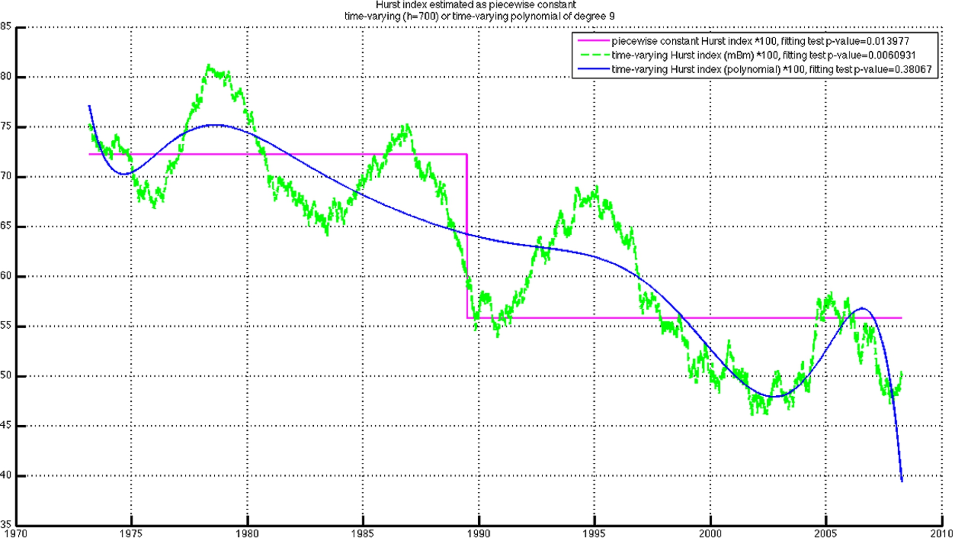
Different estimators for Hurst index for daily NASDAQ spot price.
The second application concerns the daily prices of West Texas Intermediate oil (WTI) from January 1986 until May 2016 (Fig. 18). We estimate Hurst index with the same estimators used in the precedent example (Fig. 19). For the oil price, we reject the second and the third estimator and we accept the model with a constant estimator with
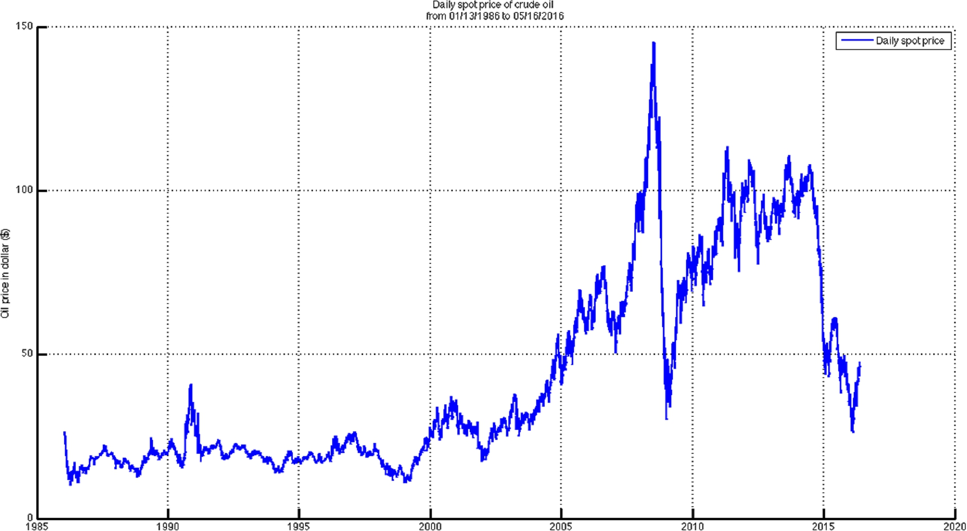
Daily price of the oil WTI.
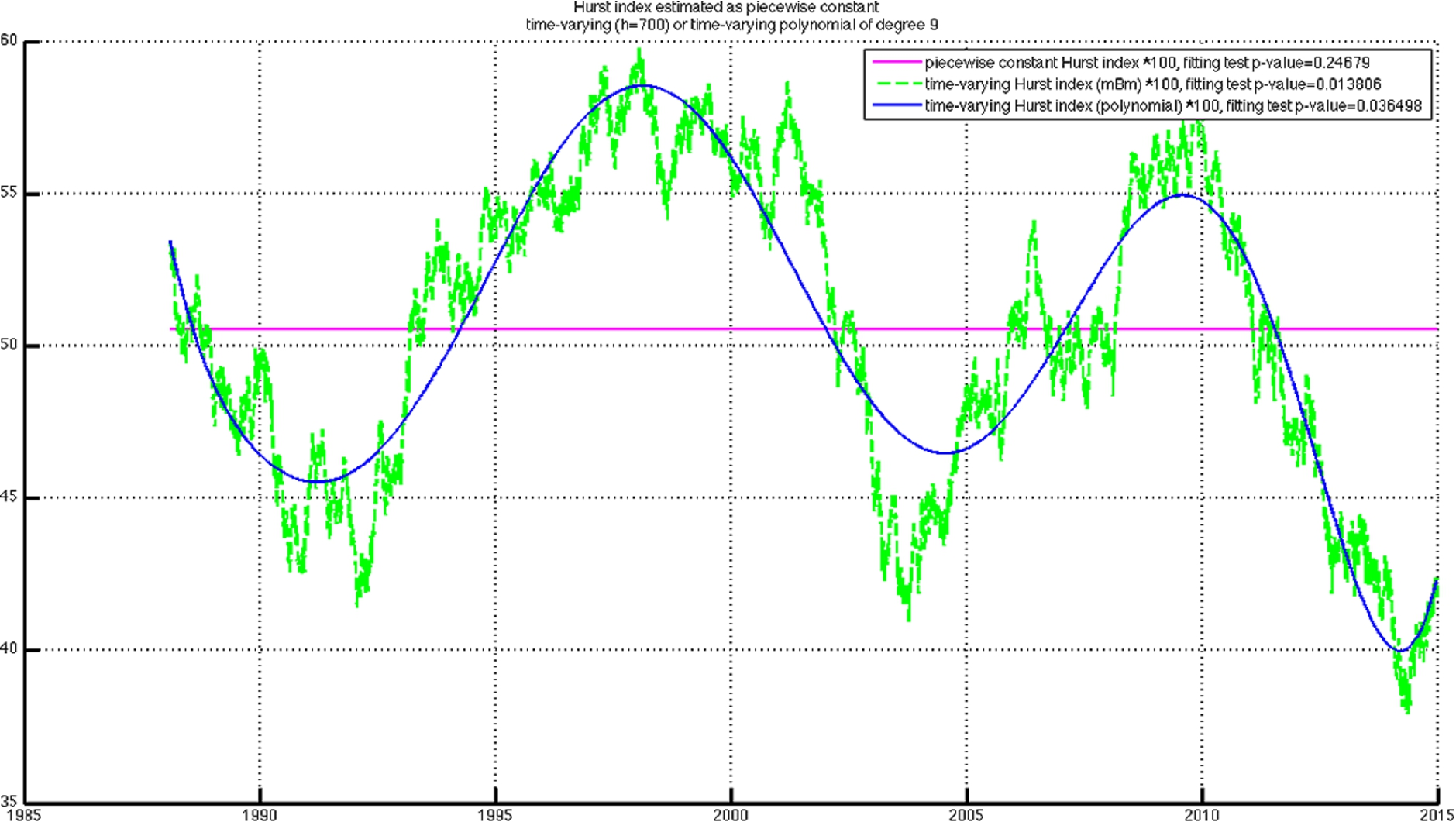
Three estimators for Hurst index for daily WTI price.
Two considered series illustrate time-varying Hurst index in financial market. They show very different patterns of the prices’ persistence.
The observation of the H index on the
A downward trend of the index, that goes from
A cyclical evolution of the H index, namely the recurrence of periods of market overreaction and under-reaction, which can probably be interpreted as the existence of misvaluation, at least in some segments of the market.
The most remarkable fact with regard to the crude oil market, is the cyclical nature of the H index around its efficiency value and the absence of any trend. Most of the studies do no reject the weak efficiency hypothesis. For instance, the results are in accordance with [3] which shows, using daily record of oil prices, that the crude oil market could be described by a random-walk process when short time scales are considered. Nevertheless, the topic is still a matter of debate, see e.g. [2].
The naive multifractional estimator
Footnotes
Acknowledgement
This research was supported by grant ANR-12-BS01-0016-01 “Do Well B.” (2012–2016) and by the project PEPS CNRS and Clermont-Ferrand Universities “Monitoring des états de stress”.
Proof of our main result – Theorem 3.2
For the sake of completeness, we recall the well-known lemma:
Preliminary remark. From Theorem 2.3 [17,18], we have the CLT (2.4). As pointed by Bardet–Surgailis [7], see e.g. Theorem 2.4, we also get a CLT for finite dimensional distribution, that is to say that for all finite family of times
Step 1. Let