An empirical study on using Hurst exponent estimation methods for pricing Call options by fractional Black

Abstract

This paper is an empirical study investigating the effect of using a fractional Black–Scholes model for pricing Call options in comparison to the classical Black–Scholes model. We estimate the Hurst parameter by nine different methods available in software R, for a set of fifteen assets from four different industries and for various lengths of used historical data. We use implied volatility for calculation of option price with a one month time to maturity. As a main result, we provide a table of tendencies of suitability for using each of the Hurst exponent estimation methods depending on the length of underlying data set.

Keywords

Call option fractional Black–Scholes model fractional Brownian motion Hurst exponent

1. Introduction

Assumptions of the standard Black–Scholes model [5] for option pricing have been relaxed in many ways. Approaches range from changing constant volatility to a time-dependent or a stochastic one [12], to changing the type of the underlying stock price process to more general processes, for example Lévy processes [2,10]. Fractional Brownian motion (fBm) is another concept for describing market behaviour and for modeling riskiness of assets, as proposed by Mandelbrot and Hudson [18]. This model used to be less popular in finance because it allows for arbitrage opportunities [4,7,27]. Hu and Øksendal [15] proved that arbitrage opportunities exist only if path-wise integration is used, but not with Itō type of stochastic integration. Other research showed that arbitrage opportunities disappear even if some small time is put between trading instead of continuous trading [23] or under transaction costs [14].

A difficulty with the fractional Black–Scholes option pricing model is that estimates of the Hurst exponent differ for different estimation methods. In [6], the authors calculate the Hurst exponent of financial time series by methods available in software R and test sensitivity of the results on the frequency of the time series. They conclude that the Hurst exponent of log-returns seems to grow with data frequency. In [16] they perform comparative analysis of statistical properties of the Hurst exponent estimators obtained by four different methods. They observed that: estimates of the Hurst exponent for stationary time series are biased normal random variables, with bias depending on the degree of self-similarity and on the length of the time series; standard deviations of the estimates depend on the method used and decrease with the growth of the series length. In [20], focusing on forecasting financial data, they observed that Hurst exponent estimates differ significantly for the full time series and for shorter time series, and that higher Hurst exponents of shorter time series lead to better trading profits than moving average based trading tool. European options in the fractional Brownian motion setting have been investigated in [20] by applying a risk preference based approach; the author provides a closed-form formula for European options within the fractional context. Some research has upgraded to using fractional stochastic volatility models for option pricing [8,9]. Empirical studies on fractional Black–Scholes model have been performed in literature across decades [17,25]. Currency options have been studied by means fBm in [26].

In this paper, we investigate the variability in Hurst estimates obtained by nine different methods available in software R and for various time series lengths (5 years, 2 years, 1 year, 6 months and 3 months), and draw conclusions in the environment of option pricing. In Section 2 we recall the definition and basic properties of fractional Brownian motion and the fractional Black–Scholes model for option pricing. Section 3 is dedicated to description of methodology and data used, and to vast numerical experiments followed by discussion. We draw observations about tendencies of suitability for each estimation method in terms of providing a best or a worst theoretical option price with respect to the length of date series used. This knowledge can be a helpful tool when facing decisions about which Hurst exponent estimation method to use in order to obtain a theoretical option price which best resembles its real future market value.

2. Résumé on fractional Brownian motion in option pricing

In this section we recall the definition and basic properties of fractional Brownian motion (fBm) as in [4]. We also recall formulas for the fractional Black–Scholes model for European Call option pricing.

2.1. Basic definition and properties of fBm

Definition 1.
A fractional Brownian motion ${B_{t}^{H}}_{t ⩾ 0}$ of Hurst index $H \in (0, 1)$ is a continuous and centered Gaussian process with covariance function $\begin{matrix} E [B_{t}^{H} B_{s}^{H}] = \frac{1}{2} (t^{2 H} + s^{2 H} - | t - s |^{2 H}) . \end{matrix}$

Basic properties of fBm include: $E [B_{t}^{H}] = 0$ and $E [{(B_{t}^{H})}^{2}] = t^{2 H}$ for all $t ⩾ 0$ ; $B_{t}^{H}$ has homogeneous increments; $B_{t}^{H}$ has continuous trajectories; for $H = \frac{1}{2}$ , fBm is the standard Brownian motion. An important property of fBm is its long-range dependence, distinguishing two classes of time series [24]: for $H > \frac{1}{2}$ , the increments of the underlying random process are positively correlated and the process is called persistent (and tends to follow a drift); for $H < \frac{1}{2}$ , the increments are negatively correlated and the process is called anti-persistent (e.g. mean-reverting processes). For $H = \frac{1}{2}$ , the increments are independent. According to Qian and Rasheed [22], most economic and financial processes are persistent.

Table 2
Time spans of historical data used

Time span Dates Length of log-returns series

Five years (5Y) Dec 13, 2011–Dec 12, 2016 1257

Two years (2Y) Dec 1, 2014–Dec 12, 2016 $512 = 2^{9}$

One year (1Y) Dec 14, 2015–Dec 12, 2016 251

Six months (6M) June 10, 2016–Dec 12, 2016 $128 = 2^{7}$

Three months (3M) Sept 12, 2016–Dec 12, 2016 $64 = 2^{6}$

2.2. fBm in pricing Call options

Time span	Dates	Length of log-returns series
Five years (5Y)	Dec 13, 2011–Dec 12, 2016	1257
Two years (2Y)	Dec 1, 2014–Dec 12, 2016	$512 = 2^{9}$
One year (1Y)	Dec 14, 2015–Dec 12, 2016	251
Six months (6M)	June 10, 2016–Dec 12, 2016	$128 = 2^{7}$
Three months (3M)	Sept 12, 2016–Dec 12, 2016	$64 = 2^{6}$

In the fractional Black–Scholes model, the price of the underlying asset $S_{t}$ follows the stochastic equation $\begin{matrix} (1) & S_{t} = S_{0} e^{(μ t + σ B_{t}^{H} - \frac{1}{2} σ^{2} t^{2 H})}, \end{matrix}$ where $B_{t}^{H}$ is a fBm with Hurst index H, $S_{0}$ is an initial price, μ is the average return, σ is the volatility of log-returns. Price V at time t of a Call option with expiry in time T and strike price K for stock price S is given by $\begin{array}{l} V (S, t; K, r, T, σ, H) \\ (2) & = S N (d_{1}) - K e^{- r (T - t)} N (d_{2}), \end{array}$ where r is the risk-free interest rate and the arguments of the cumulative standard normal distribution function $N (\cdot)$ are $\begin{matrix} (3) & d_{1, 2} = \frac{ln \frac{S}{K} + r (T - t) \pm \frac{1}{2} σ^{2} (T^{2 H} - t^{2 H})}{σ \sqrt{T^{2 H} - t^{2 H}}}; \end{matrix}$ see [15 ,21] for derivation. This formula holds for $H \in (0, 1)$ and is derived using the Wick–Itō–Skorohod type of integration ensuring arbitrage-free market.

2.3. Note on volatility

For the standard Black–Scholes (BS) model, volatility is usually constant and estimated as the standard deviation of log-returns. In more advanced models, it can be time-dependent or even stochastic. In fractional Black–Scholes (fBS) models, authors in [19] consider constant as well as stochastic volatility, in [29] they use constant volatility calculated in a standard way as the standard deviation of historical data, in [3] they discuss the possibility to use short-rate models and volatility models based on fractional Ornstein–Uhlenbeck processes. Authors in [13] consider volatility processes which reveal long- and short-range dependence. In [11], authors provide a discussion about relationship of the standard BS volatility and fractional BS volatility. Last, authors in [1] compute implied volatility.

In order to eliminate “imperfections” of volatility models which could manipulate our comparison of different methods, we use implied volatility in this paper. Implied volatility obtained from fractional Black–Scholes model in which all parameters are annualized is annualized as well. Therefore we do not need to perform annualization, but if it would be needed, the relationship between daily volatility $σ_{day}$ and yearly $σ_{year}$ is $σ_{year} = σ_{day} 252^{H}$ .

3. Numerical experiments

We shall work with nine methods available in software R: R/S Rescaled Range Statistic method (RS), Aggregated Variance Method (VAR), Aggregated Absolute Value/Moment Method (AVM), Peng’s or Variance of Residuals Method (VRM), Periodogram Method (PER), Differenced Aggregated Variance Method (DVAR), Higuchi’s or Fractal Dimension Method (HIG), Boxed/Modified Periodogram Method (BPER), and Wavelet Method (WAV). We estimate the Hurst exponent for a set of fifteen assets by each of these methods. As it will be shown, the results differ for different methods or for different lengths of underlying time series. fBm usually yields better theoretical option prices than the standard Brownian motion model, as we shall see. The methods are described in [28] and other literature.

3.1. Data and methodology

We selected stocks from four different areas of business: banking, IT, industry and energetics; see Table 1.

Table 1
Assets

Group Sector Assets

1 banking HSBC, JPM, BAC, DB

2 IT GOOG, AAPL, MSFT, IBM

3 industry TM, HMC, CAH, MT

4 energetics XOM, BP, PTR

Group	Sector	Assets
1	banking	HSBC, JPM, BAC, DB
2	IT	GOOG, AAPL, MSFT, IBM
3	industry	TM, HMC, CAH, MT
4	energetics	XOM, BP, PTR

As knowing the right length of historical time series to be used in financial computations is sometimes almost alchemy, we shall examine very short, medium, as well as relatively long time series in this paper; see Table 2. We shall also test importance of the length of the log-returns series for being or not being a power of 2 (as this is recommended by some of the methods for estimating H).

For estimating H of log-returns series, we used default parameter values, as suggested by R. Changing these parameters may significantly change the estimates of H and we wanted to eliminate different skills of different investors. To summarize these default parameters, we copy the relevant part of R commands for each of the estimation methods used:

rsFit(x$V1, levels = 50, minnpts = 3, cut.off = 10^c(0.7, 2.5))aggvarFit(x$V1, levels = 50, minnpts = 3, cut.off = 10^c(0.7, 2.5))absvalFit(x$V1, levels = 50, minnpts = 3, cut.off = 10^c(0.7, 2.5), moment = 1)pengFit(x$V1, levels = 50, minnpts = 3, cut.off = 10^c(0.7, 2.5), method = c("mean", "median"))perFit(x$V1, cut.off = 0.1, method = c("per", "cumper"))diffvarFit(x$V1, levels = 50, minnpts = 3, cut.off = 10^c(0.7, 2.5))higuchiFit(x$V1, levels = 50, minnpts = 2, cut.off = 10^c(0.7, 2.5))boxperFit(x$V1, nbox = 100, cut.off = 0.10)waveletFit(x$V1, length = NULL, order = 2, octave = c(2, 8))

Calculating implied volatility is directly connected to calculating option price and comparing it to available market data. After we get the implied volatility for option market price from “yesterday”, we can proceed to calculating current option price. The procedure is described in Algorithm 1.

Algorithm 1

Calculating implied volatility and option price

Table 3 contains the initial asset prices $S_{1}$ (as of Dec 9, 2016), $S_{0}$ (as of Dec 12, 2016) and the options’ strike prices K for each asset. Expiry is approximately in 1 month (on Jan 20, 2017), hence $T_{0} = 27 / 252$ years and $T_{1} = 28 / 252$ for calculating implied volatility in Step 7 of Algorithm 1. We used risk-free interest rate $r = 0.48 %$ p.a., which was the 3-month American bond return according to finance.yahoo.com/bonds as of Dec 13, 2016, so we used it as a best approximation of one-month rate.

Table 3

Adjusted close stock prices needed for option pricing. Selected strike prices K for Call options with maturity on Jan 20, 2017

3.2. Numerical results and discussion

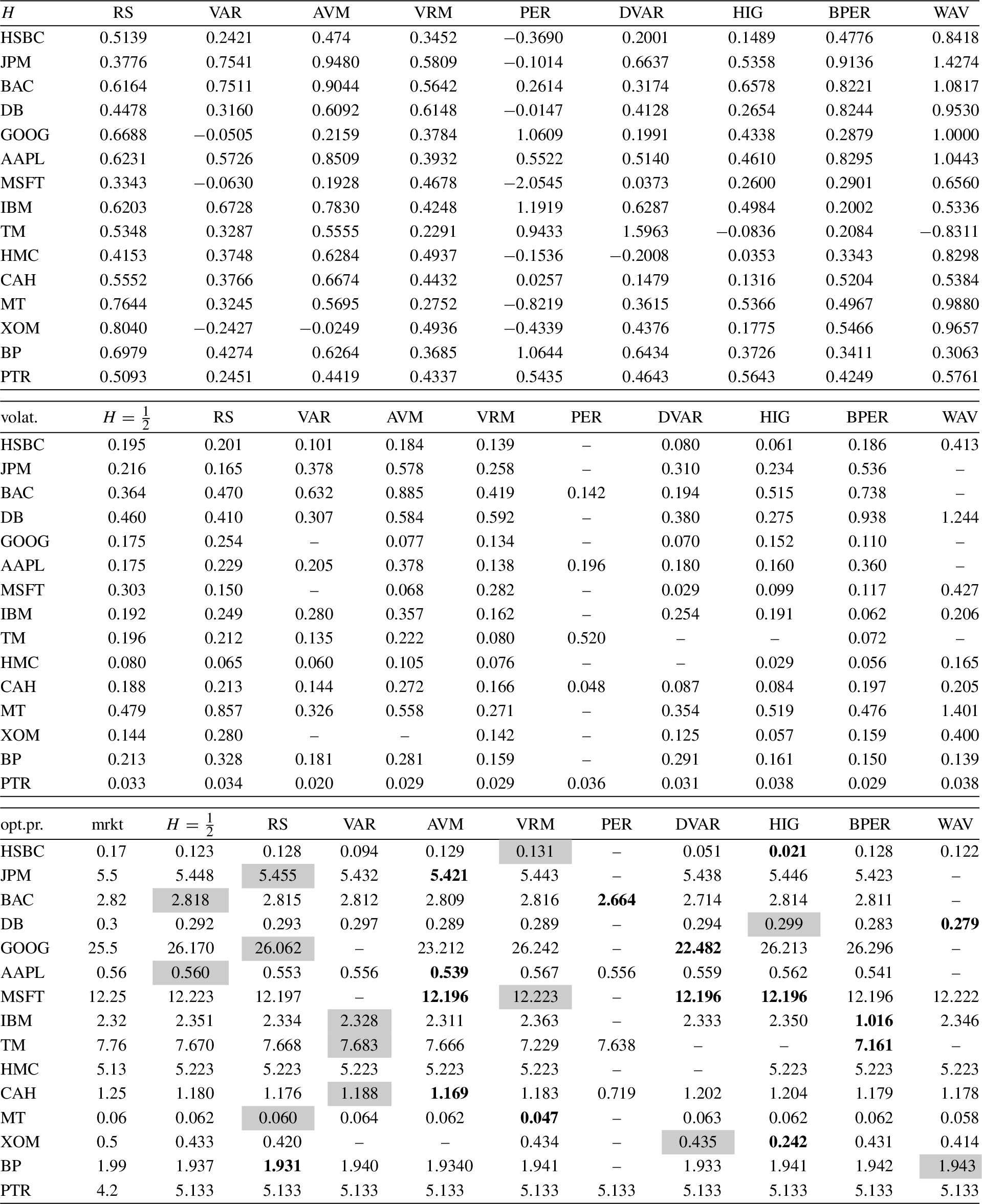
We performed computations for all time spans mentioned in Table 2. Tables 6–10 summarize the results for 5 years, 2 years, 1 year, 6 months and 3 months of historical data, respectively. Top tables show estimated Hurst exponents by all of the considered estimation methods, middle tables contain corresponding implied volatilities and bottom tables calculated option prices. We depict estimates of H for two assets in Fig. 1. 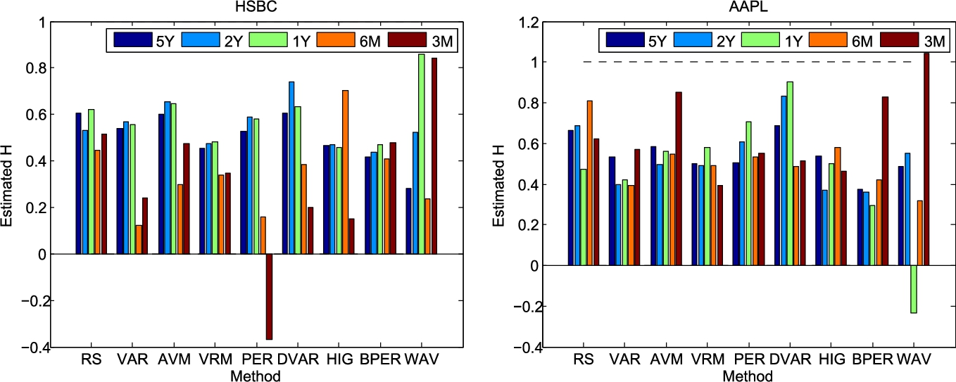For informative and learning purposes, we also calculated implied volatilities for the entire span of $H \in (0, 1)$ and depict them for each asset in Fig. 2.

Fig. 1.

Estimates of H for selected assets, for all considered methods and historical data time spans.

Fig. 2.

Implied volatility for all 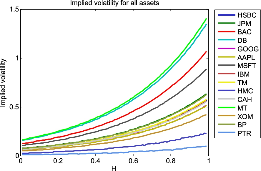$H \in (0, 1)$ , all assets.

Before proceeding to discussing the results, let us first summarize the main message obtained from our experiments. Table 4 gives an overview of success rate of each estimation method in terms of yielding the best or the worst theoretical option price compared to real market price and Table 5 summarizes the tendencies and suitability of using individual estimation methods for different data set lengths. We defined their classification as good, good/neutral, neutral, bad/neutral and bad, depending on the difference between the number of best and worst option prices yielded for the given data set length for the 15 test assets and from all used methods. A special result was obtained for DVAR, which is significantly worse for 5Y and 2Y data than any other method is abd for any other data length. Similarly, BPER is positively outstanding for 2Y data. The rest of the results for other methods reveal good or bad suitability in a more mild extent.

Another major conclusion we can draw from our experiments is depicted in Fig. 2. It is apparent that implied volatility is an increasing function of H and the curves for individual assets seem to be ordered in a non-intersecting way.

Table 4

Rate of success for tested estimation methods in terms of the number of best and worst theoretical option price values yielded by the corresponding method and data set length

Data set	5Y		2Y		1Y		6M		3M

	best	worst	best	worst	best	worst	best	worst	best	worst
$H = 1 / 2$	1×	–	1×	1×	1×	–	2×	–	2×	–
RS	3×	3×	–	–	2×	1×	1×	2×	3×	1×
VAR	1×	1×	3×	1×	1×	4×	2×	4×	3×	–
AVM	1×	–	1×	–	2×	2×	2×	–	–	4×
VRM	–	–	–	–	1×	–	1×	–	2×	1×
PER	–	–	1×	2×	1×	1×	2×	1×	–	1×
DVAR	–	5×	2×	7×	1×	3×	1×	–	1×	2×
HIG	–	–	–	–	4×	–	–	1×	1×	3×
BPER	4×	2×	7×	1×	1×	–	1×	1×	–	2×
WAV	3×	1×	–	1×	–	2×	1×	4×	–	1×

Table 5

Tendencies of suitability of the estimation methods based on the number of best and worst theoretical option price values for different data set lengths. Good: difference of at least two best results out of all the methods; good/neutral: one more best result than worst results; neutral: same number of best and worst results; bad/neutral: one more worst result than best results; bad: at least two more worst results than best results

Data set	5Y	2Y	1Y	6M	3M
$H = 1 / 2$	good/neutral	neutral	good/neutral	good	good
RS	neutral	neutral	good/neutral	bad/neutral	good
VAR	neutral	good	bad	bad	good
AVM	good/neutral	good/neutral	neutral	good	bad
VRM	neutral	neutral	good/neutral	good/neutral	good/neutral
PER	neutral	bad/neutral	neutral	good/neutral	bad/neutral
DVAR	bad	bad	bad	good/neutral	bad/neutral
HIG	neutral	neutral	good	bad/neutral	bad
BPER	good	good	good/neutral	neutral	bad
WAV	good	bad	bad	bad	bad/neutral

The other observations we can do from Tables 6, 7, 8, 9 and 10 are the following:

With shortening the underlying log-returns series, there is an increasing number of estimates of H with values out of range $(0, 1)$ . This can happen because the methods estimate H as a slope of a regression line, which clearly can attain values negative or greater than one; see the R manual1

https://r-forge.r-project.org/scm/viewvc.php/*checkout*/pkg/fSeries/chm/3A-LongRangeDependence.html?revision=628&root=rmetrics&pathrev=650

or corresponding literature for more details. We consider these estimates as invalid, as they do not have any meaning in regard to the definition (where

H \in (0, 1)

) or natural fractal dimension boundaries (fractions between integer dimensions must be less than one and greater than zero). We can see that for 5Y or 2Y data there is no such problem; for 1Y data there are 3 such cases, for 6M there are 7 and for 3M there are 22 such cases out of 135. Methods most sensitive to the length of time series appear to be (in decreasing order): PER (11 results out of range), WAV (9), VAR (5), DVAR (5), AVM (3), HIG (1). Methods RS, VRM and BPER never had this problem, so they seem to be most robust. We can see that their results for 2Y and 1Y are mutually quite consistent and in the “healthy” range (away from ends of the definition interval for H and similar to estimates from other methods which are not apparent outliers), but for 6M and 3M some outliers show up: for example, for asset JPM and method BPER we have

H = 0.5664

from 6M data and

H = 0.9136

for 3M data, while for longer data the estimates were around 0.3–0.4. Similarly, for asset XOM and method RS, we have

H > 0.8

for 6M and 3M data, while for longer time series we have

H \sim 0.4 – 0.5

. This shows that one has to be cautious with using shorter time series, even if the estimates of H might seem alright at first glance.

Quality of results does not apparently depend on whether the underlying time series is or is not of a length of a power of two.

Implied volatilities corresponding to estimated H attain “standard” volatility values of around 0.2 typical for log-returns of assets, with the exception of assets HMC and PTR where they are often less than 0.1. This holds regardless of the different data time spans. If we estimate volatility of these assets as standard deviation from data (annualized by formula mentioned at the end of Section 2.3), we get values typically around 0.2, which indicates that the corresponding option’s market price is not right, which then yields strange implied volatilities. As we will see in Point f), calculated option prices of these two assets behave strangely as well.

Calculated option prices for assets HMC and PTR differ among different estimation methods on 11th or later decimal places, and therefore seem to be the same, regardless of estimation method or time span of data. These are the two assets from Point d) with strange implied volatility.

Most of the time, fBS model outperforms the standard BS option pricing model. Sometimes, the standard BS model yields best option prices, outperforming any of the fBS models.

4. Conclusions

We took a closer look at the possibility of using fractional Brownian motion in financial practice of option pricing. On a set of fifteen assets representing different industries, we compared nine methods available for Hurst index estimation in statistical software R. We provided a useful table with tendencies to provide best, worst or mediocre theoretical option prices for each of the methods and each considered data length. We also observed that the fractional Black–Scholes model usually but not always provides a better theoretical option price than the standard Black–Scholes model. We used implied volatility in our computations in order to eliminate effects of different volatility models. Implied volatility of two of the assets were very small, which resulted in inaccurate option prices. That may be a sign of wrong market price of these options. In this paper, we used default parameter values of the estimation methods as suggested by R software, in order to represent a simple investor not changing any parameters. Optimization of parameters for all or any of the estimation methods can be inspiration for future research.

Footnotes

Acknowledgements

The authors were supported by VEGA 1/0062/18 grant and DAAD-Ministry of Education of Slovak republic grant ENANEFA.

Table 10

Hurst exponent estimates, corresponding implied volatility, and calculated theoretical option price for 3M data. Option prices which are closest to the market (mrkt) price (as of Dec 12, 2016) are highlighted in a gray cell, and prices which are farthest away from the market price are marked in bold. All results are displayed rounded to 4 or 3 decimal places due to page width

References

Ballestra

L.V.

and Cecere

, A numerical method to compute the volatility of the fractional Brownian motion implied by American options, International Journal of Applied Mathematics26(2) (2013), 203–220. doi:10.12732/ijam.v26i2.7.

Barndorff-Nielsen

O.E.E.

Mikosch

T.E.

and Resnick

S.I.E.

, Lévy Processes: Theory and Applications, Springer, 2001.

Bender

and Viitasaari

, Fractional Brownian Motion in Financial Modeling. Wiley StatsRef: Statistics Reference Online, (2016), 1–5.

Biagini

Øksendal

and Zhang

, Stochastic Calculus for Fractional Brownian Motion and Applications, Springer, 2008.

Black

and Scholes

, The pricing of options and corporate liabilities, The Journal of Political Economy81(3) (1973), 637–654. doi:10.1086/260062.

Brania

and Gurgul

, The impact of estimation methods and data frequency on the results of long memory assessment, Managerial Economics16(1) (2015), 7–37. doi:10.7494/manage.2015.16.1.7.

Cheridito

, Arbitrage in fractional Brownian motion models, Finance and Stochastics7(4) (2003), 533–553. doi:10.1007/s007800300101.

Comte

Coutin

and Renault

, Affine fractional stochastic volatility models, Annals of Finance8(2) (2012), 337–378. doi:10.1007/s10436-010-0165-3.

Comte

and Renault

, Long-memory in continuous-time stochastic volatility models, Mathematical Finance8 (1998), 291–323. doi:10.1111/1467-9965.00057.

10.

Cont

and Tankov

, Financial Modelling with Jump Processes, Chapman and Hall/CRC Financial Mathematics Series, 2003.

11.

Flint

and Mare

, Fractional Black–Scholes Option pricing, Volatility Calibration and Implied Hurst Exponents, 2016, 10 June 2016, available at: https://papers.ssrn.com/sol3/papers.cfm?abstract_id=2793927.

12.

Fouque

J.P.

Papanicolaou

and Sircar

K.R.

, Derivatives in Financial Markets with Stochastic Volatility, Cambridge University Press, 2000.

13.

Garnier

and Sølna

, Correction to Black–Scholes Formula due to Fractional Stochastic Volatility, 2015, 3 Sep 2015 arXiv:1509.01175v1 [q-fin.MF].

14.

Guasoni

, No arbitrage under transaction costs, with fractional Brownian motion and beyond, Mathematical Finance16(3) (2006), 569–582. doi:10.1111/j.1467-9965.2006.00283.x.

15.

and Øksendal

, Fractional White Noise Calculus and Applications to Finance, Infin. Dimens. Anal. Quantum. Probab. Relat. Top.6(1) (2003). doi:10.1142/S0219025703001110.

16.

Kirichenko

Radivilova

and Deineko

, Comparative Analysis for Estimating of the Hurst Exponent for Stationary and Nonstationary Time Series, International Journal Information Technologies & Knowledge5 (2011).

17.

Mandelbrot

B.B.

, Fractals and Scaling in Finance, Discontinuity, Concentration, Risk, Springer, 1997.

18.

Mandelbrot

B.B.

and Hudson

R.L.

, The (Mis)Behavior of Markets: A Fractal View of Risk, Ruin and Reward, Profile Books, 2008.

19.

Mishura

, Fractional stochastic integration and Black–Scholes equation for fractional Brownian model with stochastic volatility, Stochastics and Stochastic Reports76(4) (2007).

20.

Mitra

S.K.

, Is Hurst Exponent Value Useful in Forecasting Financial Time Series?, Asian Social Science8(8) (2012).

21.

Necula

, Option pricing in a fractional Brownian motion environment, Mathematical Report6(3) (2004).

22.

Qian

and Rasheed

, Hurst exponent and financial market predictability, in: Proceedings of the 2nd IASTED International Conference of Financial Engineering and Applications, Cambridge, MA, USA, 2004, pp. 203–209.

23.

Rostek

, Option Pricing in Fractional Brownian Markets, Lecture Notes in Economics and Mathematical Systems, Vol. 622, Springer, 2009.

24.

Sarkar

, Fractional Brownian Motion: Long range dependency, Markov property, Simulation strategy, A review, 2008.

25.

Shiryaev

A.N.

, Essentials of Stochastic Finance: Facts, Models, Theory, World Scientific, 1999.

26.

Shokrollahi

and Kiliçman

, The valuation of currency options by fractional Brownian motion, SpringerPlus5 (2016), 1145. doi:10.1186/s40064-016-2784-2.

27.

Sottinen

and Valkeila

, On arbitrage and replication in the fractional Black–Scholes pricing model, Statistics & Decisions21 (2003), 137–151.

28.

Taqqu

M.S.

and Teverovsky

, On estimating the intensity of long-range dependence in finite and infinite variance time series, in: A Practical Guide to Heavy Tails: Statistical Techniques and Applications Adler

R.J.

et al., eds, Birkhäuser, Boston, 1998, pp. 177–217.

29.

Zhou

, The application of fractional Brownian motion in option pricing, International Journal of Multimedia and Ubiquitous Engineering10(1) (2015), 173–182. doi:10.14257/ijmue.2015.10.1.16.

An empirical study on using Hurst exponent estimation methods for pricing Call options by fractional Black–Scholes model