RFID software-based shielding: Implementation of further approaches under varying surrounding conditions

Abstract

Given the promising results obtained by the Software-Based Shielding (SBS) in our previous work entitled “Software-based shielding for real-time inventory count in different store areas: a feasibility analysis in fashion retail”, in this paper, we go into more detail by exploring the effect of certain surrounding aspects, such as (i) the partition wall, and (ii) the density of tags. We also propose alternative algorithms other than logistic regression analysed in the previous work –i.e., a heuristic algorithm, a Neural Network (NN), a Convolutional Neural Network (CNN), and the introduction of reference tags to enhance these approaches. The results show that the logistic regression and the CNN are the most accurate models. The choice between them might depend on the application context: the first is less reliable but much simpler to implement, while the second is a more complex and complete machine learning model. Concerning the environmental conditions, the density and disposition of RFID tags appear the aspects with the greatest impact.

Keywords

RFID software-based shielding fashion retail machine learning algorithms

1 Introduction

Radio Frequency IDentification (RFID) is an established and well-known technology that has proven its effectiveness in automating processes and increasing their accuracy along the supply chain of several different industries (Abugabah et al., 2020; Esposito et al., 2015; Vivaldi et al., 2020). The last decades have seen a general shift of the level of tagging: from the pallet- or case-level tagging of the ‘90s and of early 2000s, we have recently experienced an ever-growing increase of item-level tagging deployments. Item-level tagging, in fact, has demonstrated to be very effective in improving inventory accuracy, reducing out-of-stock, and enabling omnichannel retailing (Goyal et al., 2016; Hardgrave, 2012). Thus, the application of item-level tags has started from some forerunners industries and companies, especially in the fashion and apparel sector (Cilloni et al., 2019; Solti et al., 2018), and it has moved to other supply chains, such as to the Fast-Moving Consumer Goods (FMCG) sector, up to the recent declaration of the METI, Japan, of the plan to introduce 100 Billion electronic tags in convenience stores (Japanese Ministry of Economy Trade and Industry, 2017).

One of the most promising areas of research and innovation for item-level RFID tagging, which could also be leveraged by retail stores, is connected to items localization and location-based classification. In a recent review, G. Esposito, Mezzogori, Neroni, Rizzi, Romagnoli, et al. (2021) report that several research and commercial solutions have been developed and proposed in the last 25 years to provide localization and classification services to many different sectors (Bertolini, Rizzi, et al., 2017; Knapp & Romagnoli, 2021; Liu et al., 2007). In addition, the recent IoT era has increased the request towards localization systems, e.g., in terms of improved location accuracy and reduced power consumption (Li et al., 2019; Yao & Hsia, 2018). As several studies report, RFID technology, and especially passive RFID UHF, is the most adopted technology in industrial environments because of the good trade-off between system implementation costs, precision of localization and unique identification of objects (see for example Uckelmann and Romagnoli 2016; Wu et al. 2019).

RFID systems might use different tools to provide inventory count and localization. To this aim, portable RFID readers, known as handheld readers, can be used by store clerks with different reading ranges that can be achieved by setting reading power and mode (Rizzi & Romagnoli, 2017). Also, fixed infrastructures can be used, with readers whose power and mode are typically set to achieve a wide read range, and thus a quicker inventory count and often a less precise localization. Both these tools, however, to avoid inaccuracies and false reads, must use physical shielding materials to limit the RF field to the area where the inventory count is performed (Esposito, Mezzogori, Neroni, Rizzi, & Romagnoli, 2021). These physical shielding commonly consist of metal foils applied to the walls that separate different store areas, to prevent the RF field from penetrating the walls, and to provide adequate confidence that the read tags are located in the area where the reading takes place (Bertolini & Romagnoli, et al., 2017). We note, however, that this solution presents some limits, as false tag reads can produce inventory and location errors (Metzger et al., 2013). Also, other issues can be connected to the physical shielding of store areas, such as the cost of the solution, its limited flexibility, its aesthetic aspects, and the fact that physical barriers cannot always be installed, especially between different areas of the same sales floor (Swedberg, 2019).

In a recent paper, an alternative software-based shielding solution has been proposed by G. Esposito, Mezzogori, Neroni, Rizzi, and Romagnoli (2021). This solution relies on item-level tags and, without any need of physical shielding between different areas, it applies a logistic regression model to estimate whether the tags that are read in a reading session are located in the same area of the reader or not. This solution is cheaper and more flexible, as it does not need physical shielding, and it provided interesting results, with an average positioning accuracy of tags around 95%. As that study highlighted, the proposed solution was only tested in a specific scenario, namely that of a plasterboard partition wall with fixed rooms sizes and a given tags disposition and density. Also, the paper by G. Esposito et al. tested only a logistic regression approach. In the present study, different approaches with increasing complexity, such as a neural network and a convolutional neural network are proposed, alongside with a simple heuristic approach.

Thus, the aim of the present study is that of investigating software-based shielding (SBS) performances with different wall types and thickness, as well as with varying tags dispositions and densities, under different approaches, namely (i) a simple heuristic approach; (ii) the logistic regression introduced by G. Esposito et al.; (iii) the same logistic regression, with the support of reference tags; (iv) a neural network (NN) and (v) a convolutional neural network (CNN). To the best of the authors knowledge, in fact, this field of research is unexplored.

The remainder of the paper is organized as follows: in Section 2 we report an overview on the current state of indoor objects localization via RFID. Section 3 provides the materials of our analysis, that is the tested scenarios, and Section 4 describes the approaches that we used. The results we achieved are reported and discussed in Section 5, and Section 6 draws conclusions, and suggests possible future lines of research.

2 Current state on indoor localization of objects via RFID

2.1 Indoor localization based on RFID

The branch of research dealing with the challenge of localizing objects is extremely wide, and several different names have been used, such as ‘location-based services’ (Yunhao & Zheng, 2011), ‘location finding’ (Farid et al., 2013), ‘position location’ or ‘location sensing’ (Liu et al., 2007). We will make use of the umbrella term ‘localization’ in the reminder of the paper to refer to the process of estimating the position of objects. Due to the intrinsic complexity and variety of localization problems, it is not easy to define a univocal categorization. Most of the scientific literature agrees in the distinction between outdoor and indoor localization (see for instance Farid et al., 2013), since environment characteristics such as size of the operational area and physical obstacles greatly influence the choice of both technologies and methods to be used: for example, Global Positioning System (GPS) is suitable for large scale outdoor environments, but it is often insufficient to determine the position of an object inside buildings or in areas with particular physical characteristics.

Localization problems are also classified according to whether the objects are static or moving. In the first case, the goal is to estimate the location of an object assuming that its position does not change over time, enabling the use of specific algorithms for such scenarios. The second case is usually more complicated to manage, since the state of the system may change over time, and it is often required to perform real-time tracking of the objects. Furthermore, such distinction is often crucial for the choice of the technologies to be used, with real-time tracking scenarios usually demanding a higher level of detail of the information to be acquired (Esposito, Mezzogori, Neroni, Rizzi & Romagnoli, et al., 2021).

One of the main components of a location system is the technology used to acquire information from the environment. There is a wide range of wireless technologies suitable for different circumstances: as mentioned, GPS is extensively used for outdoor use cases, but because of the limitations described earlier it is usually not a good fit if precise results are required. For indoor localization, other technologies such as Bluetooth, UWB, Wi-Fi and RFID are often used (Xu et al., 2018): in particular, although other technologies might provide higher precision in localization (Buffi et al., 2014), RFID is still a common choice since it allows to achieve sound results in terms of accuracy and effectiveness, at a reasonably low cost, as it often is deployed for other logistics or in-store purposes (Uckelmann & Romagnoli, 2016). This last factor is especially important where the number of items to be tracked is high, since passive RFID tags and data acquisition equipment (e.g., RFID readers) are extremely cheap compared to other available solutions. Another element to keep in consideration is that an increasing number of sectors (such as logistics, manufacturing and retail) are integrating RFID solutions in their workflow for automatic identification: it is then clear that location solutions based on such technology are highly desirable and would add valuable information to the already existing identification systems.

Complementarily to technology, a location system must adopt one or more methods to process the information: Farid et al. (2013) distinguished three main classes, namely (i) triangulation, (ii) proximity and (iii) scene analysis.

Triangulation makes use of geometry to calculate the object location, and can be furtherly subdivided in two categories: angulation and lateration. Angulation relies on the angle of arrival of the wave, assuming the object as the only source of signal and evaluating the readings registered by the readers. On the other hand, lateration methods are based on metrics such as time of arrival, round-trip of flight, time difference of arrival and received signal phase (Seco et al., 2009; Vossiek et al., 2003).

Proximity methods involve the use of cells to determine the relative location of the target. The environment is filled with a grid of antennas, with the object moving inside the covered area: its position is then considered coincident to the single antenna detecting its presence, or in case of multiple detections with the one receiving the strongest signa (Hu et al., 2011).

Conversely, scene analysis uses a different approach than other techniques, since it is based on the object history: time and speed of the target are kept in memory, and used to compute its new position in the environment (House et al., 2011; Pai et al., 2012).

2.2 Software-based shielding

For logistic, industrial and retail application, the concept of shielding is particularly important: an area is partitioned in two or more sectors, with the goal of assigning the target objects to a particular sector depending on their physical position. The conventional approach is to use insulating material to separate sectors from each other: this solution is usually effective and accurate, but the lack of flexibility and the high cost of materials make it unsuitable in a wide range of real-world use cases. A promising alternative is the adoption of software-based shielding, since it does not require physical insulation and relies entirely on the information gathered by RFID readers positioned in the environment; it is therefore clear that such approach potentially has several advantages over the traditional method in terms of accuracy, efficiency and cost. A few commercial solutions are already available, but there are no details on either the algorithms used or the accuracy; the problem has also been approached in the academia, with a solution based on logistic regression for object classification in retail (G. Esposito, Mezzogori, Neroni, Rizzi, & Romagnoli, 2021).

2.3 Contribution of the proposed solution

The solution proposed by G. Esposito et al. (2021), however, was only tested in a given scenario, and by means of a single approach: by authors’ admission, only a plasterboard partition wall with given tags density and disposition was tested, and only by means of a logistic regression approach.

In the present study, SBS will be investigated under different wall types and thickness, as well as with variable tags dispositions and densities, and under different software approaches. As we stated in the introduction, this field of research is still unexplored, as far as we’re aware of.

3 Preliminary analysis

In this work we test the Software-Based Shielding (SBS) under several different conditions. The portable reader used for these tests is the Zebra RDF8500 reader, and the testing took place in a lab environment, i.e., a simulated situation. The analysed aspects are (i) the ERP power the reading sessions are carried out with, (ii) the partition wall type and width, (iii) the disposition of tags and their density. More in details, we tested:

four different kinds of wall type and thickness –i.e., (i) 80 mm partition plasterboard masonry; (ii) 100 mm partition brick masonry; (iii) 250 mm load-bearing reinforced concrete masonry; (iv) 350 mm double load-bearing masonry in reinforced and insulated concrete. In the remainder of the paper, these wall types and thickness will be labelled with the words in bold font;

two ERP power levels –i.e., 125 mW and 600 mW. We note that the two power levels we’ve considered are similar from those of G. Esposito, Mezzogori, Neroni, Rizzi, & Romagnoli (2021), with the only difference of a higher power level of 600 mW (instead of 500 mW). This is due to the empiric evidence collected so far, as well as to discussions with retail store managers and fashion companies, which led us to review this power level to a slightly higher value, to allow quicker inventory reads, and to better reflect industry practice;

three different dispositions of tags –i.e., low density (approx. 15 tags per square metre) and hanging garments, high density (approx. 165 tags per square metre) and hanging garments, and low density and folded garments. We note that these dispositions were selected, with respect to the starting condition of low density and hanging garments, as they provide two kinds of issues: (i) the localization problem of high-density tags and (ii) that of localizing folded garments, whose tags are typically parallel to the field direction, and therefore harder to read.

The combinations of these aspects gave rise to the 24 different scenarios reported in Table 1.

Table 1
Tested scenarios

Scenario Power [mW] Wall Disposition of tags JSD

1 125 Partition plasterboard Low density of hanging clothes 0.818

2 125 Reinforced and insulated concrete Low density of hanging clothes 0.776

3 125 Partition brick Low density of hanging clothes 0.892

4 125 Reinforced concrete Low density of hanging clothes 0.818

5 600 Partition plasterboard Low density of hanging clothes 0.822

6 600 Reinforced and insulated concrete Low density of hanging clothes 0.821

7 600 Partition brick Low density of hanging clothes 0.832

8 600 Reinforced concrete Low density of hanging clothes 0.822

9 125 Partition plasterboard High density of hanging clothes 0.467

10 125 Reinforced and insulated concrete High density of hanging clothes 0.645

11 125 Partition brick High density of hanging clothes 0.430

12 125 Reinforced concrete High density of hanging clothes 0.537

13 600 Partition plasterboard High density of hanging clothes 0.554

14 600 Reinforced and insulated concrete High density of hanging clothes 0.637

15 600 Partition brick High density of hanging clothes 0.563

16 600 Reinforced concrete High density of hanging clothes 0.586

17 125 Partition plasterboard Low density of laid clothes 0.289

18 125 Reinforced and insulated concrete Low density of laid clothes 0.741

19 125 Partition brick Low density of laid clothes 0.803

20 125 Reinforced concrete Low density of laid clothes 0.501

21 600 Partition plasterboard Low density of laid clothes 0.685

22 600 Reinforced and insulated concrete Low density of laid clothes 0.647

23 600 Partition brick Low density of laid clothes 0.616

24 600 Reinforced concrete Low density of laid clothes 0.716

Scenario	Power [mW]	Wall	Disposition of tags	JSD
1	125	Partition plasterboard	Low density of hanging clothes	0.818
2	125	Reinforced and insulated concrete	Low density of hanging clothes	0.776
3	125	Partition brick	Low density of hanging clothes	0.892
4	125	Reinforced concrete	Low density of hanging clothes	0.818
5	600	Partition plasterboard	Low density of hanging clothes	0.822
6	600	Reinforced and insulated concrete	Low density of hanging clothes	0.821
7	600	Partition brick	Low density of hanging clothes	0.832
8	600	Reinforced concrete	Low density of hanging clothes	0.822
9	125	Partition plasterboard	High density of hanging clothes	0.467
10	125	Reinforced and insulated concrete	High density of hanging clothes	0.645
11	125	Partition brick	High density of hanging clothes	0.430
12	125	Reinforced concrete	High density of hanging clothes	0.537
13	600	Partition plasterboard	High density of hanging clothes	0.554
14	600	Reinforced and insulated concrete	High density of hanging clothes	0.637
15	600	Partition brick	High density of hanging clothes	0.563
16	600	Reinforced concrete	High density of hanging clothes	0.586
17	125	Partition plasterboard	Low density of laid clothes	0.289
18	125	Reinforced and insulated concrete	Low density of laid clothes	0.741
19	125	Partition brick	Low density of laid clothes	0.803
20	125	Reinforced concrete	Low density of laid clothes	0.501
21	600	Partition plasterboard	Low density of laid clothes	0.685
22	600	Reinforced and insulated concrete	Low density of laid clothes	0.647
23	600	Partition brick	Low density of laid clothes	0.616
24	600	Reinforced concrete	Low density of laid clothes	0.716

For each scenario, we also report the Jensen-Shannon divergence (JSD) between the read rate of tags in the front (i.e., the room where the readings are carried out), and the tags in other rooms (i.e., the back). We will use in the following the general terms of front and back, to differentiate between the room or area where the reading is performed, and any other room or area. We note that the JSD value should be read as an indicator of difficulty of the localization: the closer the JSD is to 1, the stronger is the distinction between the tags in the front and those in the back, the easier is the task for the proposed classification model. Similarly, if the JSD is close to zero, the distinction between the tags in the front and those in the back is not clear, and the task for the classification model gets harder (Menéndez et al., 1997). Looking at the JSD, it is possible to identify three main clusters corresponding to three different levels of localization difficulty. These clusters mainly depend on tags disposition and density. More in detail, we can identify a first cluster characterised by an average JSD ∼0.8 where the distinction between the tags in the front and those in the back is very clear. This cluster comprises scenarios 1–8 (from 1 to 8) that are characterised by a low density of hanging clothes. Conversely, in scenarios 9–16, the average JSD is ∼0.56 and this is a clear indicator that, as the density of tags increases, the classification get more and more difficult. Finally, scenarios with laid clothes (from 17 to 24) have an average JSD of ∼0.62: the classification in these cases is not as simple as in the first scenarios, although they are characterised by great variability depending also on other factors (i.e., power and wall type) as the JSD goes from ∼0.2 in scenario 17, up to ∼0.83 in scenario 19.

A further difference with the experiments carried out in occasion of our previous work is the presence of reference tags (highlighted in blue in Fig. 1). The reference tags are four known tags which have been placed on the partition wall (i.e., two on the front side and two on the back side). The proposed models are supposed to benefit from these reference tags, by comparing their key indicator such as Read Rate (RR) or Received Signal Strength Indicator (RSSI) with the same indicators of the tags whose location must be estimated. As Table 1 clearly show, the investigated scenarios have much different JSD values, ranging from 0.289 to 0.892. These scenarios will be the boundary conditions under which performances of the software approaches reported in Section 4 will be tested.

Fig. 1

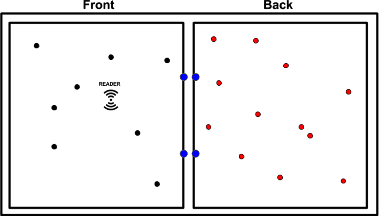
Schematic representation of the scenario.

4 Proposed approaches

An overview of the proposed approaches is provided in this section.

4.1 Heuristic approach

The first proposed model is a simple heuristic approach. The proposed heuristic uses the reference tags as a sort of reference point. Since the reference tags are placed on the partition wall between the room where the reader is (i.e., front) and the back shop (i.e., back), the heuristic compares the Read Rate (RR) of each tag with the average RR of the reference tags: when the RR of the considered tag is lower than the RR of the reference ones, the tag is assumed to be in the back, otherwise it is considered in the front.

4.2 Logistic regression

The logistic regression is the same model we already implemented in our previous work. The input of the logistic regression, as described in Esposito et al. (2021), is a vector of 7 elements: (i) the RR of the tag (i.e., how many times it has been read), (ii) its average RSSI, (iii) the median of its RSSI, and other four quantiles (respectively 5%, 25%, 75%, and 95%).

4.3 Logistic Regression with reference tags

This model is very similar to the previously described one, although it tries to take advantage of the reference tags. Each time a reading is carried out and the model must define which tags are in the front and which in the back, it is provided with not just the information concerning the tag to be localised, but also the information concerning the reference tags. Hence, given for example the global number of reference tags, g, the input of the model is a vector of 7 + 7g elements, where the first 7 values are the same inputs of the previously described model (respectively the RR of the tag to classify, its average RSSI, its median RSSI, and the 5%, 25%, 75%, 95% quantiles of its RSSI), while the remaining 7g values are the same parameters for all the g reference tags.

4.4 Neural Network

The next implemented and tested model is a deep neural network. In order to avoid complicated parameters tuning we implemented one of the most widespread configurations with three hidden layers of 32 nodes each. The size of the input layer is the same of the logistic regression with reference tags (i.e., 7 + 7g where g is again the global number of reference tags) and in this case it was therefore of 35 nodes. Finally, the output layer is made of a single node with the sigmoid activation function.

All the nodes of the network (except for the output node) use a classic ReLU activation function, and the training is made using the Adam algorithm (Jais et al., 2019) and batches of 1024 rows. During the training a slight dropout regularisation technique (Srivastava, 2013) is used in all three layers to avoid overfitting.

A representation of the implemented neural network is reported in Fig. 2.

Fig. 2

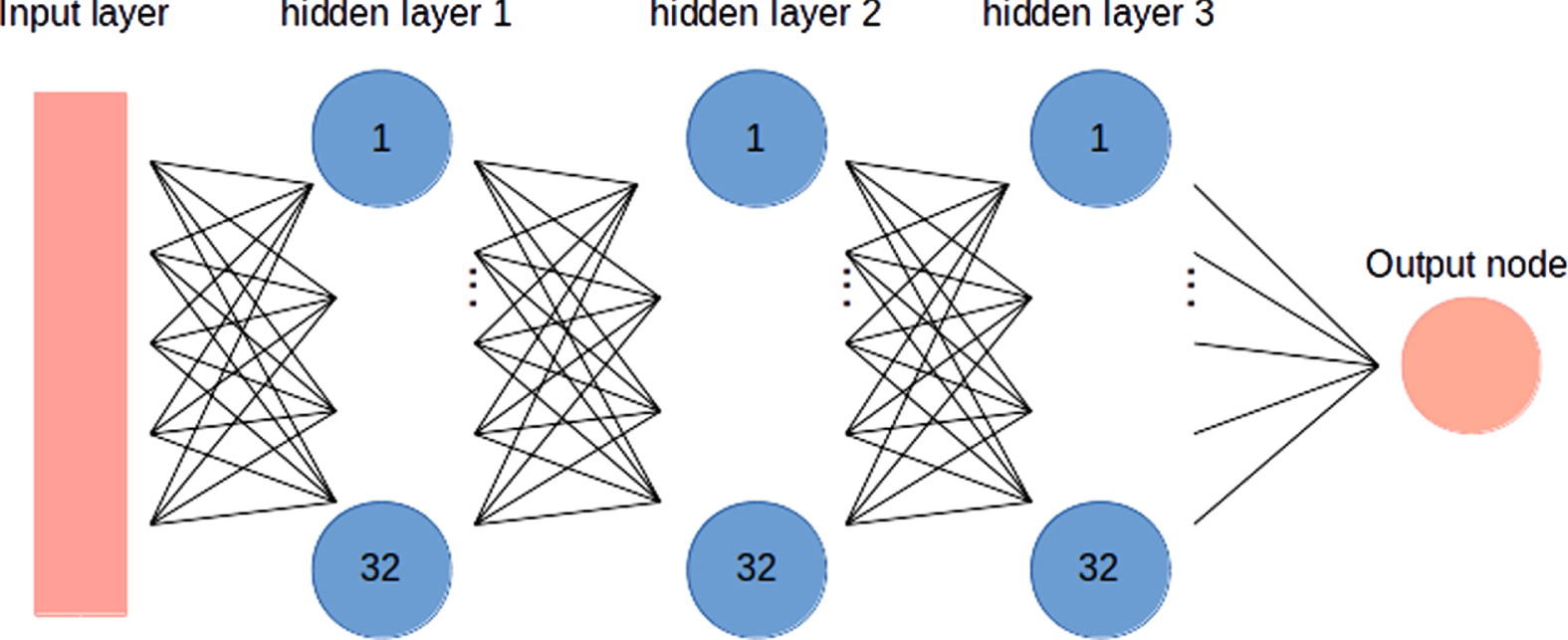
Implemented neural network.

4.5 Convolutional Neural Network

In the last model, the concept of time is also considered. Since the readings are essentially made by an operator who walks around the shop for the entire duration of the reading session (∼60 seconds), it might happen that, given a tag to classify, some readings result having a very high value of RSSI (because the operator is close to the tag) and others result having a very low value of RSSI (because the operator is on the opposite side of the area). This behaviour might be confusing for a model that does not consider the instant of time in which the readings take place and therefore deteriorate the classification accuracy.

Given a tag to be classified, using a Convolutional Neural Network (CNN) offers the possibility to split the readings depending on the time in which they took place and provide them separately to the model. More precisely, the input of our CNN is a T x (7 + 7g) matrix where g is again the number of reference tags, and T is the number of time windows in which the reading session has been split. If a reading session lasts 60 seconds and the number of time windows considered is T = 3, the first line of the input matrix contains the monitored parameters (i.e., RR, average RSSI, median RSSI, 5%, 25%, 75%, 95% RSSI) relative to the tag to classify and the reference tags with respect to the first 20 seconds of the reading session, the second line contains the same information with respect to the readings occurred between 20 and 40 seconds from the reading session’s beginning, and, similarly, the third line contains the same information with respect to the last 20 seconds of the reading session. In this way, the model has information relative to the tag to be classified in T different instant of time, and not just a single view of the whole reading session (see Fig. 3).

Fig. 3

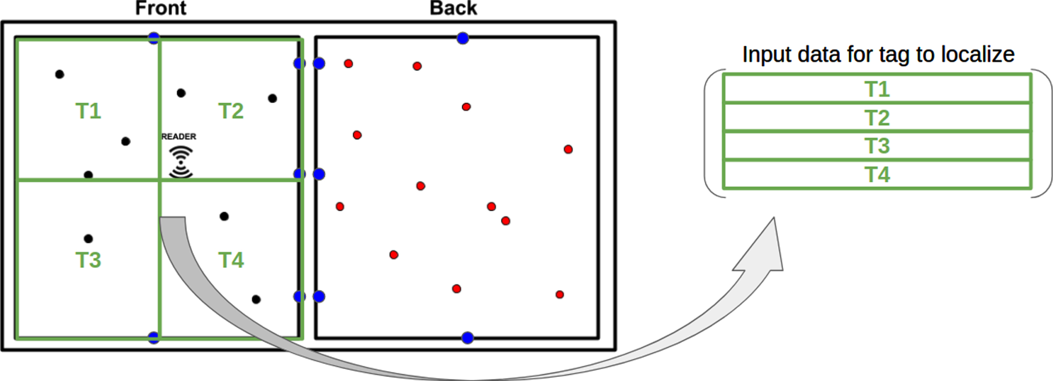
Representation of the time windows concept.

Concerning the architecture of the CNN, we used a common topology mostly used with the MNIST dataset, made of the following elements:

An input layer T x (7 + 7g) x 1 where T = 3 and g = 4.

A 2D convolution layer with 32 output filters and a 3×3 kernel.

A max pooling layer of size 2×2.

A 2D convolution layer with 64 output filters and a 3×3 kernel.

A max pooling layer of size 2×2.

A 2D convolution layer with 128 output filters and a 3×3 kernel.

A max pooling layer of size 2×2.

A flattener.

A dense layer of 128 nodes.

An output node with the sigmoid activation function.

All the nodes (except for the output node) make use of the LeakyReLU activation function, the Adam algorithm (Jais et al., 2019) is used for training, and a dropout regularisation (Srivastava, 2013) is used for the dense layer in order to prevent overfitting. The choice of the LeakyReLU depends on fact that the available dataset was too small to provide a correct training of a CNN, and, as proved by Dubey & Jain (2019), the LeakyReLU results very efficient in cases characterised by sparse gradient (due to a not big enough dataset).

The architecture of the implemented convolutional neural network is shown in Fig. 4.

Fig. 4

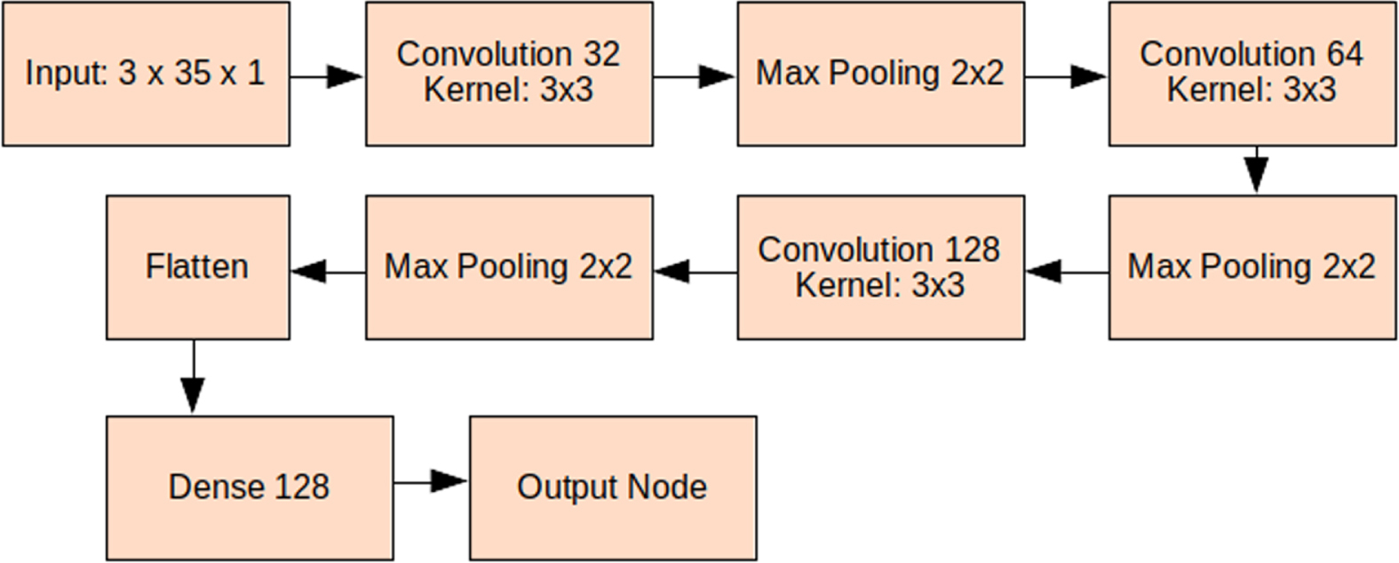
Implemented convolutional neural network.

5 Experiments and validation

Tables 2 to 6 report respectively the results obtained by the above-described models in the 24 different scenarios.

Table 2
Results of the logistic regression without reference tags

Scenario Accuracy Precision Front Recall Front Precision Back Recall Back

1 0.832 1.000 0.773 0.635 1.000

2 0.949 1.000 0.934 0.837 1.000

3 1.000 1.000 1.000 1.000 1.000

4 0.918 1.000 0.904 0.709 1.000

5 0.987 0.983 0.994 0.993 0.980

6 0.984 0.983 0.988 0.986 0.980

7 0.993 1.000 0.988 0.987 1.000

8 0.979 0.965 1.000 1.000 0.950

9 0.356 0.988 0.304 0.112 0.987

10 0.431 0.995 0.329 0.212 0.991

11 0.257 0.952 0.097 0.191 0.990

12 0.207 1.000 0.091 0.138 1.000

13 0.570 0.986 0.365 0.412 0.990

14 0.514 0.998 0.273 0.406 0.998

15 0.447 1.000 0.154 0.384 1.000

16 0.361 1.000 0.116 0.302 1.000

17 0.358 0.933 0.166 0.266 0.974

18 0.101 1.000 0.071 0.037 1.000

19 0.103 1.000 0.071 0.037 1.000

20 0.529 0.966 0.500 0.143 0.866

21 0.692 1.000 0.440 0.600 1.000

22 0.671 0.968 0.547 0.483 0.957

23 0.507 1.000 0.309 0.359 1.000

24 0.824 0.992 0.755 0.636 0.987

Scenario	Accuracy	Precision Front	Recall Front	Precision Back	Recall Back
1	0.832	1.000	0.773	0.635	1.000
2	0.949	1.000	0.934	0.837	1.000
3	1.000	1.000	1.000	1.000	1.000
4	0.918	1.000	0.904	0.709	1.000
5	0.987	0.983	0.994	0.993	0.980
6	0.984	0.983	0.988	0.986	0.980
7	0.993	1.000	0.988	0.987	1.000
8	0.979	0.965	1.000	1.000	0.950
9	0.356	0.988	0.304	0.112	0.987
10	0.431	0.995	0.329	0.212	0.991
11	0.257	0.952	0.097	0.191	0.990
12	0.207	1.000	0.091	0.138	1.000
13	0.570	0.986	0.365	0.412	0.990
14	0.514	0.998	0.273	0.406	0.998
15	0.447	1.000	0.154	0.384	1.000
16	0.361	1.000	0.116	0.302	1.000
17	0.358	0.933	0.166	0.266	0.974
18	0.101	1.000	0.071	0.037	1.000
19	0.103	1.000	0.071	0.037	1.000
20	0.529	0.966	0.500	0.143	0.866
21	0.692	1.000	0.440	0.600	1.000
22	0.671	0.968	0.547	0.483	0.957
23	0.507	1.000	0.309	0.359	1.000
24	0.824	0.992	0.755	0.636	0.987

Table 3

Results of the logistic regression without reference tags

Scenario	Accuracy	Precision Front	Recall Front	Precision Back	Recall Back
1	1.000	1.000	1.000	1.000	1.000
2	0.995	0.994	1.000	1.000	0.976
3	1.000	1.000	1.000	1.000	1.000
4	0.990	0.994	0.994	0.972	0.986
5	0.987	0.983	0.994	0.993	0.980
6	0.990	0.994	0.988	0.985	0.993
7	1.000	1.000	1.000	1.000	1.000
8	0.996	0.994	1.000	1.000	0.993
9	0.964	0.992	0.968	0.666	0.967
10	0.979	0.996	0.980	0.896	0.981
11	0.975	0.994	0.974	0.895	0.977
12	0.926	0.988	0.926	0.665	0.928
13	0.942	0.971	0.944	0.870	0.950
14	0.975	0.988	0.974	0.949	0.976
15	0.973	0.985	0.972	0.949	0.974
16	0.969	0.985	0.971	0.928	0.962
17	0.834	0.937	0.845	0.636	0.827
18	0.945	0.992	0.950	0.466	0.933
19	0.965	0.988	0.976	0.333	0.666
20	0.973	0.993	0.978	0.853	0.900
21	0.954	0.960	0.958	0.952	0.948
22	0.983	0.994	0.982	0.960	0.988
23	0.936	0.978	0.934	0.860	0.959
24	0.930	0.962	0.934	0.867	0.920

Table 4

Results of the logistic regression with reference tags

Scenario	Accuracy	Precision Front	Recall Front	Precision Back	Recall Back
1	0.996	1.000	0.994	0.988	1.000
2	0.972	0.988	0.976	0.952	0.948
3	1.000	1.000	1.000	1.000	1.000
4	0.995	0.994	1.000	1.000	0.972
5	0.996	1.000	0.994	0.993	1.000
6	0.990	0.994	0.988	0.986	0.993
7	1.000	1.000	1.000	1.000	1.000
8	1.000	1.000	1.000	1.000	1.000
9	0.977	0.997	0.976	0.819	0.990
10	0.976	0.995	0.977	0.889	0.976
11	0.970	0.988	0.975	0.898	0.946
12	0.900	0.991	0.893	0.601	0.944
13	0.920	0.975	0.902	0.958	0.950
14	0.973	0.987	0.972	0.947	0.974
15	0.965	0.981	0.966	0.937	0.965
16	0.970	0.984	0.974	0.935	0.960
17	0.864	0.950	0.869	0.941	0.809
18	0.938	0.986	0.950	0.383	0.733
19	0.804	0.988	0.809	0.133	0.666
20	0.973	0.993	0.978	0.900	0.900
21	0.947	0.969	0.934	0.928	0.963
22	0.894	1.000	0.851	0.859	1.000
23	0.961	0.987	0.952	0.926	0.977
24	0.921	0.969	0.916	0.850	0.934

Table 5

Results of the neural network

Scenario	Accuracy	Precision Front	Recall Front	Precision Back	Recall Back
1	0.973	1.000	0.964	0.946	1.000
2	0.929	0.949	0.970	0.761	0.757
3	0.970	0.970	1.000	0.833	0.833
4	0.990	0.988	1.000	1.000	0.958
5	0.990	0.994	0.988	0.986	0.993
6	0.983	0.988	0.982	0.978	0.986
7	1.000	1.000	1.000	1.000	1.000
8	0.982	0.971	1.000	1.000	0.959
9	0.983	0.993	0.986	0.900	0.949
10	0.917	0.991	0.910	0.727	0.957
11	0.927	0.955	0.961	0.715	0.750
12	0.805	0.952	0.830	0.469	0.674
13	0.899	0.926	0.939	0.876	0.840
14	0.954	0.970	0.962	0.926	0.940
15	0.936	0.934	0.975	0.954	0.861
16	0.925	0.956	0.941	0.862	0.886
17	0.732	0.797	0.904	0.128	0.238
18	0.959	0.972	0.985	0.233	0.333
19	0.977	0.977	1.000	0.333	0.333
20	0.792	0.965	0.807	0.502	0.566
21	0.882	0.925	0.857	0.546	0.546
22	0.894	0.939	0.916	0.916	0.831
23	0.831	0.925	0.845	0.505	0.644
24	0.904	0.956	0.904	0.806	0.907

Table 6

Results of the convolutional neural network

Scenario	Accuracy	Precision Front	Recall Front	Precision Back	Recall Back
1	0.987	1.000	0.982	0.923	1.000
2	0.980	0.988	0.988	146.6	0.952
3	0.994	0.994	1.000	1.000	0.916
4	0.990	0.988	1.000	1.000	0.958
5	0.993	0.994	0.994	0.993	0.993
6	0.996	0.994	1.000	1.000	0.993
7	1.000	1.000	1.000	1.000	1.000
8	0.989	1.000	0.982	0.977	1.000
9	0.981	0.980	0.996	0.975	0.921
10	0.848	0.997	0.819	0.807	0.987
11	0.968	0.973	0.991	0.955	0.872
12	0.971	0.974	0.992	0.8163	0.827
13	0.956	0.959	0.972	0.943	0.933
14	0.961	0.976	0.965	0.936	0.954
15	0.963	0.976	0.968	0.945	0.956
16	0.963	0.974	0.975	0.944	0.933
17	0.992	0.991	1.000	1.000	0.219
18	0.971	0.988	0.973	0.628	0.666
19	0.931	0.931	1.000	0.000	0.000
20	1.000	1.000	1.000	1.000	1.000
21	1.000	1.000	1.000	1.000	1.000
22	0.966	0.976	0.976	0.949	0.943
23	0.851	0.814	0.863	0.718	0.877
24	0.966	0.972	0.982	0.956	0.931

As it is visible from the tables, and represented in Fig. 5, all the proposed models are very accurate except for the heuristic approach. More in detail, looking at Table 2, we can see how the heuristic approach has a good accuracy (∼95%) in the first scenarios characterised by a low density of hanging clothes, but quickly deteriorate in more complex scenarios where the density of tags increases and the disposition of clothes changes.

Fig. 5

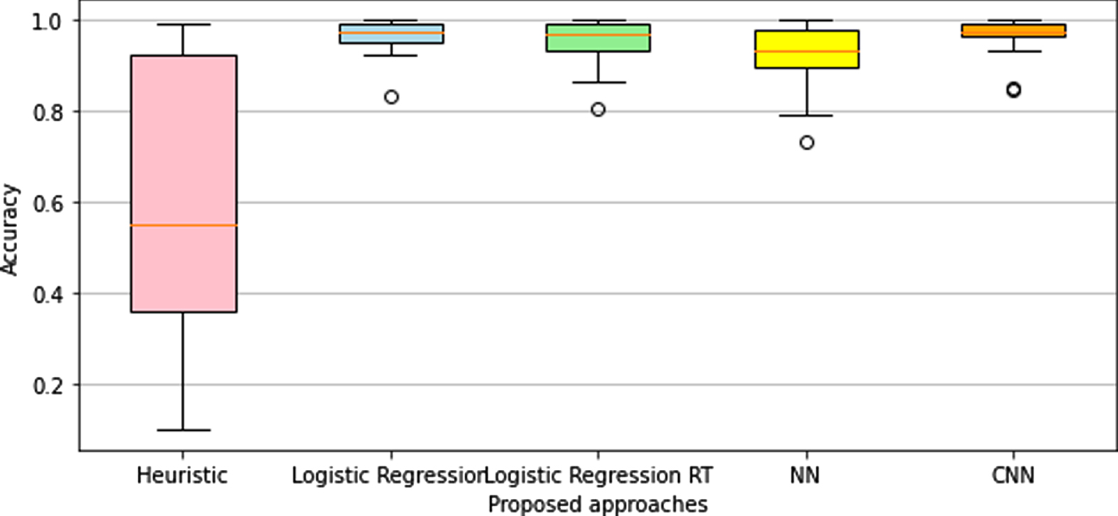
Comparison of the proposed models.

The comparison between other models is clearer in Fig. 6. All the models represented in Fig. 6 are surprisingly accurate, however, the logistic regression with reference tags and the NN are less accurate than the simple logistic regression that we also proposed in our previous work. As this might seem strange, a possible justification could be the, probably unsupportive, presence of reference tags. Indeed, reference tags could be a negative reference point when the operator is moving in the front area, introducing some noise that could deteriorate the model’s efficiency.

Fig. 6

Comparison of proposed models except for the heuristic.

As it clearly emerges from Figs. 5 and 6 , the best results are achieved by the CNN approach. This approach, in fact, outperforms the others in terms of accuracy. This could be justified by the introduction of the time variable, which also explains why the use of reference tags alone, i.e., without an implicit information concerning the position of the operator in the specific time window, cannot help the model to better localize the tags.

For sake of clarity, and in order to provide a more extensive analysis of the surrounding conditions, an analysis of variance (ANOVA) has been performed on the accuracy of the most performant approach (i.e., CNN). These results are presented in Table 7. The p-values of the ANOVE show that the disposition of tags and their density, as already guessed by the JSD values (see Table 1), are the aspect with the greatest impact on the model accuracy. The wall type also has a considerable impact, but it is still not comparable to the above-mentioned disposition of tags. The combination of wall type and disposition is also a relevant aspect, which is however accentuated again by the great effect of the tags disposition. Moreover, a comparison of Tables 1 and 7 provides very interesting information. It is clear that the choice of a classification model over another is a non-negligible aspect for a correct implementation of SBS (see Fig. 5 and 6). However, there is a great correlation between the deterioration of the CNN’s accuracy (Table 6) and the JSD values presented in Table 1. The lowest accuracy of the CNN is obtained in scenarios 10, 19 and 23, which are among those with the lowest JSD value (and therefore the least sharp distinction between tags in terms of read rate). We can conclude that, for a correct and efficient implementation of the SBS, the key aspects are (i) the classification model and (ii) the way in which items are stored and placed inside the retail shop. None of these two aspects should be neglected or prevail over the other.

Table 7

ANOVA to explore the effect of the environmental aspects on the CNN

Source	SS	DF	MS	F	p-value
Power	8.1753326e-05	1.0	8.1753326e-05	0.015027030	0.90265174
Wall	0.028304476	3.0	0.009434825	1.734209652	0.16394858
Disposition	0.041377175	2.0	0.020688587	3.802756983	0.02519070
Power ^* Wall	0.021743701	3.0	0.007247900	1.332232273	0.26742616
Power ^* Disposition	0.012215785	2.0	0.006107892	1.122688115	0.32897458
Wall ^* Disposition	0.077897464	6.0	0.012982910	2.386381100	0.03291425
Power ^* Wall ^* Disposition	0.024671108	6.0	0.004111851	0.7557969	0.60611003
Residual	0.620207655	114.0	0.0054404

6 Conclusions

In this paper, the recent RFID software-based shielding solution proposed by G. Esposito, Mezzogori, Neroni, Rizzi, and Romagnoli (2021) is further investigated. The solution, based on item-level tags and particularly suitable for the fashion and apparel sector, provides greater flexibility, and it could be linked to economic savings, as it can work without a physical shielding between different store areas. In the present study, SBS has been tested with (i) different software approaches of increasing complexity; (ii) different wall types and thickness, as well as with (iii) varying tags dispositions and densities. Also, in the present work, reference tags have been introduced, to support the classification model.

Firstly, the impact of wall type and thickness, and of tags dispositions and densities is non negligible. By using the Jensen-Shannon divergence (JSD) between the read rate of tags in the front and that of tags in the back, JSD values show three main clusters corresponding to three different classification difficulties: namely, low density hanging tags can be classified quite easily between the front and the back, regardless of reading power and partition wall type and thickness, as their average JSD is ∼0.8 (scenarios 1–8 in Table 1). If we increase the density of hanging garments, the classification becomes more difficult (scenarios 9–16 in Table 1, average JSD ∼0.56). Similarly, folded garments present a complex classification even at low density, with an average JSD of ∼0.62 and the greatest JSD variability (scenarios 17–24 in Table 1).

In these conditions, 5 different software approaches were used for the proposed classification problem, ranging from a naive heuristic approach, to a Convolutional Neural Network. All these approaches have been evaluated in each of the 24 scenarios in terms of precision and recall, both in the front and in the back, and summarized with a global accuracy value. It emerges that a simple approach can be effective with low density of hanging tags, with a global accuracy ranging from 83% to over 99%. The accuracy of this simple model, however, is completely inadequate with higher tags density or folded garments. The logistic regression without reference tags, as already introduced in previous research, is both effective and robust, with an average accuracy value of 96,6% and just one outlier scenario of accuracy below 90% (scenario 17).

Quite surprisingly, the addition of reference tags to the logistic regression model, as well as the use of reference tags in a NN, do not improve average accuracy. Both these approaches, in fact, underperform against the logistic regression approach. The only model that is capable of improving the results of the logistic regression is the CNN presented in Section 4.5. Indeed, the use of time windows improves the overall performance, by providing a slightly higher average accuracy (96,7%), and also an improvement in the median of accuracy (97,6%, against 97,4% median accuracy of the logistic regression). We note that these results have been achieved by the CNN with two outlier scenarios with an approximate accuracy of 85%, namely scenario 10 and 23. Thus, the CNN with time windows proves to be a promising field of research for improving SBS.

As per the impact of surrounding conditions, we note that the ANOVA we performed on the CNN accuracy only reports Disposition (i.e., tags disposition and density) as a significant factor at common levels (i.e., p value of 0.025). The second-most significant factor is Wall (i.e., wall type and thickness), with a p value of 0.164, while the power level is insignificant. This is also proved by the fact that the combined factors Disposition ^* Wall are also significant (p value around 0.033). We can therefore conclude that tags disposition and density play a key role in the SBS accuracy results calculated via the CNN approach, that is the most performing one.

Future research lines might involve the following points: (i) testing SBS in different conditions, possibly close to the store-like conditions (i.e., real store environment, with tags disposition and density of business applications); (ii) improving the SBS approaches, with a particular focus on the CNN, which proved capable of delivering promising results, and on different time windows; (iii) further investigate on how reference tags could be used in the most supportive way; (iv) extend the tests to different handheld readers, which could also provide more reading data (e.g., phase), and therefore different results. Indeed, the authors are already at work on some of these points for future studies.

References

Abugabah,

, Nizamuddin,

, Abuqabbeh,

(2020) A review of challenges and barriers implementing RFID technology in the Healthcare sector. Procedia Computer Science 170, 1003–1010. https://doi.org/10.1016/j.procs.2020.03.094

Bertolini,

, Rizzi,

, Romagnoli,

, Volpi,

(2017) Testing an RFID receiving gate for improving process accuracy in fashion and apparel retail. RTSI 2017 - IEEE 3rd International Forum on Research and Technologies for Society and Industry, Conference Proceedings, i. https://doi.org/10.1109/RTSI.2017.8065916

Bertolini,

, Romagnoli,

, Weinhard,

(2017) Proposing aValue-Added Indicators framework for the apparel and fashion sector: Design and empirical evaluation. International Journal of RF Technologies: Research and Applications 8((3)), 143–164. https://doi.org/10.3233/RFT-171674

Buffi,

, Nepa,

, Lombardini,

(2014) A phase-based technique for localization of UHF-RFID tags moving on a conveyor belt: Performance analysis and test-case measurements, IEEE Sensors Journal 15(1), 387–396.

Cilloni,

, Leporati,

, Rizzi,

, Romagnoli,

(2019) State of the art of item-level RFID deployments in fashion and apparel retail. International Journal of RF Technologies 10((3–4)), 65–88. https://doi.org/10.3233/RFT-190174

Dubey,

A. K

, Jain,

(2019) Study of Convolution Neural Network’s Relu and Leaky-Relu Activation Functions. In Applications of Computing, Automation and Wireless Systems in Electrical Engineering (pp. 873–880). https://doi.org/10.1007/978-981-13-6772-4 76.

Esposito,

, Romagnoli,

, Sandri,

, Villani,

(2015) Deploying RFID in the fashion and apparel: sector an “ in the field ” analysis to understand where the technology is going to, XX Summer School “Francesco Turco” in Industrial Mechanical Plants.

Esposito,

, Mezzogori,

, Neroni,

, Rizzi,

, Romagnoli,

(2021) Software-based shielding for real-time inventory count in different store areas: A feasibility analysis in fashion retail. International Journal of RF Technologies: Research and Applications, International Journal of RF Technologies: Research and Applications 12(1), 53–68. https://doi.org/10.3233/RFT-210294

Esposito,

, Mezzogori,

, Neroni,

, Rizzi,

, Romagnoli,

, Rosa,

(2021) A review of RFID based solutions for indoor localization and location-based classification of tags. In press, Proceedings of the Summer School Francesco Turco.

10.

Farid,

, Nordin,

, Ismail,

(2013) Recent advances in wireless indoor localization techniques and sys442 tem. Journal of Computer Networks and Communications, 2013. https://doi.org/10.1155/2013/185138

11.

Goyal,

, Hardgrave,

B. C

, Aloysius,

J. A

, Dehoratius,

(2016) The effectiveness of RFID in backroom and sales floor inventory management. The International Journal of Logistics Management 27(3), 795–815. https://doi.org/10.1108/IJLM-03-2015-0051

12.

Hardgrave,

B. C.

(2012) Omnichannel retailing - You can’t do it without RFID. RFID Journal. http://www.rfidjournal.com/articles/view?10247.

13.

House,

, Connell,

, Milligan,

, Austin,

, Hayes,

T. L

, Chiang,

(2011) Indoor localization using pedestrian dead reckoning updated with RFID-based fiducials. 2011 Annual International Conference of the IEEE Engineering in Medicine and Biology Society, 7598–7601..

14.

Hu,

, Cheng,

, Zhang,

(2011) A Zigbee-based localization algorithm for indoor environments, Proceedings of International Conference on Computer Science and Network Technology 3, 1776–1781.

15.

Jais,

I. K. M

, Ismail,

A. R

, Nisa,

S. Q.

(2019) Adam Optimization Algorithm for Wide and Deep Neural Network. Knowledge Engineering and Data Science 2(1), 41. https://doi.org/10.17977/um018v2i12019p41-46

16.

Japanese Ministry of Economy Trade and Industry. (2017). Declaration of Plan to Introduce 100 Billion Electronic Tags for Products in Convenience Stores Formulated. News Releases. https://www.meti.go.jp/english/press/2017/0418003.html.

17.

Knapp,

, Romagnoli,

(2021) RFID systems optimisation through the use of a new 459 RFID network planning algorithm to support the design of receiving gates. Journal of Intelligent Manufacturing https://doi.org/10.1007/s10845-021-01858-0

18.

Li,

, Mo,

, Zhang,

(2019) Review on UHF RFID Localization Methods. IEEE Journal of Radio Frequency Identification 3(4), 205–215. https://doi.org/10.1109/JRFID.2019.2924346

19.

Liu,

, Darabi,

, Banerjee,

, Liu,

(2007) Survey of wireless indoor positioning techniques and systems, IEEE Transactions on Systems, Man, and Cybernetics, Part C (Applications and Reviews) 37(6), 1067–1080.

20.

Menéndez,

M. L

, Pardo,

J. A

, Pardo,

M. C.

(1997) The Jensen-Shannon divergence. Journal of the Franklin Institute 334(2), 307–318. https://doi.org/10.1016/S0016-0032(96)00063-4

21.

Metzger,

, Thiesse,

, Gershwin,

, Fleisch,

(2013) The impact of false-negative reads on the performance of RFID-based shelf inventory control policies. Computers and Operations Research 40(7), 1864–1873. https://doi.org/10.1016/j.cor.2013.02.001

22.

Pai,

, Sasi,

, Mantripragada,

P. S

, Malpani,

, Aggarwal,

(2012). Padati: A robust pedestrian dead reckoning system on smartphones. 2012 IEEE 11th International Conference on Trust, Security and Privacy in Computing and Communications, 2000–2007.

23.

Rizzi,

, Romagnoli,

(2017) Testing and deploying an RFID-based Real-Time Locating System at a fashion retailer: A case study. In R. Rinaldi & R. Bandinelli (Eds.), Business Models and ICT Technologies for the Fashion Supply Chain (Vol. 413, pp. 201–214). Springer International Publishing. https://doi.org/10.1007/978-3-319-48511-9

24.

Seco,

, Jiménez,

A. R

, Prieto,

, Roa,

, Koutsou,

(2009). A survey of mathematical methods for indoor localization. 2009 IEEE International Symposium on Intelligent Signal Processing, 9–14.

25.

Solti,

, Raffel,

, Romagnoli,

, Mendling,

(2018) Misplaced product detection using sensor data without planograms. Decision Support Systems 112, 76–87. https://doi.org/10.1016/j.dss.2018.06.006

26.

Srivastava,

(2013). Improving neural networks with dropout. University of Toronto..

27.

Swedberg,

(2019). Fashion Retailer Leverages Virtual Shielding to Overcome Stray RFID Reads. RFID Journal.

28.

Uckelmann,

, Romagnoli,

(2016). RF-based Locating of Mobile Objects. 6th International Conference on the Internet of Things (IoT‘16), 147–154.

29.

Vivaldi,

, Melai,

, Bonini,

, Poma,

, Salvo,

, Kirchhain,

, Tintori,

, Bigongiari,

, Bertuccelli,

, Isola,

, Di Francesco

(2020) Atemperature-sensitive RFID tag for the identification of cold chain failures. Sensors and Actuators A: Physical 313, 112182. https://doi.org/10.1016/j.sna.2020.112182

30.

Vossiek,

, Wiebking,

, Gulden,

, Weighardt,

, Hoffmann,

(2003). Wireless local positioning concepts, solutions, applications. Radio and Wireless Conference, 2003. RAWCON’03. Proceedings, 219–224.

31.

Wu,

, Tao,

, Gong,

, Yin,

, Ding,

(2019) A Fast UHF RFID Localization Method Using Unwrapped Phase-Position Model. IEEE Transactions on Automation Science and Engineering 16(4), 1698–1707. https://doi.org/10.1109/TASE.2019.2895104

32.

Xu,

, Wu,

, Li,

, Zhu,

, Wang,

(2018) An RFID indoor positioning algorithm based on support vector regression, Sensors 18(5), 1504.

33.

Yao,

C.-Y

, Hsia,

W.-C.

(2018) An Indoor Positioning System Based on the Dual-Channel Passive RFID Technology. IEEE Sensors Journal 18(11), 4654–4663. https://doi.org/10.1109/JSEN.2018.2828044

34.

Yunhao,

, Zheng,

(2011) Location, Localization, and Localizability: Location-awareness Technology for Wireless Networks, Springer Publications 3(4).