A new statistical methodology for assessing mechanical survivability of brittle materials

Abstract

Brittle materials such as ceramics are subject to fracture without warning. Because non-destructive techniques are unreliable for determining potential fracture sources in ceramic materials one must rely on statistical analysis of laboratory strength data. This data is used to determine the minimum strength, and its uncertainty, of a set of specimens, and then must translate this laboratory data into a projection of the reliability of components manufactured from the material. This paper sets forth new guidelines for the choice of a statistical methodology to fit the laboratory data and puts forth a procedure – known as tolerance limits and coverage – to extrapolate this data to predict component reliability. Data on a borosilicate glass is used to demonstrate the usefulness of this procedure.

Keywords

Aluminum oxide ASTM C1239-07 brittle fracture ceramics glass silicon nitride statistical analysis statistics strength survivability tolerance limits uncertainty quantification Weibull distribution

1. Introduction

The seemingly unpredictable nature of fracture in brittle materials, e.g., ceramics, semiconductors, or brittle metal alloys, complicates the job of the engineer in designing and manufacturing parts that will not fail in service. All brittle materials contain a distribution of “flaws” that can lead to failure. By “flaws” we do not mean that there were necessarily defects in production, although processing flaws that are intersected by the tensile surface can also act as failure sources. Small surface cracks are created as a natural result of cutting and grinding. These cracks vary in size, shape, and orientation and frequently serve as the sources of failure. Tensile stresses on this flaw population arise, not just due to externally applied mechanical loads, but also due to processing-induced stresses, thermal gradients, phase transformations, or the presence of applied electric fields.

The most important parameter in any prediction of survivability is the minimum stress which could lead to the fracture of a part in service, and knowledge of the uncertainty in this stress. Knowledge of survivability requires that we have a method to guarantee that the most severe flaw in a component is not subjected to such a stress.

Three methods for assuring the reliability of brittle materials are potentially available. The most direct approach would be a non-destructive evaluation of a part prior to it being placed into service, which in principle would allow the identification of a flaw that could lead to failure. Unfortunately, no non-destructive procedures are available with the necessary sensitivity to distinguish the one critical flaw from the many other small cracks.

A second method is proof testing in which a part is loaded to a stress exceeding that expected in service, and then rapidly unloaded [7]. While this procedure can be effective if carried out correctly, it is expensive to conduct on every part, and a significant loss of parts during the proof test should be expected. In addition, the proof-test stress must be conducted in a special environment, and stresses must be applied under the same loading condition as that the part will experience in service.

One is therefore left with the necessity of using the statistical fracture behavior of the material as the measure of flaw severity. It is crucial to know not just the minimum stress at which failure could occur, but also to what degree of confidence it can be specified. Since only a relatively small subset of the entire population of manufactured parts is tested, it is important to have methods by which one can use laboratory data to predict failure stresses in the entire expanse of all parts.

Two-parameter Weibull statistics is at present the primary method by which strength distributions are fit and analyzed, and is the method advocated in ASTM standards [3,4] to describe strength distributions for brittle materials. The choice of the Weibull function as the standard methodology was primarily due to the opinion that this expression represents the physics of the process, namely that there exists a “weak link” which, if broken, leads to failure [18,19]. The two-parameter Weibull distribution which allows for failure at stresses approaching zero (Eq. (1)), is used today, in-part because of the convergence issues involved in estimating the parameters for a three-parameter Weibull distribution for small values of the shape parameter. $\begin{eqnarray}P_{f}=1-\exp \left[-\left(\frac{S}{S_{0}}\right)^{M}\right].\end{eqnarray}$ (1) P _f is the probability of failure; S is the stress at fracture; S ₀ is known as the scale parameter (also known as the Weibull characteristic strength in materials science literature), and M is the shape parameter (m2 will be used when referring to the shape parameter for a two-parameter Weibull). The shape parameter is also named Weibull modulus even though it is dimensionless. It is our contention that the use of a two-parameter Weibull distribution is unduly conservative; large flaws that would grow at extremely small stresses could be visually observed, or possibly the component would break before being placed into service; in addition, this function is not necessarily the best fit to the test data. The Weibull functions are only one of many possible expressions that could be employed. However, there is no evidence to support that, a-priori, the Weibull function is superior to others.

This paper provides a different statistical analysis technique which allows one to determine the minimum strength of brittle parts, including a discussion of the methods by which the results of laboratory-scale specimens can be used to predict the reliability of large numbers of parts. The methodology is demonstrated for a number of materials [6,11].

2. Measurement and analysis procedures

The most important experimental parameter that must be determined to assure the survival of a part is the minimum strength in the distribution of manufactured parts. This minimum strength provides a measure of the most severe flaw existing in the as-produced material. Severity is determined by both flaw size and shape, a key assumption being that no flaws more severe than that leading to the minimum initial strength are introduced during service. It would be advantageous if the strength distribution of actual parts could be obtained under in-service loading conditions. However, this can be difficult and costly. Consequently, tests are usually conducted on small pieces of the same material. The processing procedures and surface treatments, e.g., machining and polishing, of these specimens must be identical to that seen by the component.

Because of the propensity of brittle materials to fail from surface flaws, flexural tests, conducted in either uniaxial or biaxial loading, are suitable and the easiest methods of measuring fracture strength. The decision of whether to conduct uniaxial or biaxial tests is based on a number of factors, e.g., the form of the material (plates, bars, etc.), whether edges in the part will be subject to significant stresses. Details of recommended testing procedures are given in the studies by Freiman and Mecholsky [10] and Quinn and Morrell [17]. It is usually recommended that a minimum of thirty specimens be tested to assure that an adequate statistical distribution can be established [12]. However, the actual number of specimens that one should test will depend on the scatter in the data and the confidence level desired. If uniaxial flexural specimens are cut from a plate, one must make sure to randomize them with respect to the machining direction, since strengths perpendicular and parallel to the direction of grinding are different [13]. If a component could possibly experience a stress state that could cause it to fail from internal flaws that are not intersected by the surface, e.g., pores or inclusions, flexural tests will not be effective, and direct tensile tests will be required.

One of the important factors is that the flaws that cause failure in the test specimens are the same as those in the components. In the simplest case, all flaws leading to failure are of the same type, and come from one population, i.e., one source. In some instances, however, there are multiple flaw populations involved leading to more complex strength distributions. The presence of multiple flaw distributions usually manifests itself as a segmented strength-distribution plot. Fractographic analysis of the broken specimens, particularly those in the low-strength region, is important to determine the actual cause of failure, and to separate unusually low strengths from those in the general population [16].

3. A 4-step methodology

We present a four-step approach to the calculation of the probability of failure of a given component. All of the calculations in this procedure make use of the program, “Dataplot” [8].

Step 1: Pick a function with which to fit the strength distribution of the set of specimens.

A somewhat obvious first choice is the three-parameter Weibull function. The three-parameter Weibull distribution differs from the two-parameter function in the introduction of a third parameter called the location parameter, S _m, which is also known as the minimum lower strength. For the 3-parameter Weibull function the shape parameter, M, will be referred to as m3 to distinguish it from the shape parameter for the 2-parameter Weibull function. $\begin{eqnarray}P_{f}=1-\exp \left[-\left(\frac{S-S_{m}}{S_{0}}\right)^{M}\right].\end{eqnarray}$ (2) In a recent paper [9] five expressions were compared as fits to the borosilicate (BK 7) glass data (two-parameter Weibull, three-parameter Weibull, normal, two-parameter lognormal, and three-parameter lognormal). There are large numbers of other possible functions that can be used to fit the data. For the purpose of this demonstration paper, we choose to limit our choice to just three, namely: (1) normal, (2) 2-parameter Weibull, and (3) 3-parameter Weibull.

Step 2: Choose a method to fit the function to the data, i.e., an estimation method. We choose the Maximum Likelihood Estimation (MLE) (see, e.g., Bury [5, p. 161–168], Aldrich [1], Anderson [2]), which is the most common method currently in use to fit strength distributions for brittle materials [3].

Step 3: The choice of a function to fit a data set should be based on the Goodness-of-Fit statistic as determined by one of several criteria currently available in the statistics literature [5]. For the purposes of this demonstration, we choose either the Kolmorogov-Smirnov (KS) criterion [5, p. 204–208] for its general popularity, or a second one named the Chi-Square (CS) criterion [5, p. 196–203].

Step 4: The preceding analysis provides information based on data taken on laboratory specimens. It represents a sampling from the universe of strengths in the population of parts. The laboratory data must be scaled in order to obtain an assessment of the reliability of the parts that would be produced from the material. Current procedure for a two-parameter Weibull distribution compares the stressed area (or volume) of a part to that of a specimen through the following expression (3): $\begin{eqnarray}\frac{S_{o2}}{S_{o1}}\propto \left(\frac{SE_{1}}{SE_{2}}\right)^{\frac{1}{m_{2}}}.\end{eqnarray}$ (3) S _o1 and S _o2 are the characteristic strengths of the specimen and the component respectively, and SE ₁ and SE ₂ are the corresponding stressed areas. An analogous expression applies if the flaws are volume distributed. However, Eq. (3) is directly applicable only to a two-parameter Weibull distribution. In addition, it does not provide uncertainty parameters for the strength distribution in the parts.

Clearly, this is a size scaling problem that aims to improve the statistical prediction based on test data from specimens to a prediction for a full-size component or part. In the statistics literature (see, e.g., [5,14,15]), the problem of estimating the uncertainty of the sample mean of a set of test data at the specimen size level and that of estimating the same for a full-size component, are addressed by introducing four concepts (Fig. 1), namely, the confidence interval, the prediction interval, the tolerance interval, and the coverage.

For a given set A of test data from n specimens, the confidence interval of the sample mean defines the uncertainty of the sample mean, which is denoted by U _n(A), or simply, U _n, for short.

Prediction intervals are appropriate for the case where we want to provide statistical bounds for the mean of n2 future observations. We will denote this as U _{n
2}. Prediction intervals are wider than the confidence interval, but U _{n
2} will approach U _n as n2 gets large. Note that prediction intervals do not address the size scaling problem.

To address the size scaling problem, we need the tolerance interval and the coverage concepts. Tolerance intervals are appropriate for the case where we want to provide statistical bounds that contain a specified proportion, referred to as the coverage, of the population data. For tolerance intervals, both the coverage, p, and the confidence, alpha, are specified. For example, a tolerance interval with p = 90% and alpha = 95% is interpreted as 95% confidence that 90% of the population data will fall within the specified interval. Tolerance limits can be either two-sided or one-sided. For two-sided tolerance intervals, coverage extends to both the lower and upper tails. For example, 90% coverage means that the lower 5% and the upper 5% of the population data are not covered. A 90% lower tolerance interval means that the lower 10% of the population data is not covered and a 90% upper tolerance limit means that the upper 10% of the population data is not covered. Tolerance intervals can be used to address the size scaling problem.

Fig. 1.

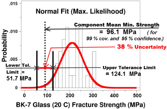
Fit of a normal distribution density function to BK7 glass data.

So, in this paper, we address the size scaling problem by replacing the prediction interval methodology for the test data of specimens with the tolerance interval methodology for predicting the uncertainty of the sample mean for a proportion of the entire set of full-size parts. It is important to note that the current ASTM standard, C 1683-08, “Standard Practice for Size Scaling …” [4], uses physical arguments to scale the 2-parameter Weibull estimates obtained via ASTM C 1239-07 [3] from a component to a larger system. The approach we propose here is to replace the physical arguments with a statistical methodology based on four concepts, namely, the confidence interval, the prediction interval, the tolerance interval, and the coverage. A description of the four concepts with numerical examples and the definitions of the three uncertainty measures, U _n, U _{n
2}, and U _np for the three intervals, is presented in the Appendix.

4. An example to illustrate the methodology for determining the minimum strength of a glass

The above methodology was applied to a borosilicate glass (BK7) whose fracture strength was measured in biaxial flexure (ring-on-ring) [11]. Table 1 shows the data set with a sample size, n, equal to 31. Three functions (normal, two-parameter Weibull, three-parameter Weibull) were used to Kolmorogov-Smirnov (KS) [5] goodness-of-fit criterion was used to determine which of these functions was the best choice for use in the subsequent scaling process. These results are tabulated in Tables 2 and 3. Based on the goodness-of-fit statistic (low values are better) the three-parameter Weibull function is clearly the superior choice.

Table 1
Failure strengths of 31 BK7 glass discs (MPa)

129.83 143.42 149.33 158.79 160.17 165.83 167.69

175.82 175.96 177.89 184.03 184.58 184.65 186.51

190.79 206.16 214.50 228.91 232.57 232.78 233.67

239.67 246.50 247.60 254.98 255.67 255.74 272.90

303.69 312.28 312.90

Table 2

Analysis of glass data using 5 candidate models. These are the best estimates of the strength distribution parameters based upon the available test coupon data

Model	Normal	2-Parameter Weibull	3-Parameter Weibull
Goodness-of-fit statistic	0.151	0.153	0.117 (best)
Location (MPa) parameter	212.4 (mean)	(Non-existent)	121.7 (S _m )
Std. dev.	9.0		12.1
Scale (MPa) parameter	50.0 (s.d.)	232.2 (S ₀)	102.3 (S ₀ )
Std. dev.	6.5	9.5	11.8
Shape parameter		4.64 (m ₂)	1.91 (m ₃ )
Std. dev.		0.65	0.45

Table 3

Prediction of behavior of full-size components at a 95% confidence limit and 99% coverage

	Model
Tolerance limit and confidence	Normal	2-Parameter Weibull	3-Parameter Weibull
Lower tolerance limit (MPa) at 95% confidence	60.0	63.9	118.7
Mean min. strength (MPa)	96.1	86.1	130.9
Uncertainty gap = mean minimum strength − lower tol. limit	36.1	22.2	12.2
Tolerance limit (99% coverage) Uncertainty metric = (uncertainty gap)/(mean min. strength)	0.38 or, 38%	0.26 or, 26%	0.09 or, 9% (lowest)

Further evidence that the 3-parameter Weibull expression is the better fit to the data is demonstrated in Figs 2 and 3. Figure 2 shows the fit for the 2-parameter Weibull. Not only is the predicted minimum component strength quite low (86.1 MPa), but also the uncertainty metric (26%) is very high. On the other hand, for the 3-parameter Weibull fit (Fig. 3), the minimum predicted component strength is higher (130.9 MPa) and the scatter metric is significantly lower (9%).

Fig. 2.

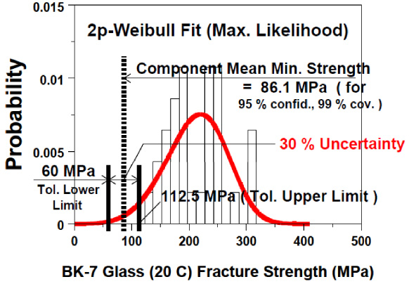
Fit of a 2-parameter Weibull distribution to BK7 glass data.

Fig. 3.

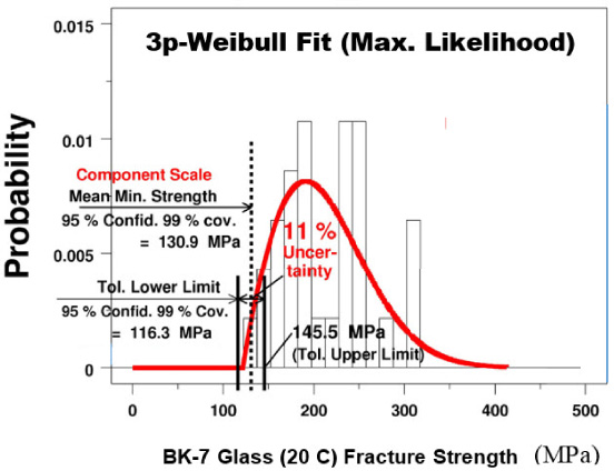
Fit of a 3-parameter Weibull distribution to BK7 glass data.

5. Meaning of the lower tolerance limit in predicting full-size component failure

From Table 3, we can see that, if we choose the best fit function to be the 3-parameter Weibull (3 pW), the lower tolerance limit for the glass based on the testing of the specimens is 118.7 MPa for 99% coverage and a 95% confidence limit. This value was calculated using DATAPLOT. This means that if we consider a large window (or numerous windows) made from this glass, there exists the possibility that 1% of the area of the windows could contain a flaw with a severity that could lead to fracture at this stress. This analysis presumes that all of the windows will be loaded such that the stress over the area of all the windows is uniform, and of the value at which the specimens were loaded. If stresses in parts of an actual window are lower than this, then the prediction given by this calculation is conservative provided no new flaw is introduced.

6. Example of the methodology for other ceramics

The methodology described above was applied to two other ceramics, an aluminum oxide (AD-94, Coors Ceramics) and a sintered silicon nitride (Grade SN W-1000, GTE-Wesgo). Chao and Shetty [6] measured the strengths of each of these materials using three techniques, 3-point flexure, 4-point flexure, and biaxial flexure using a pressurized disc. For brevity we do not list the other three sets of data that included materials tested in both 4-point flexure and biaxial, pressurized discs.¹ Results of our new analysis are summarized in Tables 4, 5, and 6.

Table 4
KS-Max-Likelihood goodness-of-fit statistics for glass, silicon nitride, and alumina

Material Sample size Normal 2-P Weibull 3-P Weibull

BK-7 glass [11] 31 0.151 0.153 0.117 (best)

Silicon nitride 4-pt bend [5] 27 0.115 0.112 0.082 (best)

Silicon nitride pressure disc [5] 32 0.080 (best) 0.110 (Does not exist)

Aluminum oxide [5] 30 0.080 (best) 0.106 (Does not exist)

Material	Sample size	Normal	2-P Weibull	3-P Weibull
BK-7 glass [11]	31	0.151	0.153	0.117 (best)
Silicon nitride 4-pt bend [5]	27	0.115	0.112	0.082 (best)
Silicon nitride pressure disc [5]	32	0.080 (best)	0.110	(Does not exist)
Aluminum oxide [5]	30	0.080 (best)	0.106	(Does not exist)

Table 5

CS-Max-Likelihood goodness-of-fit statistics for glass, silicon nitride, and alumina

Material	Sample size	Normal	2-P Weibull	3-P Weibull
BK-7 glass [11]	31	13.72	13.70	10.61 (best)
Silicon nitride 4-pt bend [5]	27	5.37	7.07	3.69 (best)
Silicon nitride pressure disc [5]	32	4.48 (best)	6.72	5.48
Aluminum oxide [5]	30	0.56 (best)	1.59	0.73

Table 6

Tolerance limit (99% coverage) uncertainty metric (%) for glass, silicon nitride, and alumina

Material	Sample size	Normal	2-P Weibull	3-P Weibull
BK-7 glass [11]	31	38%	26%	9% (lowest)
Silicon nitride 4-pt bend [5]	27	11%	13%	3% (lowest)
Silicon nitride pressure disc [5]	32	8% (lowest)	10%	10%
Aluminum oxide [5]	30	12% (statistically a dead heat)	13% (statistically a dead heat)	11% (statistically a dead heat)

Table 7

Comparison of the “A-basis design allowable stress (MPa)” selected from the 2 pW model (ASTM) approach vs. our approach by making the best choice among 5 models according to a goodness-of-fit or tolerance limit uncertainty metric

	“A-basis” design allowable stress (MPa) for full-size component (95% confidence, 99% coverage)
Data set no., material name, temperature (type of strength test)	2-p Weibull	Our approach (full-size scale, model-selection, goodness-of-fit)	Difference
DS-1. BK-7 glass at 20 C (biaxial test)	60.0	116.3	+94%
DS-2. silicon nitride at 20 C (4-point bend test)	414.2	590.5	+43%
DS-3. silicon nitride at 20 C (biaxial test)	432.1	487.1	+13%
DS-4. aluminum oxide at 20 C (uniaxial test)	239.2	275.7	+15%

7. Significance of the new approach

In this paper and a companion one [9], we propose a new approach of estimating the minimum A-basis-design tensile strength of a full-size component or structure by computing the 95% confidence, 99% coverage, Lower Tolerance Limit (LTL) of a two-metric-validated statistical distribution that “best” represents a given set of fracture strength data obtained from the failure of specimens in a test laboratory. Using four sets of such data from laboratory-scale specimens of three ceramic materials, we illustrate the methodology of our approach by computing the minimum A-basis-design tensile strength of a full-size scale component or structure of those materials and compare our results with the same estimates based on the assumption of a 2-parameter Weibull distribution as shown in Table 7. It is interesting to note that the difference varies widely from a low of 13% to a high of 94%. This result is significant because it suggests that the ASTM approach of assuming a 2-parameter Weibull distribution needs to be modified for an improved design methodology that accounts for the scaling effect in interpreting laboratory-scale data for full-size scale applications.

On the other hand, when we disregard the scaling effect, we find the ASTM approach to be quite comparable to ours, as shown in Table 8, where we use the Lower Prediction Bound (LPB) instead of the Lower Tolerance Limit (LTL) to compute the minimum design tensile strength. In that case, the difference varies from 6% to 12%. However, we believe there is also a significant lesson there, namely, the use of the ASTM approach is equivalent to the assumption that there is no scaling effect – an assumption that is false.

Table 8
Comparison of the minimum strength selected from the 2 pW model (ASTM, laboratory scale) approach vs. our approach by making the best choice among 5 models according to a goodness-of-fit metric for four ceramic materials

Minimum design strength (MPa) (one-sided, 95% confidence, lower limit)

Data set no., material name, temperature (type of strength test) 2-p Weibull approach (ASTM, laboratory-scale) Our approach (laboratory-scale, model-selection, goodness-of-fit) Difference

DS-1. BK-7 glass at 20 C (biaxial test) 96.1 101.8 +6%

DS-2. silicon nitride at 20 C (4-point bend test) 512.6 572.8 +12%

DS-3. silicon nitride at 20 C (biaxial test) 514.4 542.2 +6%

DS-4. aluminum oxide at 20 C (uniaxial test) 301.3 321.6 +7%

	Minimum design strength (MPa) (one-sided, 95% confidence, lower limit)
DS-1. BK-7 glass at 20 C (biaxial test)	96.1	101.8	+6%
DS-2. silicon nitride at 20 C (4-point bend test)	512.6	572.8	+12%
DS-3. silicon nitride at 20 C (biaxial test)	514.4	542.2	+6%
DS-4. aluminum oxide at 20 C (uniaxial test)	301.3	321.6	+7%

8. Discussion on (1) sample size, (2) scaling issue, and (3) relation to stochastic theory of fracture

Issue 1: How many specimens are necessary to assure the statistical accuracy of the proposed methodology?

In mechanical testing for finding the ultimate strength of a structural material, the question on the minimum or optimal number of test specimens needed to obtain credible information about material variability has been of interest for a long time. The statistical methodology proposed in this paper provides us with a quantitative guide to address that question.

As shown in the Appendix, Section A.3., Eq. (11), the tolerance interval is defined as follows: $\begin{eqnarray}m\pm sK_{3},\quad \text{with}∼K_{3}=q({\gamma},n)∼r(n,p),\end{eqnarray}$ where m is the sample mean, s, the sample standard deviation, n, the sample size, 𝛾, the level of confidence, p, the coverage denoting the proportion of the population one is interested in covering, and q and r are two factors depending on 𝛾, n, p as tabulated in the study by Nelson, Coffin and Copeland [15] for two-sided tolerance intervals associated with a normally distributed set of data. For one-sided tolerance intervals that are applicable to reliability studies such as this paper, the factor K can be found tabulated in Natrella’s study [14]. In this paper, we use one-sided tolerance intervals because they are relevant to the estimation of minimal parameters such as the minimum strength of a structural material.

For most applications, we work with a 95% level of confidence and a 99% coverage to estimate the so-called Lower Tolerance Limit (LTL), or the A-basis for design of critical parts in aerospace structures, which is given by the following expression: $\begin{eqnarray}LTL=m-sK_{3}=m(1-K_{3}s/m)=m(1-K_{3}cv),\end{eqnarray}$ where cv is the coefficient of variation defined by s∕m.

In Fig. 4, we show a plot of K ₃ vs n (sample size) for the A-basis design in a black line that levels off at K ₃ approaching the value of 3.0 as n equals 30 or greater. This is a significant observation, because if we wish to end up with an LTL no less than 40% of the sample mean, and the coefficient of variation is no greater than 20%, then a value of 3.0 for K ₃ is acceptable, and a minimum sample size is recommended. However, if we had prior experience with a given material and we knew its cv is much less than 20%, a smaller sample size (<30) may be used without losing the assurance that the statistical methodology is valid.

Fig. 4.

Plot of one-sided tolerance K-factors vs. sample size for 90% and 99% coverages (95% confidence level, normal distribution), after Natrella [14].

Issue 2: What is the cause of the size effect in strength of full-scale engineering structure as the proposed statistical method predicts a tolerance lower limit based solely on data from laboratory-size specimens?

The size effect or the so-called “scaling issue” in mechanical testing of structural materials is addressed in the proposed statistical methodology by introducing the concept of “coverage,” denoted by p, with 0 < p < 1, such that the method is only capable of predicting a minimum design limit for a proportion, p, of the full-scale structure instead of the entire structure. The cause of addressing the size effect is geometric and is not physical in the sense that it does not address the size effect in the material microstructure.

It is, therefore, interesting to observe that our proposed methodology simply uses another geometric assumption to address the size effect when compared with the current method based on ASTM C 1683-08 [4].

Issue 3: What is the correlation between the results obtained by the proposed statistical methodology and those obtained by analyses based on the stochastic theory of fracture [20]?

Using P (t), the probability of crack formation later than time t as a fundamental variable with P (0) = 1, and m (t), the probability per unit time that cracks form at time t as a second variable, the stochastic theory of fracture (see, e.g., [20, p. 22–28]) was able to model both crack initiation and propagation as a rate process with a general predictive framework showing that there was a wide scatter of the ultimate strength data, but there was no minimum as found by Weibull [18]. This means one can choose any form of distribution to represent the ultimate strength dtata and it will not be inconsistent with the stochastic theory of fracture.

In this paper, we developed two statistical metrics to rank the variety of choices of distribution for the ultimate strength data. The two metrics were: a goodness-of-fit criterion and a minimum strength uncertainty criterion. For a numerical implementation of the statistical methodology [9], we limited the number of distributions to five, namely, the Normal, the 2-parameter Weibull, the 3-parameter Weibull, the 2-parameter-Log-Normal, and the 3-parameter Log-Normal. For four brittle materials we reported in this paper with results given in Tables 5 and 6, we found the so-called best choice among all of the first three distributions, namely, the Normal, the 2-parameter Weibull, and the 3-parameter Weibull.

Recognizing that our proposed methodology was developed by using purely mathematical arguments whereas the stochastic theory of fracture [20] was based on physically plausible assumptions, it is interesting to observe that the two approaches yielded results that completely correlate in a qualitative sense.

9. Conclusion

In this paper, we have presented a modern methodology for assessing the fracture probability of ceramic components. The method makes use of the concepts of tolerance limit and coverage to extend the statistical probability of fracture from a laboratory data set to the entire population of full-scale components.

We repeat that a primary assumption in applying this (or any other methodology) to proceed from laboratory strength data to a full-scale component strength distribution is that the flaw distribution in the laboratory set is representative of that in the components. Because of this, it is important that the laboratory data be taken on specimens as similar in geometry to the components as possible in terms of surface preparation, and with the largest convenient stressed area.

This leads to the conclusion that whenever possible biaxial flexural tests, e.g., ring-on-ring, should be chosen over uniaxial flexural tests. If the component is manufactured in the form of a rod or a beam, then other test procedures must be used. Furthermore, our new approach of finding the best-fit distribution for the strength test data based on a least scatter-metric criterion allows us to show that the traditional approach of choosing the 2-parameter Weibull is way too conservative with a side-effect that it would result in an exceedingly low estimate of reliability. Thus, our new methodology will allow the engineer to select the more appropriate degree of mechanical reliability needed to provide safe use of the components.

Footnotes

Acknowledgements

The authors wish to thank N. Alan Heckert and Dr. James J. Filliben of the National Institute of Standards and Technology, Gaithersburg, Maryland, for their technical assistance during this investigation.

Conflict of interest

None to report.

Disclaimer

Certain commercial equipment, instruments, materials, or computer software is identified in this paper in order to specify the experimental or computational procedure adequately. Such identification does not imply recommendation or endorsement by the U.S. National Institute of Standards and Technology, nor is it intended to imply that the materials, equipment, or software identified are necessarily the best available for the purpose.

Confidence interval,prediction interval,tolerance interval and the concept of coverage

Let us begin with a sample data set, $A:\{x_{i}\}$ , i = 1,2, …, n , of n univariate data, where each x _i is real. We also define sample mean, m, and sample standard deviation, s: (4) $\begin{eqnarray}\displaystyle m & = & \displaystyle \left(\sum x_{i}\right)/n,\quad \text{with}∼i=1,2,\ldots ,n.\end{eqnarray}$ (5) $\begin{eqnarray}\displaystyle s & = & \displaystyle \left\{[1/(n-1)]\sum (x_{i}-m)^{2}\right\}^{1/2},\quad \text{with}∼i=1,2,\ldots ,n.\end{eqnarray}$ We are interested in the question: How “good” is the sample mean? To define an uncertainty for the sample mean, U _n, of the set A, we need to introduce a probability distribution, such as the following probability density function of a normal distribution: (6) $\begin{eqnarray}f(x)=\{1/[{\sigma}(2{\pi})^{1/2}]\}\exp [-(x-{\mu})^{2}/(2{\sigma}^{2})],\end{eqnarray}$ where 𝜇 is the population mean, 𝜎, the population standard deviation, and the variable x ranges from minus infinity to plus infinity.

To fix ideas on a fundamental concept of uncertainty, let us select the normal density function, Eq. (6), as the underlying probability distribution. For a normal distribution, it is well-known in the statistics literature (see, e.g., [5,14,15]) that we need to define the following three intervals with the introduction of a numerical quantity, 𝛾, (0 < 𝛾 <1) where 𝛾 is known as the “confidence coefficient” or the “level of confidence”:

1

3-point flexure tests are not recommended for design of components, and so were not analyzed.

References

Aldrich

, R. A. Fisher and the maximum likelihood 1912–1922, Statistical Science 12(3) (1997), 162–176.

Anderson

D.R.

, Model Based Inference in the Life Sciences: A Primer on Evidence, Springer, 2008, pp. 147–154, (Appendix A. Likelihood Theory).

ASTM Designation: C 1239-07, Standard Practice for Reporting Uniaxial Strength Data and Estimating Weibull Distribution Parameters for Advanced Ceramics, Committee C28 on Advanced Ceramics, West Conshohocken, PA 19428-2959, 2008.

ASTM Designation: C 1683-08, Standard Practice for Size Scaling of Tensile Strengths Using Weibull Statistics for Advanced Ceramics, Committee C28 on Advanced Ceramics, West Conshohocken, PA 19428-2959, 2009.

Bury

K.V.

, Statistical Models in Applied Science, Wiley, 1975.

Chao

L.-Y.

and Shetty

D.K.

, Reliability analysis of structural ceramics subjected to biaxial flexure, J. Am. Ceram. Soc. 74(2) (1991), 333–344.

Evans

A.G.

and Wiederhorn

S.M.

, Proof testing of ceramic materials, analytic basis for failure prediction, Int. J. Fract. Mech. 10(3) (1974), 379–392.

Filliben

J.J.

and Heckert

N.A.

, Dataplot: A Statistical Data Analysis Software System, National Institute of Standards and Technology, Gaithersburg, MD, 2002.

Fong

J.T.

Heckert

N.A.

Filliben

J.J.

Marcal

P.V.

and Freiman

S.W.

, Estimation of a minimum allowable structural strength based on uncertainty in material test data, Journal of Research National Institute of Standards and Technology 126 (2021), 126036. doi:10.6028/jres.126.036.

10.

Freiman

S.W.

and Mecholsky Jr

J.J.

, The Fracture of Brittle Materials, 2nd edn, John Wiley and Sons, 2019.

11.

Fuller Jr

E.R.

Freiman

S.W.

Quinn

J.B.

Quinn

G.D.

and Carter

W.C.

, Fracture mechanics approach to the design of glass aircraft windows: A case study, in: Proc. Conf., SPIE – The International Society for Optical Engineering, 26–28 July 1994, San Diego, CA, vol. 2286, 1994, pp. 419–430.

12.

Lau

A.T.C.

, Why 30: A consideration for standard deviation, ASTM Standardization News (2017), 47–48.

13.

Mecholsky Jr

J.J.

Freiman

S.W.

and Rice

R.W.

, Effect of grinding on flaw geometry and fracture of glass, J. Am. Ceram. Soc. 60 (1977), 114–117.

14.

Natrella

M.G.

, in: Experimental Statistics, National Bureau of Standards Handbook, Vol. 91, 1966. (Aug. 1, 1963, reprinted with corrections Oct. 1966) (Superintendent of Documents, U.S. Government Printing Office, Washington, DC 20402), pp. 1-4, 1-15, 2-13, 2-14, and 2-15, Tables A-6 and A-7.

15.

Nelson

P.R.

Coffin

and Copeland

K.A.F.

, Introductory Statistics for Engineering Experimentation, Elsevier, New York, 2003.

16.

Quinn

G.D.

, Fractography of Ceramics and Glasses, NIST Recommended Practice Guide, Special Publication 960-16, 2007.

17.

Quinn

G.D.

and Morrell

, Design data for engineering ceramics: A review of the flexure test, J. Am. Ceram. Soc. 74(9) (1991), 2037–2066.

18.

Weibull

W.A.

, Statistical theory of strength of materials, Ingeniorsvetenskapakad Handl. (151) (1939), 293–297.

19.

Weibull

W.A.

, A statistical distribution function of wide applicability, Journal of Applied Mechanics 18(3) (1951), 293–297.

20.

Yokobori

, The Strength, Fracture and Fatigue of Materials (English edition), P. Noordhoff/Groningen, The Netherlands, 1965.

	Minimum design strength (MPa) (one-sided, 95% confidence, lower limit)
Data set no., material name, temperature (type of strength test)	2-p Weibull approach (ASTM, laboratory-scale)	Our approach (laboratory-scale, model-selection, goodness-of-fit)	Difference
DS-1. BK-7 glass at 20 C (biaxial test)	96.1	101.8	+6%
DS-2. silicon nitride at 20 C (4-point bend test)	512.6	572.8	+12%
DS-3. silicon nitride at 20 C (biaxial test)	514.4	542.2	+6%
DS-4. aluminum oxide at 20 C (uniaxial test)	301.3	321.6	+7%

A new statistical methodology for assessing mechanical survivability of brittle materials

Abstract

Keywords

1. Introduction

3. A 4-step methodology

Table 1 Failure strengths of 31 BK7 glass discs (MPa) 129.83 143.42 149.33 158.79 160.17 165.83 167.69 175.82 175.96 177.89 184.03 184.58 184.65 186.51 190.79 206.16 214.50 228.91 232.57 232.78 233.67 239.67 246.50 247.60 254.98 255.67 255.74 272.90 303.69 312.28 312.90

6. Example of the methodology for other ceramics

Footnotes

Acknowledgements

Conflict of interest

Disclaimer

Confidence interval,prediction interval,tolerance interval and the concept of coverage

1

References

Table 1
Failure strengths of 31 BK7 glass discs (MPa)

129.83 143.42 149.33 158.79 160.17 165.83 167.69

175.82 175.96 177.89 184.03 184.58 184.65 186.51

190.79 206.16 214.50 228.91 232.57 232.78 233.67

239.67 246.50 247.60 254.98 255.67 255.74 272.90

303.69 312.28 312.90