The Aggregate Association Index applied to stratified 2 × 2 tables: Application to the 1893 election data in New Zealand

Abstract

Data aggregation often occurs due to data collection methods or confidentiality laws imposed by government and institutional organisations. This kind of practice is carried out to ensure that an individual’s privacy is protected but it results in selective information being distributed. In this case, the availability of only aggregate data makes it difficult to draw conclusions about the association between categorical variables. This issue lies at the heart of Ecological Inference (EI) and is of growing concern for data analysts, especially for those dealing with the aggregate analysis of a single, or multiple, 2 $\times$ 2 contingency tables. Currently, there are a number of EI approaches that are available and provide the analyst with tools to analyse aggregated data but their success has been mixed due to the variety of assumptions that are made about the individual level data, or the models that are developed to analyse them.

As an alternative to ecological inference, one may consider the Aggregate Association Index (AAI). This index gives the analyst an indication of the likely association structure between two categorical variables of a single 2 $\times$ 2 contingency table when the individual level, or joint frequency/proportion, data is unknown. To date, the AAI has been developed for the analysis of a single 2 $\times$ 2 table. Hence, the purpose of this paper is to extend the application of the AAI to the case where aggregated data from multiple 2 $\times$ 2 tables (i.e. stratified 2 $\times$ 2 tables) require analysis. To illustrate this new extension of the AAI, New Zealand voting data in 1893 is studied with the focus on gender. This data comprises of fifty-five electorates where the data available consists of the marginal information of a 2 $\times$ 2 table. The importance of this New Zealand voting data is that it was in this 1893 election where gender equality in voting at a national level was recognised for the first time in the world.

Keywords

2 × 2 tables aggregate data marginal information ecological inference Aggregate Association Index

1. Introduction

The 2 $\times$ 2 contingency table is the most fundamental data structure used when cross-classifying dichotomous variables. It is therefore not surprising that the analysis of this particular data structure has received a considerable amount of attention in the statistical and allied literature; see, for example, [1, 2]. Most of the attention to date has focused on the case when cell values are known. However, due to the imposition of confidentiality restrictions imposed on the individual-level data by government and organisational institutions, or because of problems with the availability of individual-level data during the data collection process, the aggregate data (i.e. marginal totals) of a single 2 $\times$ 2 contingency table, or multiple 2 $\times$ 2 contingency tables, are increasingly available.

When dealing with the analysis of aggregated categorical data, the utilisation of such data can be traced back to Fisher’s comments in 1935, see [3, page 48], where he stated:

“Let us blot out the contents of the table, leaving only the marginal frequencies. If it be admitted that these marginal frequencies by themselves supply no information on the point at issue, namely, as to the proportionality of the frequencies in the body of the table we may recognize that we are concerned only with the relative probabilities of occurrence of the different ways in which the table can be filled in, subject to these marginal frequencies.”

These comments suggest that the marginal frequencies are not important for inferring the unknown cell values of a 2 $\times$ 2 contingency table. They have also generated much discussion on the analysis of aggregate data. For example, Yates [4] agreed with Fisher’s comments but stipulated that they are true “except in extreme cases and in repeated sampling”. Furthermore, Yates’ inference [4] about the association between two dichotomous variables at the individual-level given only the availability of aggregate data (for multiple 2 $\times$ 2 tables) has been well discussed by Chambers and Steel [5]. Plackett [6], Aitkin and Hinde [7] and Barnard [8] also agreed with Fisher’s comments. Goodman [9, 10] overcame the limitation of marginal frequencies in Fisher’s comments by introducing an “ecological regression” technique for multiple 2 $\times$ 2 tables. The aim of his approach is to estimate the cell proportions of a set of 2 $\times$ 2 tables given only the marginal frequencies. However, there are two critical disadvantages when using Goodman’s ecological regression method: (1) the assumption of no aggregation bias and (2) it can yield impossible estimates (e.g. negative values) of the cell frequencies [11]. In 1991, Freedman et al. [12] presented their “neighbourhood model” which overcomes the disadvantages of Goodman’s approach. Although it too suffers from problems concerning the assumptions imposed upon the unknown cell frequencies. The discussions raised by Yates, Goodman and Freedman et al. can be seen as three early attempts at performing ecological inference (EI) which aims to estimate individual-level behaviour given only the availability of aggregate data when analysing multiple 2 $\times$ 2 tables. For more details on the ecological inference, one can refer to, for example, Hudson et al. [11].

The popularity and dissemination of many methods and computational platforms for the analysis of aggregated categorical data increased significantly after King [13] introduced his suite of EI techniques in 1997. King et al. [14] introduced new EI methodologies including the use of Markov Chain Monte Carlo methods to extend King’s 1997 ecological inference approaches. Steel et al. [15] introduced the homogeneous model designed to overcome many of the assumptions underlying the previous EI techniques developed.

More recently, Greiner and Quinn [16] proposed a method to analyse the association between the variables of a general R $\times$ C tables given only the marginal information. Hudson et al. [11] compared several popular EI techniques including those of Goodman [9, 10], Freedman et al. [12], King’s parametric and non-parametric ecological inference [13], Chambers and Steel [5], and the homogeneous models of Steel et al. [15]. Comparisons were made in terms of the goodness-of-fit between the estimated values and the known true values of the cell frequencies. From their study, Hudson et al. [11] stated that “all EI methods make assumptions about the data to compensate for the loss of information due to aggregation”. For more details, one can also refer to Salway and Wakefield [17] for a common EI framework, Imai et al. [18] for a Bayesian and likelihood approach to the analysis of multiple 2 $\times$ 2 ecological tables, Glynn and Wakefield [19] for ecological inference in social sciences and Xu et al. [20] for methodological challenges in climate change epidemiology.

In terms of software, EI and EzI were developed by King [21, 22] to perform a range of EI techniques described in his 1997 book and include diagnostics and graphical outputs. In the R programming language, one can also refer to the package eco by Imai et al. [23] for the EI of multiple 2 $\times$ 2 tables or eiPack by Lau et al. [24] for R $\times$ C tables.

Despite the growing number of solutions to, and discussions of issues concerned with, EI the proposed techniques require imposing untestable assumptions on the unknown individual-level data. To overcome this problem Beh [25] proposed an alternative strategy by developing the Aggregate Association Index (AAI). The AAI in an index that is bounded by $[0,\,100]$ and assesses whether an association is statistically significant (or not) between two dichotomous variables given only the availability of the marginal, or aggregate, data of a 2 $\times$ 2 table. At a given level of significance, $\alpha$ , an AAI that is close to zero indicates that there is virtually no information in the marginal totals to suggest that an association exists between the two variables. In contrast, an AAI value close to 100 suggests that such an association is likely to exist. However, Beh’s [25, 26] development of the AAI is largely confined to the analysis of a single 2 $\times$ 2 table. The analysis of stratified 2 $\times$ 2 tables using the AAI has been performed in the past [27]; however, there has been no attempt yet to unite the features of the AAI for multiple, or stratified, 2 $\times$ 2 contingency tables.

Therefore, this paper will provide an extension of the AAI for the analysis of multiple, or stratified, 2 $\times$ 2 tables. We shall describe the extension by first describing the 1893 New Zealand voting data and the notation that will be adopted (Section 2). The 1893 New Zealand data is studied because it plays a significant role in the history of gendered voting research and provides a relevant data structure for the analysis of stratified 2 $\times$ 2 tables. Section 3 describes the homogeneity testing of New Zealand women’s preference for voting when the cell frequencies of all electorates in 1893 are known while Section 4 provides an brief overview of EI and the AAI. Sections 5 and 6 will provide new insight into the AAI by describing how the index, and its key graphical features, can be extended for studying stratified 2 $\times$ 2 tables. Some final comments on these new developments and future work will be discussed in Section 7.

2. 1893 New Zealand voting data

2.1 The data

Prior to 1893, women were not granted the right to cast a formal vote at national elections or referendum anywhere around the world. As a result, “suffragettes” were organised to fight for equal voting rights. The word “suffragette” was first used in a British newspaper article in 1906 to describe women seeking the right to vote through organised protest (http://www.tchevalier.com/fallingangels/bckgrnd/suffrage). On September 19, 1893, the Govenor General of New Zealand, Lord Glasgow, signed a new Electoral Act into law. This Act marked a milestone in New Zealand legislation since it meant that New Zealand became the first self-governing country in the world where all women had the right to vote in parliamentary elections. Even though women in New Zealand were not eligible to stand as candidates until 1919, the trend was quickly spread across the globe. From an Australian perspective, the state of South Australia enfranchised women’s voting right in 1894, Western Australia in 1899, while the Australian federal and the New South Wales governments enacted equal gender voting rights in 1902. After 1902, other Australian states joined the movement, including Tasmania in 1903, Queensland in 1905 and Victoria in 1908 (AUSFOLIO Volume 2, Number 1 SOCOM Educational Resources 1993).

In February 1918, the British government introduced an Act giving women their right to vote if their age was at least 30 years and either possessed property or rented for at least $\pounds$ 5/year; or were the wife of someone who did. Ten years later, in 1928, the British government gave all women over the age 21 the right to vote for the first time in its history. Prior to 1920, suffrage was not popular in the United States except for in various states and localities, the US did not provide equal gender voting at the national level until 1920. Following the British, many European countries, including Denmark, Iceland, the USSR, the Netherlands, Austria, Poland, Sweden, Germany and Luxembourg, also granted the right to women by 1920. Other European countries did not grant women the right to vote until much later; namely, Spain in 1931, France in 1944, Belgium, Italy and Romania in 1947. Countries in Asia were also involved with the change. For example, Japan and Vietnam allowed women to vote in 1946, Singapore in 1947, China in 1949, and Malaysia in 1957. For a comprehensive list of women’s suffrage on an international stage, refer to http://womenshistory.about.com/od/suffrage/a/intl_timeline.htm. Historical documents about New Zealand suffrage can also be found at http://www.nzhistory.net.nz/politics/womens-suffrage and a detailed description of suffrage and the fight for equal voting rights between the genders can be found in Moore [28].

The data used in this paper is reproduced from https://atojs.natlib.govt.nz/cgi-bin/atojs by permission of the National Library of New Zealand. It summaries the results of the New Zealand general election held on November 28, 1893 and the Maori election of December 20, 1893. This document can be viewed online at https://atojs.natlib.govt.nz/cgi-bin/atojs?a=d&d=AJHR1894-I.2.3.2.21. The New Zealand voting scene in 1893 can be encapsulated as follows: the country’s population at that time was approximately 626,359 people. Sixty-six electorates were formed in the 1893 election consisting of 62 general electoral districts and 4 Maori electoral districts. There were 302,997 registered electors in the 1893 election with the official turnout rate of 75.3% (http://www.elections.org.nz/events/past-events/general-elections-1853-2014-dates-and-turnouthttp://www.elections.org. nz/events/past-events/general-elections-1853-2014-dates-and-turnout).

In the 1893 election, the first national election where men and women were given equal rights to vote, 90,290 women visited polling booths across New Zealand to exercise their right. This figure represents 82.5% of the number of women who registered to vote at the election; a significant turnout at the start of women suffrage movement. A closer examination of the 1893 New Zealand data reveals that there were four metropolitan electorates (the cities of Auckland, Wellington, Christchurch and Dunedin) where the number of votes recorded was more than the number of names listed on the role of registered voters. There were three electorates (Westland, Bruce and Awarua) where only one candidate stood for election and so there was no contest and the four Mauri electorates did not record the number of voters. Therefore, of the original 66 electorates throughout New Zealand, data were only available from 55 electorates, which will be the focus of our discussion and analysis. The voter turnout of the male and female voters in the 55 electorates of the 1893 election are summarised in the 2 $\times$ 2 table of Table 1.

Table 1
1893 New Zealand voter turnout summary by gender

Gender/Turnout	Voted	Didn’t Vote	Total
Female	66,743	10,992	77,665
Male	103,448	46,512	175,915
Total	170,191	57,434	227,625

Fortunately for analysts studying aggregate data, the number of men and women who did, and did not, turnout to vote was recorded for each electorate. Therefore, Table 1 can be modified to yield 55 stratified 2 $\times$ 2 tables where, for each electorate, the Gender (Female and Male) and Turnout (Voted and Didn’t Vote) are cross-classified to form an electorate-level 2 $\times$ 2 table. With the advantage of having a complete data set, it is possible to compare the results from two different perspectives: (1) when the joint cell frequencies of each table are known, and (2) when these cell values are unknown and only the aggregate, or marginal, information for each electorate is available.

Table 2

Notation for the cell, and marginal, frequencies, of the $g$ ’th 2 $\times$ 2 table

Gender/Turnout	Voted	Didn’t vote	Total
Female	$n_{11g}$	$n_{12g}$	$n_{1\bullet g}$
Male	$n_{21g}$	$n_{22g}$	$n_{2\bullet g}$
Total	$n_{\bullet 1g}$	$n_{\bullet 2g}$	$n_{g}$

2.2 Notation

For each of the 55 New Zealand electorates that we are studying, a 2 $\times$ 2 contingency table can be formed. Table 2 shows the notation used to describe the joint, and marginal, cell frequencies of the 2 $\times$ 2 table for the $g$ ’th electorate, for $g=$ 1, 2, $\ldots$ , 55. Denote the total number of registered individuals in the $g$ ’th electorate by $n_{g}$ and the total number of registered individuals in New Zealand by $N=\sum_{g=1}^{G}n_{g}$ where $G=$ 55 is the total number of electorates under examination in the 1893 New Zealand election. Let the joint frequency of individuals classified into the $i$ ’th row and $j$ ’th column (for $i=$ 1, 2 and $j=$ 1, 2) of the $g$ ’th 2 $\times$ 2 table be $n_{ijg}$ with an electorate proportion of $p_{ijg}=n_{ijg}/n_{g}$ . Define the $i$ ’th row marginal proportion and the $j$ ’th column marginal proportion be denoted by $p_{i\bullet g}=p_{i1g}+p_{i2g}$ and $p_{\bullet jg}=p_{1jg}+p_{2jg}$ , respectively.

For the New Zealand voting data, the row variable consists of the gender categories Female ( $i=$ 1) and Male ( $i=$ 2). The column variable reflects whether a registered individual “Voted” ( $j=$ 1) or “Didn’t Vote” ( $j=$ 2).

For the $g$ ’th electorate, denote $P_{1g}=n_{11g}/n_{1\bullet g}$ to be the conditional probability of an individual being classified into Column 1 (Vote) given that they are classified as Female in Row 1. The proportion of women in all of the 55 New Zealand electorates who turned out to vote, $P_{1}$ , can be easily calculated based on the electorate level data such that

$\displaystyle P_{1}=\frac{\sum\limits_{g=1}^{G}n_{11g}}{\sum\limits_{g=1}^{G}n% _{1\bullet g}}.$ (1)

3. Homogeneity testing of the conditional proportions

P_{1g}

when cell values are known

When the cell frequencies of each of the 2 $\times$ 2 tables are known, a test of homogeneity can be performed on the conditional proportions $P_{1g}$ to assess whether the turnout of the women voters in the 1893 New Zealand election are consistent from one electorate to another. Klein and Linton [29] discussed several procedures for performing such tests. These include Pearson’s test [30], the likelihood ratio test [31], exact conditional (ExactC) and unconditional tests described by Agresti [32, 33, 34], a test based on moment matching chi-squared approximations [35, 36] and a normal approximation for sparse data [37].

From their review, Klein and Linton [29] showed that the ExactC test, Nass test (Nass [35]) and Xu test (Xu [37]) exhibited equally reliable performance in the simulation study undertaken. Furthermore, Klein and Linton [29] found that the ExactC test and Nass test perform equally well. However, the ExactC implies complexity when stratum sample size and the number of strata are large. For simplicity, the ExactC test shall not be considered further in this study due to the large sample size and large number of the electorates in 1893. Therefore, we consider here the Nass and Xu tests of homogeneity of the $P_{1g}$ for the 1893 voting data. Table 3 shows that both of these tests recommend rejecting the null hypotheses of equal conditional proportions $(P_{1g})$ for all electorates. Hence, there is sufficient statistical evidence to suggest that the New Zealand women’s preference for voting differs significantly from one electorate to another electorate in the 1893 election.

4. The analysis of stratified 2 $\times$ 2 tables when cell values are unknown

4.1 Ecological Inference (EI)

While Section 3 considered the case where the cell frequencies at the electorate level are known, consider now the case where this information is assumed unknown. In general, ecological inference allows for the analyst to draw individual-level (at the joint cell frequency/proportion level) conclusions given only the aggregate, or marginal, information [13, 14, 38, 39, 11]. Obviously, a wide range of different numbers could be substituted for the cell values without contradicting its row and column marginals. This logic is referred to in the literature as the method of bounds – see [40] for more details. Furthermore, there are potentials of drawing incorrect conclusions (i.e. paradoxes) at an individual level when using only the aggregate-level data. These paradoxes are well-known to data analysts when working with unknown-cell-value contingency tables and can be summarised as ecological fallacy, Yule-Simpson’s paradox and aggregation bias.

The first issue when drawing individual-level conclusions given only the aggregate-level data is “ecological fallacy”[41, 38]. This states that the result of a particular study at an aggregate level (e.g. election year) does not necessarily imply the same result at an individual level (e.g. voters from different electorates – Table 2). Individual-level information is often lost in the process of aggregation, and thus, all EI methods make assumptions about the data to compensate for the loss of information [11].

The second issue is “Yule-Simpson’s paradox” [42, 43]. This is a situation in which individual-level conclusions derived from different groups may be reversed when the groups are combined. For the 1893 NZ election, it means that the association between the variables at the electorates may be opposite to that at the year level. The Yule-Simpson’s paradox can be minimised when causal relations are brought into consideration [44]. For a more comprehensive history and understanding of the Yule-Simpson’s paradox, one can refer to [45, 46].

Figure 1.

Graphical illustration of the AAI concept for the 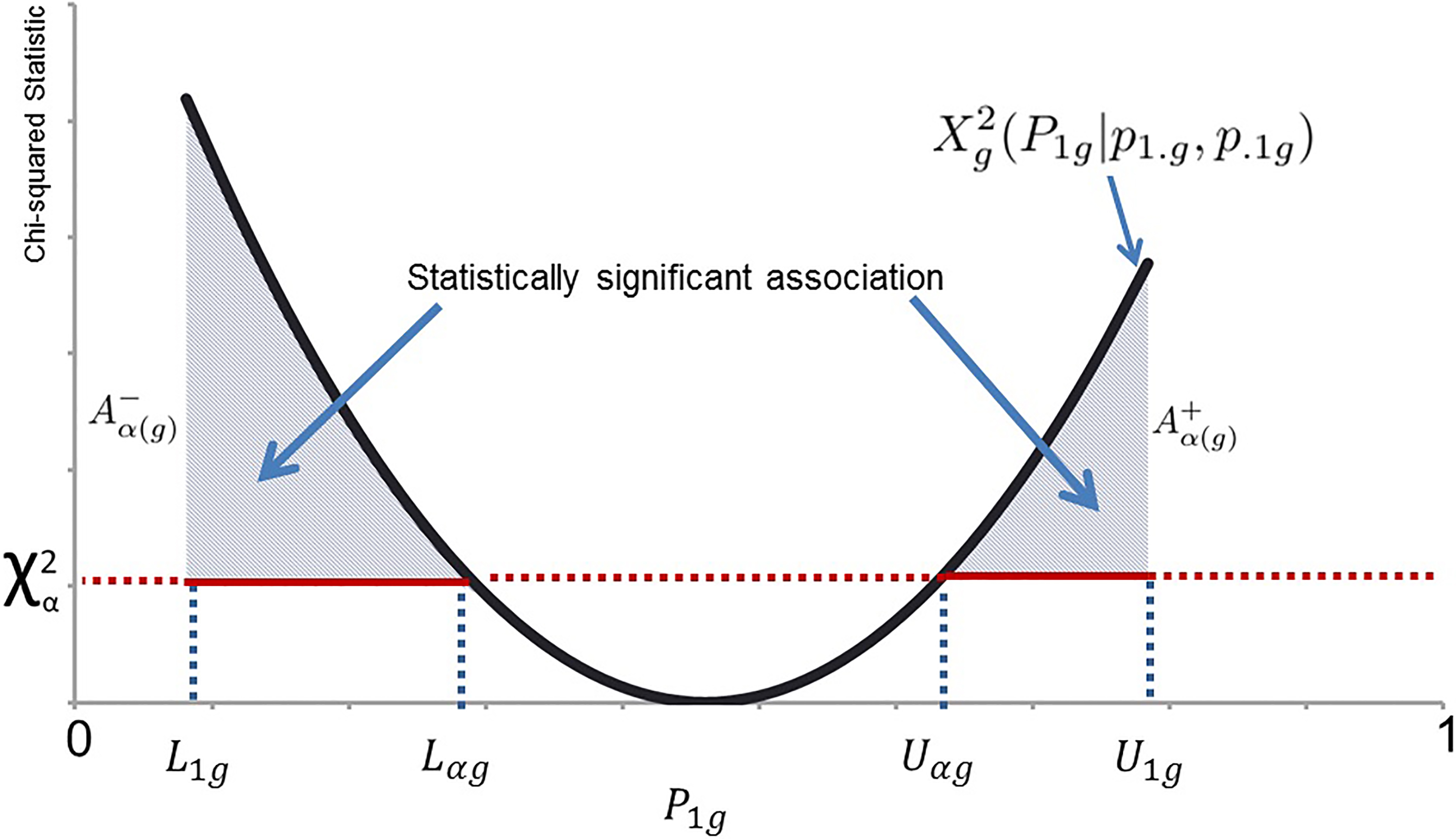$g^{th}$ electorate.

The third issue is the “aggregation bias”. Specifically, aggregation bias refers to the discrepancies between the expected values of estimators using the aggregate-level data and estimators using the indivi-dual-level data [11]. For multiple contingency tables, this occurs when the conclusions at the aggregate level does not accurately reflect the underlying association between the variables at the individual level. In King’s book [13, Chapter 9.2], he stated that this paradox is one of many main difficulties in providing accurate results in ecological inference and proposed several approaches to detect, assess and avoid aggregation bias.

To date, the ecological inference problem is still among the more widely encountered statistical problems in social sciences and other sectors such as epidemiology, geography, sociology, economics, and history research [39, 14]. To overcome the difficulty in ensuring the integrity of the untestable assumptions in EI, and the paradoxes given only marginal information, Beh [25, 26] proposed an alternative approach named as Aggregate Association Index (AAI). The AAI and its extension are the main focus of this study and shall be discussed further in Sections 4.2, 5 and 6.

4.2 Aggregate Association Index (AAI)

Analysing the association between two or more categorical variables typically requires answering at least one of the following three questions:

Is there sufficient evidence in the sample to infer that a statistically significant association exists between the categorical variables?

What is the best measure to quantify the direction of the association between the variables?

What appropriate techniques can be used to visualise the association between the variables?

For the 1893 New Zealand election data, the first question can be answered by performing a Pearson chi-squared test of independence between Gender and Turnout. For the $g$ ’th electorate, the Pearson chi-squared statistic is:

$\displaystyle X_{g}^{2}=n_{g}\frac{({n_{11g}n_{22g}-n_{12g}n_{21g}})^{2}}{n_{1% \bullet g}n_{2\bullet g}n_{\bullet 1g}n_{\bullet 2g}}.$ (2)

and the statistical significance of the statistics can be assessed by comparing $X_{g}^{2}$ against the $1-\alpha$ percentile of the chi-squared distribution with 1 degree of freedom.

A simple, yet popular, means of answering the second question is to assess the direction and magnitude of the association between the variables using Pearson’s product moment correlation. This correlation, defined for the $g$ ’th electorate as

$\displaystyle r_{g}=\frac{n_{11g}n_{22g}-n_{12g}n_{21g}}{\sqrt{n_{1\bullet g}n% _{2\bullet g}n_{\bullet 1g}n_{\bullet 2g}}}$ (3)

takes on a value ranging from $-$ 1 to 1 where $r_{g}=$ $\pm$ 1 implies a perfect (linear) association exists between the variables, while $r_{g}=$ 0 implies no association between Gender and Turnout at the $g$ ’th electorate.

To answer the third question, correspondence analysis (CA) can be performed to provide a visual depiction of the association between the two or more categorical variables. Very little attention has been paid to the case of performing a correspondence analysis on a 2 $\times$ 2 table, although Beh [25] studied the properties for the analysis for aggregate data. For a comprehensive discussion on correspondence analysis, the reader is directed to, for example, Greenacre [47] and Beh and Lombardo [48].

While these strategies are commonly used to study the association between categorical variables when the cell frequencies of Table 2 are known, they are not appropriate for the analysis of aggregate data. Although, when only the marginal information of a single 2 $\times$ 2 table are available, Beh [25, 26] proposed the Aggregate Association Index (AAI) to overcome the difficulty of assessing the association between two dichotomous variables. Here, we expand upon Beh’s [25, 26] index by studying its features for the simultaneous analysis of stratified 2 $\times$ 2 tables.

Consider the definition of $P_{1g}=n_{11g}/n_{1\bullet g}$ described in Section 2.2. Beh [25, 26] showed that, for the $g$ ’th electorate, Pearson’s chi-squared statistic can be expressed as a function of $P_{1g}$ and the marginal information such that

$\displaystyle X_{g}^{2}(P_{1g}|p_{1\bullet g},p_{\bullet 1g})=$ (4) $\displaystyle\ \ \ \ \ n_{g}\left(\frac{P_{1g}-p_{\bullet 1g}}{p_{2\bullet g}}% \right)^{2}\Bigg{(}\frac{p_{1\bullet g}p_{2\bullet g}}{p_{\bullet 1g}p_{% \bullet 2g}}\Bigg{)}\,.$

The quadratic function of Fig. 1 is a graphical depiction of Eq. (4.2) with respect to $P_{1g}$ – this curve shall be referred to as the AAI curve of the 2 $\times$ 2 table.

When only marginal information is known, the value of $P_{1g}$ is well understood to lie within the bounds (Duncan and Davis [40])

$\displaystyle L_{1g}=\max\Bigg{(}0,\frac{p_{\bullet 1g}-p_{2\bullet g}}{p_{1% \bullet g}}\Bigg{)}\leqslant P_{1g}\leqslant\min\Bigg{(}\frac{p_{\bullet 1g}}{% p_{1\bullet g}},1\Bigg{)}=U_{1g}.$ (5)

Table 3

Homogeneity test results – Nass test and Xu tests

Year	Nass Test	Nass P-value	Xu Test	Xu P-value
1893	1,518.90	$<$ 0.000001	139.57	$<$ 0.000001

Since $L_{1g}$ and $U_{1g}$ only depend on the aggregate data, the features of the chi-squared statistic $X_{g}^{2}(P_{1g}|p_{1.g},p_{.1g}$ ) defined by Eq. (4.2) can be studied given only this aggregate data. Beh [25, 26] showed that when only the aggregate data of a 2 $\times$ 2 table is available, and a test of the statistical significance of the association is made at the $\alpha$ level of significance, the bounds of $P_{1g}$ are

$\displaystyle L_{\alpha g}=\max\Bigg{(}0,p_{\bullet 1g}-p_{2\bullet g}\sqrt{% \frac{\chi_{\alpha}^{2}p_{\bullet 1g}p_{\bullet 2g}}{n_{g}p_{1\bullet g}p_{2% \bullet}}}\Bigg{)}\leqslant P_{1g}\leqslant\min\!\!\Bigg{(}p_{\bullet 1g}+p_{2% \bullet g}\sqrt{\frac{\chi_{\alpha}^{2}p_{\bullet 1g}p_{\bullet 2g}}{n_{g}p_{1% \bullet g}p_{2\bullet g}}},1\!\!\Bigg{)}=U_{\alpha g}.$ (6)

Given the aggregate data, one may therefore conclude that there exists a statistically significant association between Gender and Turnout at the $g$ ’th electorate, and at the $\alpha$ level of significance, if $L_{1g}\leqslant P_{1g}\leqslant L_{\alpha g}$ or $U_{\alpha g}\leqslant P_{1g}\leqslant U_{1g}$ . Conversely, there is no evidence of a statistically significant association between the two dichotomous variables if $L_{\alpha g}\leqslant P_{1g}\leqslant U_{\alpha g}$ .

By taking into account the above properties of $P_{1g}$ , Beh [25, 26] proposed the Aggregate Association Index (AAI). For the $g^{th}$ electorate, the AAI is defined as

$\displaystyle A_{\alpha g}=100(1-[(L_{\alpha g}-L_{1g})+(U_{1g}-U_{\alpha g})]% \chi_{\alpha}^{2}+\text{Int}(L_{\alpha g},U_{\alpha g})/\text{Int}(L_{1g},U_{1% g}))$ (7)

where $\mathrm{Int}(a,b)=\int\limits_{a}^{b}X_{g}^{2}(P_{1g}|p_{1\bullet g},p_{% \bullet 1g})\,\mathrm{d}P_{1g}$ .

For a given level of significance, $\alpha$ , the AAI is the ratio of the total region that lies under the quadratic curve defined by Eq. (4.2) but which is above the critical value of $\chi_{\alpha}^{2}$ with 1 degree of freedom. Given only the marginal information, this index therefore quantifies how likely a statistically significant association exists between the two dichotomous variables at the $\alpha$ level of significance. Figure 1 provides a graphical representation of the AAI.

The index $A_{\alpha g}$ in Eq. (7) is bounded by [0, 100] where a value of zero indicates that, at the $\alpha$ level of significance, there is no evidence of a statistically significant association between the variables. On the other hand, a value close to 100 indicates that, at the $\alpha$ level of significance, there is sufficient evidence to suggest that such an association exists. Beh [26] showed that the AAI index can also be partitioned such that $A_{\alpha g}=A_{\alpha g}^{+}+A_{\alpha g}^{-}$ . Here

$\displaystyle A_{\alpha g}^{+}\!=\!100\!\left(\!\!\frac{\int\limits_{U_{\alpha g% }}^{U_{1g}}\Big{[}X_{g}^{2}(P_{1g}|p_{1\bullet g},p_{\bullet 1g})\!-\!\chi_{% \alpha}^{2}\Big{]}\text{d}P_{1g}}{\int\limits_{L_{1g}}^{U_{1g}}X_{g}^{2}(P_{1g% }|p_{1\bullet g},p_{\bullet 1g})\text{d}P_{1g}}\!\!\right)$ (8)

is referred to as the aggregate positive association index (AAI $+$ ), which measures the extent to which the marginal information reflects a positive association. The magnitude of this index is reflected by the area under the AAI curve (and above the critical value) that is to the right of its vertex. In contrast,

$\displaystyle A_{\alpha g}^{-}\!=\!100\!\left(\!\!\frac{\int\limits_{L_{1g}}^{% L_{\alpha g}}\Big{[}X_{g}^{2}(P_{1g}|p_{1\bullet g},p_{\bullet 1g})\!-\!\chi_{% \alpha}^{2}\Big{]}\text{d}P_{1g}}{\int\limits_{L_{1g}}^{U_{1g}}X_{g}^{2}(P_{1g% }|p_{1\bullet g},p_{\bullet 1g})\text{d}P_{1g}}\!\!\right)$ (9)

is referred to as the aggregate negative association index (AAI $-$ ), which quantifies the extent to which the marginal information reflects a negative association. The magnitude of this index is reflected by the area under the AAI curve (and above the critical value) that is to the left of its vertex.

The discussions of the AAI made by Beh [25, 26] were confined to the analysis of aggregate data for a single 2 $\times$ 2 table although, as we show in the remainder of this paper, its application can be extended to the case where multiple 2 $\times$ 2 tables are simultaneously analysed. In doing so, Section 5 shall discuss a procedure for determining an overall AAI curve derived from multiple AAI curves. We shall also discuss how one may cluster AAI curves to identify electorates with homogeneous voter turnout between the two genders, given only the availability of the aggregate data at each electorate (Section 6). Therefore, the following sections describe an approach that allows for the simultaneous analysis of stratified aggregate data using the AAI curves of all of the electorates to provide a single overall AAI curve for the 1893 New Zealand election data. Figure 2 provides a graphical depiction of the AAI curves for all 55 New Zealand electorates in the 1893 election. When testing the association between Gender and Turnout, at the electorate level, for $\alpha=0.05$ , the AAI at each electorate is above 99.0. This suggests that, for all electorates, it is very likely that a statistically significant association exists between the two dichotomous variables. Furthermore, since the AAI curves are more dominant on the left side of the vertex than on the right side, Fig. 2 shows that the association between Gender and Turnout for most of the electorates is negative. This implies that, registered voters who were male, were more likely to turnout and vote than female registered voters.

Figure 2.

AAI curves from the 55 electorates in the 1893 New Zealand election.

While not the focus of this paper, the large AAI may be a result of either the large sample size or the configuration of the marginal information (or a combination of both). For more information on this issue, the interested reader is directed to Beh et al. [49] who introduced two strategies that help assess and minimise the impact of an increasing sample size of a 2 $\times$ 2 contingency table on the AAI. Another related issue is the assessment of the real magnitude of the AAI for a given sample size; see Cheema et al. [50]. We shall not discuss this issue here.

5. Overall AAI curve for stratified 2

\times

2 tables

5.1 The overall AAI curve

While Fig. 2 shows that, for each electorate of the 1893 New Zealand election, we can gain an understanding of voting behaviour between the genders from only the aggregate data, it is also of interest to determine the characteristics of the AAI and AAI curve for that year. By doing so provides some insight into variations from one election period to another based on limited information through the aggregate data. Such further insights will be left for further discussion, but a preliminary study of this issue has been undertaken by Beh et al. [27]. For example, since the AAI of each electorate in the 1893 New Zealand data is at least 99.0 this suggests that the (overall) AAI for year 1893 will exceed 99.0. To examine how an overall AAI may be determined for the 55 electorates, consider Pearson’s chi-squared defined for the $g$ ’th electorate by Eq. (4.2). It may be alternatively, but equivalently, expressed as a quadratic function in terms of $P_{1g}$ such that

$\displaystyle X_{g}^{2}(P_{1g}|p_{1\bullet g},p_{\bullet 1g})=\left(\frac{n_{g% }p_{1\bullet g}}{p_{\bullet 1g}p_{\bullet 2g}p_{2\bullet g}}\right)\left(P_{1g% }-p_{\bullet 1g}\right)^{2}.$ (10)

Before we derive an expression for the overall AAI for the 1893 election, consider first that the equation of a general functional form of a parabola at a point $(x,y)$ is

$\displaystyle y=a\left(x-h\right)^{2}+k,$ (11)

where $a$ is the leading coefficient, $\left(h,\,k\right)$ are the coordinates of the vertex and $\left(h,\,k+1/(4a)\right)$ is the focus of the parabola; see, for example, Anton [51] for more details.

By comparing Eq. (10) with Eq. (11), the leading coefficient of the AAI curve for the $g$ ’th electorate is $(n_{g}p_{1\bullet g})/(p_{\bullet 1g}p_{\bullet 2g}p_{2\bullet g})$ . The vertex’s coordinates of Eq. (10) can be found as

$\displaystyle\left(p_{\bullet 1g},0\right)$ (12)

and the focus’s coordinates are

$\displaystyle\left(p_{\bullet 1g},\frac{p_{\bullet 1g}p_{\bullet 2g}p_{2% \bullet g}}{4n_{g}p_{1\bullet g}}\right).$ (13)

The curvature coefficient of the AAI curve at the vertex point can also be defined as

$\displaystyle\gamma_{g}=\frac{2np_{1\bullet g}}{p_{2\bullet g}p_{\bullet 1g}p_% {\bullet 2g}}.$ (14)

The key features of the AAI’s quadratic function, just like all quadratic functions, are the bounds of $P_{1g}$ defined by Eq. (5), the vertex defined by Eq. (12), the focus defined by Eq. (13) and the curvature at the vertex point defined by Eq. (14).

In terms of the simultaneous depiction of the AAI curves given in Fig. 2, we shall now turn our attention to finding the “best” overall AAI curve for the 1893 election. Section 5.2 describes how this overall AAI curve can be found.

5.2 Finding an overall curve

Since there are 55 electorates in the 1893 New Zealand election, there are also 55 vertex points and 55 focus points. Therefore, the mean vertex point is

$\displaystyle\Bigg{(}\frac{1}{G}\sum_{g=1}^{G}p_{\bullet 1g},0\Bigg{)},$ (15)

where $G$ ( $=$ 55) is the number of electorates. Similarly, the mean focus point is

$\displaystyle\Bigg{(}\frac{1}{G}\sum_{g=1}^{G}p_{\bullet 1g},\frac{1}{G}\sum_{% g=1}^{G}\frac{p_{\bullet 1g}p_{\bullet 2g}p_{2\bullet g}}{4n_{g}p_{1\bullet g}% }\Bigg{)}.$ (16)

Note that, when calculating these mean quantities, we give equal weight to each of the $G=$ 55 electorates. Weighting each electorate equivalently is consistent with how stratified data is analysed in EI. For example, calculating the overall $P_{1}$ using Eq. (1) treats each electorate the same. There may be situations where some electorates may be weighted more heavily than others, but we shall leave this issue for further consideration. The leading coefficient, $a$ , of the fitted overall AAI curve can be defined as:

$\displaystyle a=\frac{1}{4d},$ (17)

where $d$ is the distance between the mean vertex point and the mean focus point:

$\displaystyle d=\frac{1}{4G}\sum_{g=1}^{G}\frac{p_{\bullet 1g}p_{\bullet 2g}p_% {2\bullet g}}{n_{g}p_{1\bullet g}}.$ (18)

Therefore, when only the aggregate data is available at the electorate level, the overall AAI curve for the 1893 New Zealand election can be defined by the chi-squared statistic

$\displaystyle X^{2}(P_{1})=\left(\frac{G}{\sum\limits_{g=1}^{G}\frac{p_{% \bullet 1g}p_{\bullet 2g}p_{2\bullet g}}{n_{g}p_{1\bullet g}}}\right)\Bigg{(}P% _{1}-\frac{1}{G}\sum_{g=1}^{G}p_{\bullet 1g}\Bigg{)}^{2},$ (19)

where $P_{1}$ is given by Eq. (1).

Since an AAI curve, depicted by Eq. (4.2), is bounded by Eq. (5), the overall AAI curve defined by Eq. (19) also requires restriction on its bounds. The overall bounds can be defined in terms of the marginal information by

$\displaystyle L_{1}=\max\left(0,\frac{\sum\limits_{g=1}^{G}p_{\bullet 1g}-\sum% \limits_{g=1}^{G}p_{2\bullet g}}{\sum\limits_{g=1}^{G}p_{1\bullet g}}\right)% \leqslant P_{1}\leqslant\min\left(\frac{\sum\limits_{g=1}^{G}p_{\bullet 1g}}{% \sum\limits_{g=1}^{G}p_{1\bullet g}},1\right)=U_{1}\,.$ (20)

Figure 3.

Overall AAI curve (dashed line) for the 1893 New Zealand election.

See, for example, Hudson, Moore et al. [11].

When testing the association between the dichotomous variables at the $\alpha$ level of significance, the bounds of $P_{1}$ are

$\displaystyle L_{\alpha}=\max$ $\displaystyle\ \ \ \ \left(0,\frac{1}{G}\sum\limits_{g=1}^{G}p_{\bullet 1g}-% \sqrt{\frac{\chi_{\alpha}^{2}}{G}\sum\limits_{g=1}^{G}\frac{p_{\bullet 1g}p_{% \bullet 2g}p_{2\bullet g}}{n_{g}p_{1\bullet g}}}\right)$ $\displaystyle\ \ \ \ \leqslant P_{1}\leqslant\min$ (21) $\displaystyle\ \ \ \left(\frac{1}{G}\sum\limits_{g=1}^{G}p_{\bullet 1g}+\sqrt{% \frac{\chi_{\alpha}^{2}}{G}\sum\limits_{g=1}^{G}\frac{p_{\bullet 1g}p_{\bullet 2% g}p_{2\bullet g}}{n_{g}p_{1\bullet g}}},1\right)$ $\displaystyle\ \ \ =U_{\alpha}.$

Therefore, by utilising Eq. (19), we can also determine the AAI for the 1893 election, across all electorates, at the level of significance $\alpha$ . The overall AAI for the 1893 election is

$\displaystyle A_{\alpha}=100\left(1-\frac{\left[(L_{\alpha}-L_{1})+(U_{1}-U_{% \alpha})\right]\chi_{\alpha}^{2}}{\mathrm{Int}(L_{1},U_{1})}\right.\left.-% \frac{\mathrm{Int}(L_{\alpha},U_{\alpha})}{\mathrm{Int}(L_{1},U_{1})}\right),$ (22)

where $\mathrm{Int}(a,b)=\int\limits_{a}^{b}X^{2}(P_{1})\,\mathrm{d}P_{1}$ . This AAI can be partitioned into its AAI $+$ and AAI $-$ terms to assess the likely direction of the association between Gender and Turnout for the 1893 election. The general terms for quantifying AAI $+$ and AAI $-$ are

$\displaystyle A_{\alpha}^{+}=100\left(\frac{\int\limits_{U_{\alpha}}^{U_{1}}% \Big{[}X^{2}(P_{1})-\chi_{\alpha}^{2}\Big{]}\,\mathrm{d}P_{1}}{\int\limits_{L_% {1}}^{U_{1}}X^{2}(P_{1})\,\mathrm{d}P_{1}}\right),$ (23)

and

$\displaystyle A_{\alpha}^{-}=\left(\frac{\int\limits_{L_{1}}^{L_{\alpha}}\Big{% [}X^{2}(P_{1})-\chi_{\alpha}^{2}\Big{]}\,\mathrm{d}P_{1}}{\int\limits_{L_{1}}^% {U_{1}}X^{2}(P_{1})\,\mathrm{d}P_{1}}\right),$ (24)

respectively.

Therefore, given only the marginal information that is available in the stratified data of the 1893 New Zealand election, the overall AAI curve for the 1893 election can be determined from Eq. (19) and is

$\displaystyle X^{2}(P_{1})=10,830.80(P_{1}-0.750)^{2},$ (25)

where 0.260 $\leqslant P_{1}\leqslant 1$ .

Figure 4.

Four clusters of the AAI curves in the 1893 New Zealand election by mclust [1–4: cluster number].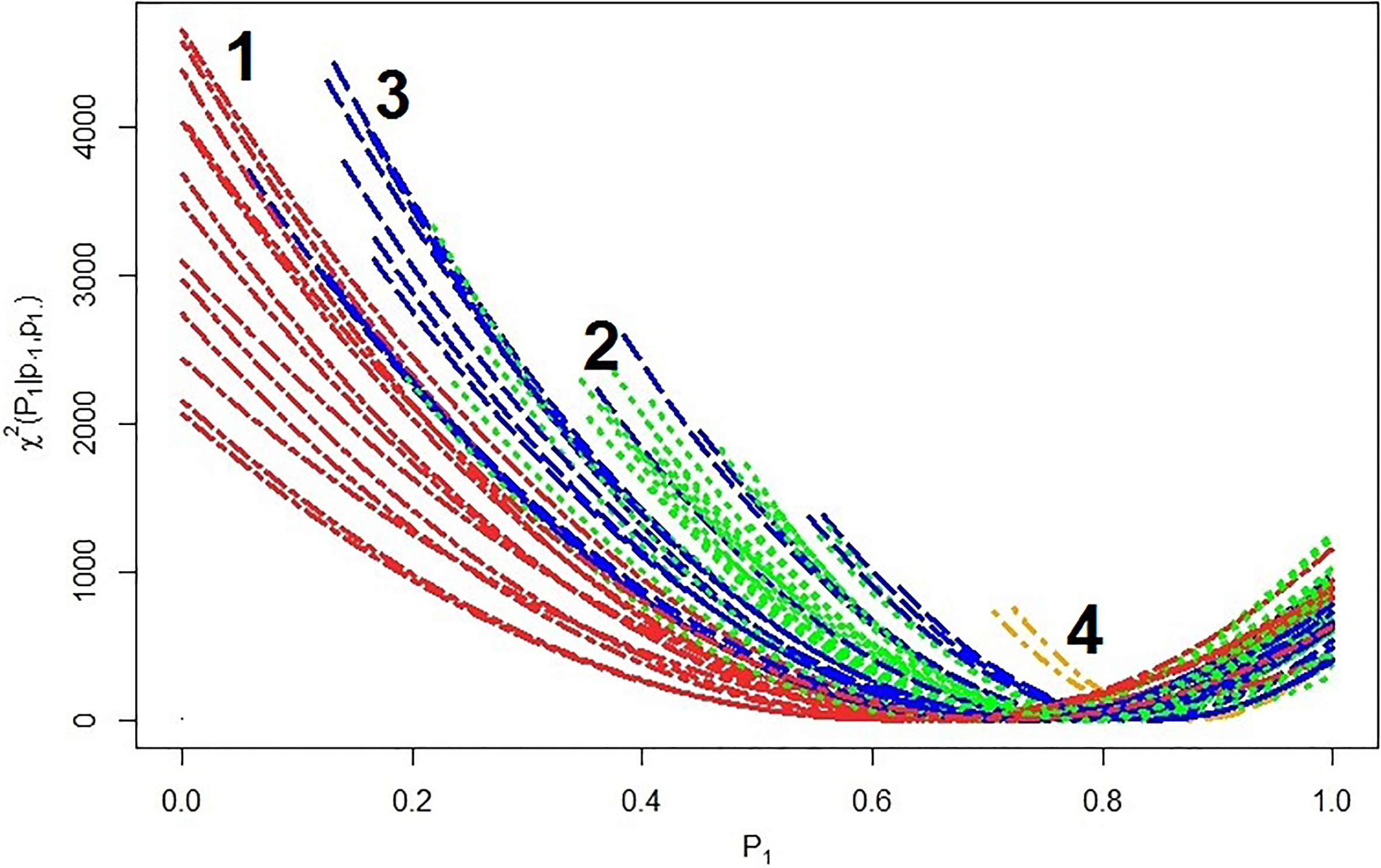

The AAI curve of Eq. (25) is given by the quadratic relationship between the chi-squared statistic and $P_{1}$ defined by Eq. (1). This AAI curve appears as the dashed line in Fig. 3. At the 5% level of significance, the overall AAI for the 1893 election is 99.40 and clearly shows that there is a high possibility of a statistically significant association between Gender and Turnover across all of the 55 electorates. Partitioning the AAI produces $A_{\alpha}^{+}=$ 12.32 and $A_{\alpha}^{-}=$ 87.08. These terms suggest that the overall association between the two variables, Gender and Turnout is seven times more likely to to be negative than positive. Therefore, using only the aggregate data of the 1893 New Zealand election, a registered male voter was more likely to turnout and vote than a registered female voter.

6. Clustering electorate level AAI curves

6.1 Bounds, vertex, and curvature

When only the aggregate data is available for analysis, the analyst may not just be interested in determining the AAI for specific electorates. Instead, there may also be interest in determining clusters of electorates that exhibit homogeneous, or heterogeneous, voting behaviors. There are a number of methodologies that may be considered for clustering electorates. These include, but are not limited to, hierarchical clustering [52, 53], centroid-based clustering [53, 54] and model-based clustering [53]. However, despite the popularity of many of these techniques, Fraley and Raftery [55] have pointed out some fundamental issues that are not dealt with using traditional cluster analysis procedures. These issues include, but are not restricted to, objectively identifying how many clusters should be considered, which of the variety of clustering approaches should be used and when, and how outliers are to be dealt with. To remedy these, and other interrelated issues, Fraley and Raftery [55] have proposed a clustering technique based on selecting the best Bayesian model using the Bayesian information criteria (BIC) [56]. The framework of their approach lies with the Gaussian mixture model and the wide selection of models that stem from the eigen-decomposition of the covariance matrix, $\Sigma$ . In R, this technique can be applied using the R package mclust [57]. To identify clusters of homogeneous voting behaviour amongst our 55 New Zealand electorates using this method, three characteristics of an AAI curve shall be considered:

The bounds of an AAI curve for the $g$ ’th electorate, $\left(L_{1g},\,U_{1g}\right)$ ,

The vertex of the quadratic function that defines an AAI curve Eq. (12), and

The curvature coefficient of an AAI curve Eq. (14).

For the 1893 election, the values of $U_{1g}$ are identical for all of the electorates and so we shall consider only $L_{1g}$ as the information contained in the bounds. However, depending on the data being studied, the upper bound for the $g$ ’th electorate/strata may need to be considered for the determination of the clusters. Note also that, for the vertex of the AAI curve $\left(p_{\bullet 1g},\,0\right)$ , the ordinate of zero is identical for each electorate and so, for clustering purposes, the x-coordinate of the vertex ( $p_{\bullet 1g}$ ) shall be considered.

6.2 Model-based Clustering using mclust

In order to study the features of the electorate-specific AAI curves, we shall be using the software package mclust[57] in R to study the curves bounds, vertex and curvature. This package performs model-based clustering, classification, and density estimation based on finite normal mixture modelling. The package considers the overall population as a mixture of groups or clusters and each component of this mixture is modeled through its conditional probability distribution. It implements a number of different data models and applies maximum likelihood estimation and Bayesian criteria to identify the most likely model and number of clusters. Since complex models can often explain the data better than a simple model, this makes choosing the most suitable model inherently challenging. mclust uses Bayesian Information Criterion (BIC) [56] to select the optimal mixture model. In particular, the larger the value of the BIC, the stronger is the evidence for the model and number of clusters. As a result, clusters are defined as groups of objects based on how likely the objects belong to the same distribution.

Figure 5.

Fitted cluster-specific AAI curves (solid lines) and fitted election-specific AAI curve (dashed line) for the 1893 New Zealand election [1–4: cluster number].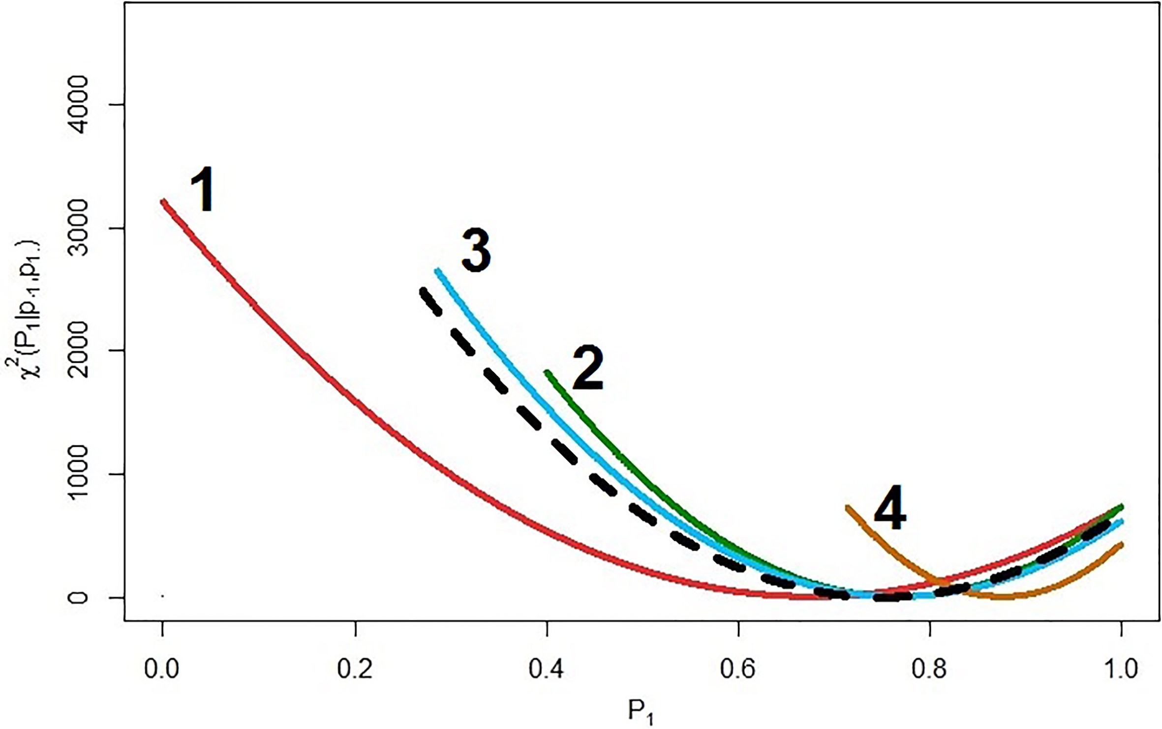

Table 4

AAI, AAI+ and AAI- for the fitted electorate-specific curves and election-specific curve in the 1893 New Zealand election

Cluster	n	AAI	AAI+	AAI-
1	13	99.5373	9.7403	89.7970
2	24	99.2128	20.055	79.1578
3	16	99.4411	9.9828	89.4583
4	2	99.1899	30.648	67.5420
All Electorates	55	99.4027	12.3157	87.0870

When clustering the characteristics of the AAI curve outlined in Section 6.1 for the electorates of the 1893 New Zealand election, mclust identifies four distinct clusters under the VEV model (Ellipsoidal Distribution with Equal Shape), with a Bayesian Information Criterion (BIC) of $-$ 843.0357. The number of electorates per cluster can be referred to in Table 4 while Fig. 4 shows how the clusters of the electorates (obtained from using mclust) can be used to identify homogeneous voting behaviour given only the aggregate data. In particular, this figure shows there are four clusters of the AAI curves. Cluster 1 consists of the AAI curves for 13 electorates that are deemed to have homogeneous association between Gender and Turnout. Figure 4 also visually reflects the 24 electorates (Cluster 2) that are identified using mclust to have a homogeneous voting behavior. Similar comments can also be made regarding the analysis of aggregate data from the remaining electorates that are classified either into Cluster 3 (consisting of 16 electorates) or Cluster 4 (consisting of 2 electorates). Table S1 of the supplementary material for this paper lists the cluster in which each of the New Zealand electorates has been classified.

Since mclust has identified four distinct clusters of voting behaviour, we can apply the procedure outlined in Section 5.2 to derive the overall AAI curve for each of the four clusters and for all electorates. Figure 5 shows the overall AAI curve for each of the electorates where their curve is given as a solid coloured line. The overall AAI curve for the 55 electorates shown in Fig. 3 is superimposed on Fig. 5.

Now that the overall AAI curves for each of the four clusters has been determined and graphically depicted in Fig. 5, we can now find the AAI of each cluster as well as their AAI+ and AAI- quantities. Table 4 provides a summary of these values for the four cluster-specific AAI curves and one election-specific AAI curve. It is immediately clear from this table that, given only the marginal information, there is evidence of a strong association between the voters’ gender and whether they turned out to vote in the 1893 New Zealand election. In fact, this association is far more likely to be negative than positive suggesting that registered male voters were more likely to turnout and vote than female registered voters.

The strength of the positive and negative association is not the same for each of the identified clusters. For example, Clusters 1 and 3 are far more likely to exihibit a negative association structure between the two variables than Clusters 2 and 4. While Clusters 1 and 3 are nearly 10 times more likely to have a negative association than a positive association, Cluster 2 is only 4 times more likely to have such an association structure while a negative association in Cluster 4 is only about 3 times more likely than a positive one.

To provide a better understanding of the electorates’ voting behaviour in terms of geographical distribution when only analysing the aggregate data, the electoral district boundaries were approximated by using the region information in https://en.wikipedia.org/wiki/New_Zealand_general_election,_1893#Electorate_results and the mclust classification result was projected onto the New Zealand map as shown in Fig. 6. This figure suggests that the spatial variation of the electorates can be studied to determine any possible homogeneity, or heterogeneity, of voting behaviour in the 1893 election.

Figure 6.

New Zealand map with 1893-election electorates clustered by mclust [1–4: cluster number].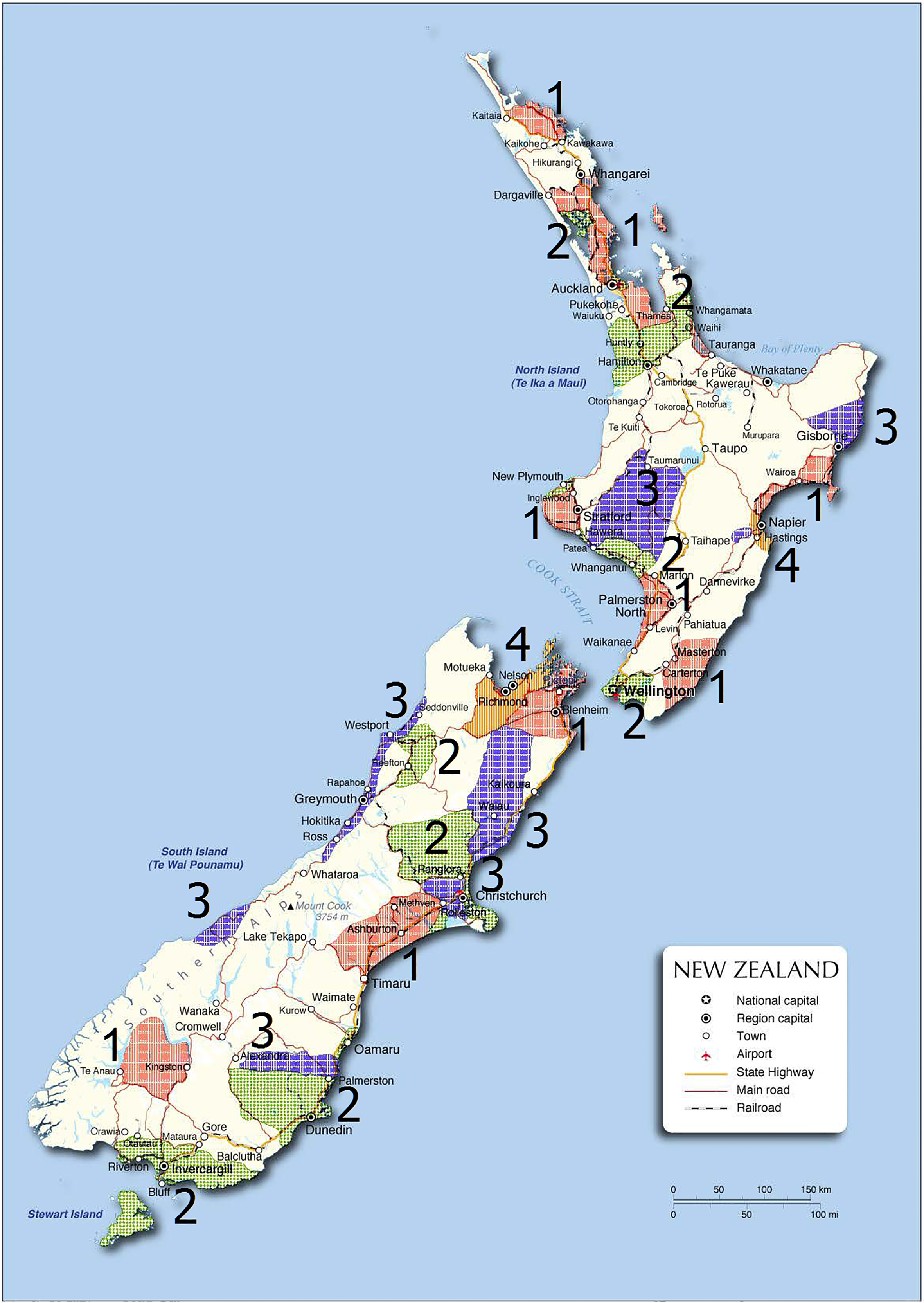

As seen from Fig. 6, the red region (cluster 1), the green region (cluster 2) and the blue region (cluster 3) are geographically close to each other, especially the green and blue region (reflected by the clustering result in Fig. 4) while the two outliers are near Richmond and Napier (cluster 4).

To help understand the source of variation of the electorates among the four clusters, we have undertaken further preliminary studies of the aggregate data. These studies suggest that the population size did not provide any source of homogeneity, or heterogeneity, of the electorates in terms of association. Nor is it apparent that geographical characteristics (e.g. North Island vs South Island, or Rural vs Urban) defined the variation in the voting behaviour between the electorates. However, we have identified that potential sources of clustering may indeed be related to the given aggregate data. The supplementary material provided indicates that the number of voter turnout divided by the number of those that did not turn out $\left(n_{\bullet 1g}/n_{\bullet 2g}\right)$ helps identify the four clusters of electorates. It is clear from the side-by-side boxplot of Fig. S1 that, generally, electorates classified into clusters 2 and 3 have similar voted/did not vote ratio’s but have higher ratios than those electorates in cluster 1 and much lower ratio’s than the two electorates in cluster 4. Thus one potential source of association may be that there is a higher propensity for voter turnout as we move from electorates that appear in cluster 1 to those electorates that appear in cluster 4. A second, and more simple, source that helps to pin-point potential factors that classify voting behaviour between the genders of the electorates into the clusters identified is the proportion of registered individuals that turned out to vote. The side-by-side boxplot of Fig. S2 in the supplementary material suggests that Clusters 1 through to 4 consist of electorates with an increasing proportion of registered individuals who turned out to vote. While these sources provide an initial understanding of how the differences in the clusters can be interpreted, further research into this issue will need to be undertaken. Of course, without further information on the nature of the voting behaviour, whether it be through partial information of the cell frequencies, or through other extraneous factors, identifying such sources of variation between the clusters remains a challenge.

One may also be interested in understanding what effect the two “outlying” electorates that make up cluster 4 – in the Richmond and Napier regions – have on the membership of clusters 1 to 3. If these electorates are removed from the study, mclust identifies clusters 1 to 3 to be identical to their original formation with one exception – electorate Tuapeka (in the Otago region of the South Island) moved between two clusters.

7. Discussion

By focusing on the analysis of the aggregate data for a single 2 $\times$ 2 contingency table proposed by Beh [26] (see also Section 4.2 for an overview), this paper has extended this earlier work by showing that the Aggregate Association Index (AAI) can be extended in two ways for the analysis of stratified 2 $\times$ 2 tables. Firstly, it can be used as a foundation to determine the overall AAI curve for stratified data (see Section 5) and, secondly, Beh’s [26] approach can be amended to cluster multiple AAI curves (see Section 6).

This paper has shown that, given only the aggregate data of the 1893 New Zealand voting behavior data at the electorate level, there is a statistically significant association between the gender of a registered voter and whether they turned out to vote. Homogeneous voting behaviours amongst the electorates can be identified and visually depicted by clustering via the mclust package in R (Figs 4 and 5) and mapping (Fig. 6). Since the cell values are available at the electorate level in this study, testing for homogeneity of the conditional proportion at the $g$ ’th electorate, $P_{1g}$ , confirms that there does indeed exist differences in voting behaviour across the 55 electorates (see Section 3). When studying only the aggregate data, this finding is reflected by the difference among the AAI curve for each of the electorates as shown in Figs 4 and 6 respectively. As a result, this study has provided a foundation to further investigate what may contribute to the classification of the electorates by considering additional demographic information (e.g. population, age, ethnicity, knowledge of languages, disabilities, home ownership and employment status). One can refer to Hudson et al. [58, 11] and Moore [28] to further study the New Zealand voting data from 1893 and beyond.

Alternative applications of the AAI can be made in a variety of research areas. The extension studied in this paper can be carried out in areas of study including, but not limited to, marketing research, social and medical sciences; these disciplines have commonly used a variety of ecological inference techniques to study their data. Further methodological advances to the AAI and the clustering issues outlined in this paper will also prove beneficial for the practical analysis of aggregated data. For example, the connection between the AAI with other well-known association indices - such as the odds ratio, independence ratio, Pearson’s ratio, the standardised and adjusted residuals (see, for example, [34, 48]) show that the AAI is flexible for a variety of commonly used measures of association the analyst wishes to use; see, also, Beh, Tran and Hudson [59] and Lombardo and Beh [60] for discussions related to such developments. Adapting this work for stratified data will enhance the utility of the AAI in this case.

Further advances to the AAI can be made by generalising Beh’s index [26], his related work, and this paper’s outcomes to the analysis of a single, and stratified $R\times C$ tables, where $R\geqslant 2$ and $C\geqslant 2$ . One important aspect of such expansion may include investigating how to summarise the association test results from multiple $R\times C$ tables to capture the overall association between the categorical variables. This will be left for future work.

Footnotes

Supplementary data

The supplementary files are available to download from https://dx-doi-org.web.bisu.edu.cn/10.3233/SJI-170387.

References

Pearson

. On the theory of contingency and its relation to association and normal correlation. Drapers’ Company Research Memoirs. 1904; 1: 1-36.

Ferguson

. Statistical analysis in psychology and education. New York: McGrawHill, 1966.

Fisher

. The Logic Of Inductive Inference. Journal of the Royal Statistical Society. 1935; 98: 39-82.

Yates

. Test of significance for 2 × 2 contingency tables. Journal of Royal Statistical Society, Series A. 1984; 147: 426-463.

Chambers

Steel

. Simple methods for ecological inference in 2 × 2 tables. Journal of the Royal Statistical Society: Series A. 2001; 163(1): 175-192.

Plackett

. The Marginal Totals of a 2 × 2 Table. Biometrika. 1977; 64(1): 37-42.

Aitkin

Hinde

. Comments to “Tests of significance for 2 × 2 Contingency Tables”. Journal of Royal Statistical Society, Series A. 1984; 47: 453-454.

Barnard

. Comments to “Tests of Significance for 2 × 2 Contingency Tables”. Journal of Royal Statistical Society, Series A. 1984; 47: 449-450.

Goodman

. Ecological regressions and behavior of individuals. American Sociological. 1953; 18(6): 663-664.

10.

Goodman

. Some Alternatives to Ecological Correlation. The American Journal of Sociology. 1959; 64(6): 610-625.

11.

Hudson

Moore

Beh

Steel

. Ecological Inference Techniques: An Empirical Evaluation Using Data Describing Gender and Voter Turnout at New Zealand Elections, 1893–1919. Journal of Royal Statistical Society, Series A. 2010; 173(1): 185-213.

12.

Freedman

Klein

Sacks

Smyth

Everett

. Ecological regression and voting rights. Evaluation Review. 1991; 15(6): 673-711.

13.

King

. A Solution to the Ecological Inference Problem: Reconstructing Individual Behavior from Aggregate Data. Princeton, USA: Princeton University Press, 1997.

14.

King

Rosen

Tanner

. Ecological Inference – New Methodological Strategies. New York: Cambridge University Press, 2004.

15.

Steel

Beh

Chambers

. The information in aggregate data. Ecological Inference: New Methodological Strategies (eds King, G, Rosen, O, Tanner M A). 2004; p. 51-68.

16.

Greiner

Quinn

. R × C ecological inference: bounds, correlations, flexibility and transparency of assumptions. Journal of the Royal Statistical Society: Series A. 2009; 172(1): 67-81.

17.

Salway

Wakefield

. A common framework for ecological inference in epidemiology, political science and sociology. Ecological Inference: New Methodological Strategies (eds King, G, Rosen, O, Tanner M A). 2004; p. 303-332.

18.

Imai

Strauss

. Bayesian and likelihood inference for 2 × 2 ecological tables: an incomplete-data approach. Political Analysis. 2008; 16: 41-69.

19.

Glynn

Wakefield

. Ecological inference in the social sciences. Statistical Methodology. 2010; 7(3): 307-332.

20.

Xun

Khan

Michael

Vineis

. Climate change epidemiology: methodological challenges. International Journal of Public Health. 2010; 55(2): 85-96.

21.

King

. EI: A Program for Ecological Inference. 2003; Available from: http//gking.harvard.edu/ei.

22.

Benoit

King

. EzI: A(n Easy) Program for Ecological Inference. 2003 Available; from: http//gking.harvard.edu/EzI.

23.

Imai

Strauss

. eco: R package for Ecological Inference in 2 × 2 tables. Journal of Statistical Software. 2011; 42(5): 1-23.

24.

Lau

Moore

Kellermann

. eiPack: R × C Ecological Inference and Higher-Dimension Data Management. New Functions for Multivariate Analysis. 2006; 18(1): 43.

25.

Beh

. Correspondence Analysis of Aggregate Data: The 2 × 2 Table. Journal of Statistical Planing and Inference. 2008; 138: 2941-2952.

26.

Beh

. The Aggregate Association Index. Computational Statistics and Data Analysis. 2010; 54: 1570-1580.

27.

Beh

Tran

Hudson

Moore

. Clustering of stratified aggregated data using the aggregate assocation index: Analysis of New Zealand voter turnout (1893–1919). Analysis and Modeling of Complex Data in Behavioral and Social Sciences, 2014.

28.

Moore

. Was gender a factor in voter participation at New Zealand elections? In: M F, E O, editors. Class, Gender and the Vote: Historical Perspectives for New Zealand. Dunedin: University of Otago Press; 2005; p. 129-142.

29.

Klein

Linton

. On a comparison of tests of homogeneity of Binomial proportions. Research report Series – Statistics US Census Bureau. 2013; p. 417-451.

30.

Pearson

. Experimental discussion of the (χ2, P) test of goodness of fit. Biometrika. 1932; 24: 351-381.

31.

Wilks

. The likelihood test of independence in contingency tables. Biometrika. 1928; 20A: 263-294.

32.

Agresti

. A Survey of Exact Inference for Contingency Tables. Statistical Science. 1992; 7: 131-153.

33.

Agresti

. Exact inference for categorical data: Recent advances and continuing controversies. Statistics in Medicine. 2001; 20: 2709-2722.

34.

Agresti

. Categorical Data Analysis. 2nd; ed. John Wiley and Sons; 2002.

35.

Nass

CAG

. The χ2 test for small expectations in contingency tables, with special reference to accidents and absenteeism. Biometrika. 1959; 46: 365-385.

36.

Potthoff

Whittinghill

. Testing for homogeneity: I. The binomial and multinomial distributions. Biometrika. 1966; 53: 167-182.

37.

. Statistical issues in meta-analysis [PhD. diss.]. Department of Mathematics and Statistics. Baltimore County; 2011; Available from: http//search.proquest.com/docview/876965319?accountid=10499.

38.

Freedman

. Ecological Inference and the Ecological Fallacy. International Encyclopedia of the Social and Behavioral Sciences. 1999; 549. Available from: wwwstat.berkeley.edu/∼census/549.pdf.

39.

Schuessler

. Ecological inference. Proceedings of the National Academy of Sciences of the United States of America. 1999; 96(19): 10578-10581. Available from: http//www.

40.

Duncan

Davis

. An Alternative to Ecological Correlation. American Sociological Review. 1953; 18(6): 665-666.

41.

Kramer

. The Ecological Fallacy Revisited: Aggregate-versus Individual-level Findings on Economics and Elections, and Sociotropic Voting. The American Political Science Review. 1983; 1: 92-111.

42.

Simpson

. The interpretation of interaction in contingency tables. Journal of the Royal Statistical Society, Series B; 13(2).

43.

Yule

. Notes on the theory of association of attributes in statistics. Biometrika. 1903; 2(2): 121-134.

44.

Arah

. The role of causal reasoning in understanding Simpsonâ€™s paradox, Lordâ€™s paradox, and the suppression effect: Covariate selection in the analysis of observational studies. Emerging Themes in Epidemiology. 2008; 5(1): 1-5. Available from: http//www.ete-online.com/content/5/1/5.

45.

Hernan

Clayton

Keiding

. The Simpson’s paradox unraveled. International Journal of Epidemiology. 2011; 40: 780-785.

46.

Pearl

. Understanding Simpson’s Paradox. The American Statistician. 2014; 88: 8-13.

47.

Greenacre

. The Theory and Application of Correspondence Analysis. London: Academic Press; 1984.

48.

Beh

Lombardo

. Correspondence Analysis: Theory, Practice and New Strategies. Wiley; 2014.

49.

Beh

Cheema

Tran

Hudson

. In: Carpita M, Brentari E, Qannari EM, editors. Adjustment to the aggregate association index to minimise the impact of large samples. Springer; 2014; p. 241-251.

50.

Cheema

Beh

Hudson

. On the quantification of statistical significance of the extent of association projected on the margins of 2 × 2 tables, when only the aggregate data is available: A pseudo p-value approach – applied to leukaemia relapse data. In: Weber T, McPhee MJ, Anderssen RS, editors. MODSIM2015, 21th International congress on Modelling and Simulation; 1997. p. 1682-1688.

51.

Anton

. Calculus. 3rd ed. John Wiley and Sons; 1988.

52.

Ward

. Hierarchical Grouping to Optimize an Objective Function. Journal of the American Statistical Association. 1963; 58: 236-244.

53.

Hastie

Tibshirani

Friedman

. The Elements of Statistical Learning. 2nd ed. Springer Series in Statistics; 2009.

54.

Niraj

Lade

Malviya

. Clustering of Datasets by using Centroid Based Method. International Journal of Emerging Technology and Advanced Engineering. 2013; 3(5): 614-620.

55.

Fraley

Raftery

. Model-based Clustering, Discriminant Analysis and Density Estimation. Journal of the American Statistical Association. 2002; 97(458): 611-631.

56.

Schwarz

. Estimating the dimension of a model. The Annals of Statistics. 1978; p. 461-464.

57.

Fraley

Raftery

Murphy

Scrucc

. Mclust version 4 for R: Normal mixture modeling for Model-based clustering, classification, and density estimation. Technical Report. 2012; 597. Available from: https//www.stat.washington.edu/research/reports/2012/tr597.pdf.

58.

Hudson

Moore

Beh

Steel

. Gendered counts of historical voting in NZ 1893–1919: A rigorous statistical ecological inference approach. 55

{}^{\rm th}

session of the International Statistical Institute (ISI) (Invited Special Session). 2005; p. 1-4.

59.

Beh

Tran

Hudson

. A reformulation of the Aggregate Association Index using the Odds Ratio. Computational Statistics and Data Analysis. 2013; 68: 52-65.

60.

Lombardo

Beh

. The prediction index for aggregate data. Journal of Applied Statistics. 2016; 43(11): 1998-2018.

The Aggregate Association Index applied to stratified 2 × 2 tables: Application to the 1893 election data in New Zealand

Abstract

Keywords

1. Introduction

2. 1893 New Zealand voting data

2.1 The data

Table 1 1893 New Zealand voter turnout summary by gender

4. The analysis of stratified 2 × 2 tables when cell values are unknown

4.1 Ecological Inference (EI)

5.1 The overall AAI curve

6.1 Bounds, vertex, and curvature

6.2 Model-based Clustering using mclust

Footnotes

Supplementary data

References

Table 1
1893 New Zealand voter turnout summary by gender

4. The analysis of stratified 2 $\times$ 2 tables when cell values are unknown