Reconciliation of inconsistent data sources using hidden Markov models

Abstract

This paper discusses how National Statistical Institutes (NSI’s) can use hidden Markov models (HMMs) to produce consistent official statistics for categorical, longitudinal variables using inconsistent sources. Two main challenges are addressed: first, the reconciliation of inconsistent sources with multi-indicator HMMs requires linking the sources on the micro level. Such linkage might lead to bias due to linkage error. Second, applying and estimating HMMs regularly is a complicated and expensive procedure. Therefore, it is preferable to use the error parameter estimates as a correction factor for a number of years. However, this might lead to biased structural estimates if measurement error changes over time or if the data collection process changes. Our results on these issues are highly encouraging and imply that the suggested method is appropriate for NSI’s. Specifically, linkage error only leads to (substantial) bias in very extreme scenarios. Moreover, measurement error parameters are largely stable over time if no major changes in the data collection process occur. However, when a substantial change in the data collection process occurs, such as a switch from dependent (DI) to independent (INDI) interviewing, re-using measurement error estimates is not advisable.

Keywords

Data reconciliation inconsistent data sources measurement error linkage error hidden Markov model latent class model dependent interviewing

1. Introduction

National Statistical Institutes (NSI’s) often obtain information on the same phenomena from different data sources (such as surveys as well as administrative and statistical register data) [1, 2]. Even though these sources are in most cases subject to editing, which is used to detect and correct erroneous values [3, 4], identical units do not always yield identical values [5]. Such inconsistencies1 are mainly the result of measurement error in the data sources involved and are likely to lead to the publication of differing statistics.

In surveys, measurement error is a well-known phenomenon that is caused primarily by inadequate questionnaire design, incorrect data collection procedures, interviewer effects [6, 7, 8], or respondent effects [9, 10]. In contrast, research on measurement error in register data (e.g. administrative or statistical register data) is scarce. Despite this, however, it is well-known that such register data often contain errors [3, 11, 12, 13, 14]. These errors can mirror the ones observed in surveys, in particular when they occur during data entry. However, some types of error are unique to registers, such as specification error, administrative delay, and errors caused by administrative incentives [15, 16, 17].

The effect of measurement error on official statistics varies depending on the type of estimates published. To illustrate, random measurement error specifically does not tend to substantially bias “first-order” population estimates, such as means, proportions, and totals, but does, in most cases, severely overestimate (or less often, underestimate) “second-order” statistics, such as (over-time) transition rates, hazard ratios, or domain mean differences [18, 19, 20]. Random error has also been shown to attenuate measures of associations between variables, such as correlations and linear regression coefficients [21].

NSIs apply several methods to account for the inconsistencies caused by measurement error. Most commonly, the differences are ignored and the estimates published are based on edited data coming only from the source that is assumed to have superior quality [22]. Alternatively, NSI’s use weighting as well as micro- and macro-integration methods to obtain consistent estimates from different sources. These three methods differ with regards to the level of consistency achieved as well as the costs required for their implementation [22].

When using weighting to achieve higher consistency, survey records are weighted using the totals of the register source [23]. For this solution, it is not necessary to link the sources on a micro-level, as it is sufficient to apply post-stratification adjustment to the survey using the cross-classification table of the weighting variables from the register source. This method, however, has several drawbacks. First, it assumes that the weighting variables are measured in the same way in both the survey and register sources, and, thus, that any differences are purely due to selection. As shown by [24, 25] and as we demonstrate in Appendix I, when the differences are due to measurement error rather than selection, this weighting method does not correct the effect of the error and can in fact increase the bias even further. Second, this solution is incomplete as it is very difficult to include all variables that are published by NSIs in a single weighting scheme. As a result, only the estimates of the variables that are used for weighting are consistent; the estimates of the variables that are not included in the weighting scheme remain inconsistent. A possible solution for this is to calibrate each data source separately. However, even then the estimates of overlapping variables from different tables can be inconsistent due to the use of different weighting schemes. The problem of inconsistency can be resolved by using repeated weighting. However, if the number of tables with overlapping variables is fairly large, it is not feasible to find a solution for the weights that will satisfy all the consistency requirements [4, 26, 27].

An alternative approach is the use of micro- integration, wherein the sources are first linked on the individual level and next the quality of the data is improved by identifying and correcting for errors on the unit level [1, 28]. The first step in micro-integration consists of correcting for under- or over-coverage of the target population. The second step comprises of detecting measurement errors in the data, i.e. identifying inconsistencies between variables coming from the linked sources. Most commonly, the occurrence of such inconsistencies is related to situations where variables from different sources describe the same concept but have differing outcomes at the individual level or when logical relationships between variables are violated; e.g. when an individual’s annual wage is not equal to the sum of the 12 monthly wages earned by that individual in the same year. The errors are corrected for on the conceptual level using harmonization, and, if any differences remain, they are accounted for on the data level as well using adjustment for measurement error.

Harmonization involves bringing information from the various sources considered under a single, common denominator. Adjustment for measurement error often entails determining the superior data source (i.e. the data source with higher quality) for each of the variables under consideration and giving preference to the variable coming from that source. If the quality of the sources cannot be compared, a new variable is created that is based on all sources (by e.g. taking the average). In addition, this technique also allows for the formulation of decision rules that can force a relationship between different variables into being correct. Overall, while applying micro-integration leads to better data quality, it can rarely result in a fully consistent dataset. It is highly probable that some variables will persist on having inconsistent values in different data sources as it often cannot be determined which source is of higher quality and, thus, which value is closer to the truth. For further details on the use of micro-integration for this purpose see [1].

Finally, the problem of inconsistencies can also be resolved using macro-integration, a process in which statistical outcomes are reconciled on the aggregate level. In macro-integration, the differences between the target and observed populations as well as the target variables and their measurements are first explained and then corrected for by using estimates from other sources or the knowledge of subject matter experts. As this step is meant to take into account all the errors that lead to biased estimates [27, 29, 30], the remaining differences are assumed to be random and are removed by using the appropriate algorithm [27, 31]. While macro-integration is a technique commonly used by NSIs, it suffers from an important shortcoming: as the corrections are only applied on the aggregate level, there is no longer a direct relationship between the micro-data and the published results. Therefore, if the micro-data are used for other purposes, the (aggregated) estimates obtained will differ from the macro-integrated results published by the NSI [4].

The methods discussed differ substantially with regards to the labor intensiveness and costs associated with their implementation. Weighting is a relatively inexpensive and easy to implement technique, which does not require data linkage; it is therefore often used by NSI’s. Micro-integration, on the other hand, is significantly more labor- and cost-intensive. More specifically, determining the right edit rules and verifying the quality of the measured variables as well as performing record linkage requires a lot of time and effort. What is more, having developed the set of edit rules, its maintenance also requires substantial capacity, particularly when the sources change. The costs of macro-integration are also relatively high, especially when subject matter experts play an important role. If the process is fully automated, though, it tends to be cheaper than micro-integration.

An increasingly popular alternative that is used to resolve inconsistencies arising from measurement error in categorical, longitudinal data relies on the application of hidden Markov models (HMMs) [8, 12, 32, 33]. HMMs can be viewed as the longitudinal equivalent of latent class analysis (LCA), which is applied to categorical, cross-sectional data, and as the categorical equivalent of quasi-simplex models, which are applied to continuous, longitudinal data [34]. For more information regarding the use of LCA to reconcile inconsistent categorical, cross-sectional data sources refer to [35, 36, 37].

HMMs are an attractive method that allows for the assessment and correction of measurement error, without the need for either error-free, gold standard data, which are rarely available in practice, or experts’/prior knowledge on the nature and source of the error. Instead, this modeling approach makes use of the availability of multiple (i.e. three of more) measures of the same variable/indicator over time to extract information about the error directly from the data [38].

Overall, HMMs are a promising solution to the problem of inconsistencies faced by NSIs. However, two main issues need to be considered before they can be utilized in the production of official statistics. First, when using HMMs to reconcile inconsistent data sources, one usually needs to draw on an extended, multiple-indicator version of the model. Such extended HMMs include two or more measurements of the latent variable per each time point (rather than one as it is in the case of standard HMMs).2 While these models are arguably superior to the standard, one-indicator specifications, as they are less restrictive and allow modeling more realistic error scenarios, they also require linking data on the micro level [33, 34, 39]. Therefore, the use of extended HMMs requires one of two situations: (a) the availability of two (or more) data files that contain the same individuals with the same unique identifiers, which can be used for linkage or (b) the availability of (at least) one population census data file and a collection of other files, which include a subset of this population; again, all files need to contain the same unique identifier.3 It is important to note, however, that such record linkage might result in linkage error – a new potential source of bias [40].

Second, the procedures involved in applying and estimating HMMs are very complicated, time-consuming, and expensive and, therefore, cannot be applied routinely. Thus, is it advisable to re-use HMM estimates from previous time points with more recent data. Re-using parameters is a potentially attractive solution as (i) it does not require re-estimating the model, and (ii) it can be applied not only to linked survey-register data, but also to each data source separately, forgoing the need for a time-intensive linkage exercise.

The procedure mentioned above, however, can only produce accurate estimates if the structure and the size of the measurement error are time-invariant. If the size or the structure of the error either gradually change over time or change due to adjustments in the data collection processes, the estimates obtained using this procedure may be biased. To illustrate, gradual improvements in data quality over time can occur as data collectors or data providers get accustomed to the data collection process. In this case, carrying forward (inflated) estimates for measurement error parameters may lead to biased results. What is more, it is not uncommon for NSIs to switch between different interviewing techniques. Such alterations to the data collection process may lead to changes in the structure of the measurement error by, for instance, introducing a new type of systematic error. In this scenario, re-using error parameter estimates based on a specification that does not account for the newly emerged systematic error might be problematic.

In this paper, we provide an overview of three studies in which we investigated the feasibility of using HMMs as a way to reconcile inconsistent sources that measure the same phenomenon and contain measurement error. For this purpose, we discuss the findings of [34, 39, 41] from the viewpoint of Official Statistics. Specifically, we present the results of extended, two-indicator HMMs applied to Dutch data on transitions from temporary to permanent employment coming from the Labour Force Survey (LFS) and the Employment Register (ER). Two properties of these HMMs are studied: first we use a simulation study to investigate the sensitivity of the (structural) estimates of HMMs to several types of linkage error. Second, we investigate whether carrying forward measurement error parameter estimates leads to reliable transition estimates in the absence and presence of a major change in the data collection process. For the latter, we use as an illustrative example the switch from dependent interviewing (DI) to independent interviewing (INDI) which occurred in the Dutch LFS at the beginning of 2010.

The remainder of the paper is organized as follows, Section 2 elaborates on HMMs and their application to measurement error correction, both in general and in our case specifically. Section 3 describes the data used in the analysis, Section 4 discusses the results of the analyses, and finally Section 5 provides some conclusions and recommendations for official statistics.

2. Methodology

2.1 Use of HMMs to estimate and correct for measurement error

Hidden (or latent) Markov models (HMMs) are a group of latent class models (LCMs) increasingly used to estimate and correct for measurement error in longitudinal, categorical data [8, 32]. The basic HMM operates under the assumption that there exists a latent, unobserved path, wherein the unobserved true values (latent states) are assumed to follow a (first-order) Markov process, in which each value carries over partially to the next time point:

$\displaystyle P(X)=P(X_{0},\dots,X_{T})=P(X_{0})P(X_{1}|X_{0})\dots P(X_{T}|X_% {T-1})$ (1)

The model also assumes that at each time point $t$ , the observed answer $Y_{t}$ is generated independently with some probability $P(Y_{t}|X_{t})$ from the true, but unobserved, value $X_{t}$ , both with $L$ categories. Assuming the generation of $Y_{t}$ to only involve $X_{t}$ and to be independent of all other observed and true values, the observed distribution factorizes as:

$\displaystyle P(Y)=\sum^{T}_{t=0}P(Y_{t}|X_{t})P(X)$ (2)

where, $P(Y)$ denotes the observed path.

As $X_{t}$ is unobserved, the observed data are marginalized over the true data:

$\displaystyle P(Y)=\sum^{K}_{k=1}\sum^{T}_{t=0}P(Y_{t}|X_{t})P(X=x_{k})$ (3)

where $K=L^{T}$ enumerates all possible patterns of $X$ over the entire time period and $x_{k}$ denotes a realized unobserved path. Classification error occurs when for any of the categories of the observed variable $Y_{t}$ , the response probability $P(Y_{t}|X_{t})$ does not equal 1 for one unique category of $X_{t}$ .

Combining the assumptions regarding $P(X)$ and $P(Y)$ gives the following full model:

$\displaystyle P(Y)=\sum^{L}_{x_{0}=1}\sum^{L}_{x_{1}=1}\dots\sum^{L}_{x_{T}=1}% P(X_{0})\prod^{T}_{t=1}P(X_{t}|X_{t-1})\prod^{T}_{t=0}P(Y_{t}|X_{t})$ (4)

The parameters to be estimated for this model, typically in the form of a logit, are first the structural parameters – i.e. the initial state probabilities, $P(X_{0})$ , and the latent transition probabilities, $P(X_{t}|X_{t-1})$ – and second the classification or measurement error probabilities, $P(Y_{t}|X_{t})$ . The standard, one-indicator HMM relies on the local independence assumption, which in a longitudinal setup is often referred to as the independent classification error (ICE) assumption, for identifiability. This assumption requires that the errors in the repeated measures of an indicator occur independently. The single-indicator HMM can be extended to two (or more) indicators by replacing $P(Y|X)$ above with $P(Y_{1},Y_{2}|X)=P(Y_{1}|X)P(Y_{2}|X)$ . Such an extension allows for the relaxation of the ICE assumption while maintaining local independence between indicators.

Table 1

Average latent transition probabilities and model fit measures for 10 models

Model	Average latent transition probability	Log- likelihood	BIC (LL)	AIC (LL)	Parameters	L ${}^{2}$	df	$P$ -value
A’: ICE survey	0.0882	$-$ 286,549	573,589	573,186	44	240,014	69,327	8.4e-18373
A”: ICE register	0.0797	$-$ 454,195	908,882	908,479	44	575,307	69,327	8.5e-78021
A: ICE both	0.0863	$-$ 284,413	569,383	568,926	50	235,742	69,321	4.8e-17717
B’: A $+$ non-ICE survey	0.0864	$-$ 283,572	567,747	567,253	54	426,966	69,317	6.6e-50302
B” ${}_{1}$ : A $+$ non-ICE register (same error)	0.0302	$-$ 246,054	492,732	492,220	56	435,025	69,315	2.9e-51771
B” ${}_{2}$ : A $+$ non-ICE register (an error)	0.0235	$-$ 257,650	515,924	515,412	56	458,218	69,315	1.1e-56025
B: A $+$ non-ICE both	0.0341	$-$ 283,099	566,889	566,322	62	426,019	69,309	9.2e-50133
C’: B” ${}_{1}$ $+$ covariates in transitions	0.0326	$-$ 245,362	491,750	490,908	92	486,347	69,279	3.2e-61252
C”: B” ${}_{1}$ $+$ covariates in transitions and initial	0.0295	$-$ 242,022	485,203	484,252	104	479,666	69,267	1.1e-60014
C: B $+$ covariates in transitions and initial	0.0329	$-$ 241,834	484,961	483,900	116	479,290	69,255	6.2e-59950

Note: This table is largely based on Table 3 of Pavlopoulos et al. (forthcoming). The Average latent transition probability refers to the average 3-month transition probability from temporary to permanent employment according to the modal latent state. Models A’, A” and A specify errors with local dependence for the survey, the register and both datasets, respectively. Model B’ relaxes the ICE assumption by allowing the response in the survey to depend on age and proxy interview, Models B”1 and B”2 relax the ICE assumption for the register data by allowing the observed value to depend on the previous latent and observed value. Model B relaxes the ICE assumption for both the register and the survey data. Model C’ builds on B”1 by adding covariates to the estimation of latent transition probabilities. Model C” adds further covariates on the estimation of the initial state probabilities. Finally, Model C builds on Model B by adding covariates in the estimation of the initial state probabilities and latent transition probabilities. All models are mixed hidden Markov models with 3 latent classes to correct for unobserved heterogeneity in the initial latent state and in the latent transition probabilities. Moreover, in all models, the latent transition probabilities are conditioned on a linear trend for time as well as on its square.

HMMs are an attractive method to reconcile inconsistent data sources in official statistics for two main reasons. First, they can estimate and correct for classification error, and therefore estimate the “true”/error-corrected change over time, $P(X_{t}|X_{t-1})$ , without the need for error-free benchmarking data [8]. Second, when using extended, multiple-indicator versions of HMMs, it is possible to correct for error in all available sources simultaneously, producing one set of consistent, error-corrected estimates [33]. What is more, as mentioned above, the use of multiple-indicator HMMs allows for the relaxation of the rather restrictive ICE assumption without risking poor model identifiability. This, in turn, enables modeling more complex and realistic error scenarios compared to situations when the standard, one-indicator HMM is used. For instance, it is possible to model the presence of systematic/autocorrelated error in one or more of the sources [42].

[33] apply such an extended, two-indicator HMM to correct for measurement error in the type of employment contract using linked data from the Dutch Labour Force Survey (LFS) and the Employment Register. The authors use a sample of respondents who entered the LFS in the first quarter of 2007; the information from the survey is available for five time points on a quarterly basis and the register records are available monthly for the same 15 months period. In our analyses, we build on the model proposed by [33] and use a more recent version of the same dataset. In doing so, we apply the same model specification in the analysis investigating the feasibility of re-using measurement error parameter estimates. We use a simplified version when examining the effect of linkage error on HMM estimates, and an extended version when investigating the effect of dependent interviewing on measurement error. The following section discusses in greater detail the models we used.

2.2 The empirical models

To define our “baseline” model, we tried several specifications and compared the model fit measures; the results are presented in Table 1. This was done prior to the analyses that are presented in this paper and derive largely from the analyses of [33]. A large part of this table is also published in [43]. Specifically, we ran 10 models: we began with model A’, that assumes that only the survey data is subject to error in the measurement of the employment contract. Model A” assumes that the indicator of the employment contract coming from the register data is measured with error while the indicator from the survey is error-free. Model A assumes that the indicators from both the register and the survey data are measured with error. In all these models, the ICE assumption is retained.

Figure 1.

Path diagram for the first 4 months of an HMM with two observed indicators, as used in the sensitivity to linkage error analysis.

The ICE assumption is relaxed in the B-models. In more detail, model B’ assumes that the response in the survey is conditional on the age of the individual and on proxy interviewing. Models B”1 and B”2 relax the ICE assumption for the register data by assuming that, the error in the contract type for each time point $t$ is conditional on the latent employment contract and the observed contract in the previous time point $t-1$ . Model B”1 applies restrictions so that the corresponding error coefficients are estimated only when the same error can be repeated between two consecutive time points, while model B”2 estimates additional coefficients when an error was made in $t-1$ . Model B relaxes the ICE assumption for both datasets by combining the specification of Models B’ and B”1.

In the models belonging to group C, covariates are included in the structural part of the model. Specifically, Model C’ uses Model B”1 as starting point and adds education, age, gender and country of origin as predictors of the latent transition probabilities. Model C” builds on Model C’ by adding the same variables also as predictors of the latent initial state probabilities. Finally, Model C uses Model B as starting point and adds the same predictors to the estimation of both the latent transition probabilities and the latent initial state.

All models considered are mixed hidden Markov models with 3 latent classes. Probability of class membership is used to correct for unobserved heterogeneity in the initial latent state and in the latent transition probabilities. Moreover, in all specifications, the latent transition probabilities also depend on a linear and quadratic time trend.

The model fit measures (shown in Table 1) indicate that relaxing the ICE assumption for the register data considerably improves model fit. This is confirmed by the (significantly) lower BIC and AIC for Models B”1 and B”2 compared to the Models included in the A-group. This is also the case when relaxing the ICE assumption for the survey data, as Model B’ has better model fit than those in the A-group. However, relaxing the ICE assumption for the register data appears more crucial as the model fit of Models B”1 and B”2 is better than that of Model B. When comparing Models B”1 and B”2, it can be seen that the latter has lower BIC and AIC values than the former. This indicates that out of these specifications, the one that only allows the repetition of the same error in the register data is preferable. As can be further seen from Table 1, accounting for individual-level heterogeneity in the structural part of the model, through the inclusion of covariates, improves the model fit further. That is, the best fitting model is Model C, where covariates are added as predictors of both the initial latent state and the latent transition probabilities.

2.2.1 Sensitivity to linkage error

The sensitivity of the HMM (structural) parameter estimates to linkage error was examined via a simulation study that used a basic, two-indicator model specification; a path diagram for this HMM is illustrated in Fig. 1. The two observed indicators – $C$ and $E$ – denote the employment contract type according to the register and the survey data, respectively, and $X$ refers to the “true”/latent contract. Since the focus of this operation was not to estimate correct structural parameters (i.e. latent initial state and transition probabilities) but rather to investigate the sensitivity of these parameters (while focusing on the latter – the latent transition probabilities) to different levels and types of linkage error, our “baseline” model (i.e. Model C) was simplified.4

In more detail, the model did not relax the ICE assumption for any of the data sources and thus allowed for the survey and register data to only contain random error. Moreover, full homogeneity of the initial latent state and the latent transition probabilities is assumed. In other words, these probabilities are assumed to be the same for all individuals as they do not depend on any covariates, such as individual characteristics or time.

Figure 2.

Path diagram for the first 4 months of an HMM with two observed indicators, as used in the feasibility of re-using parameters analysis.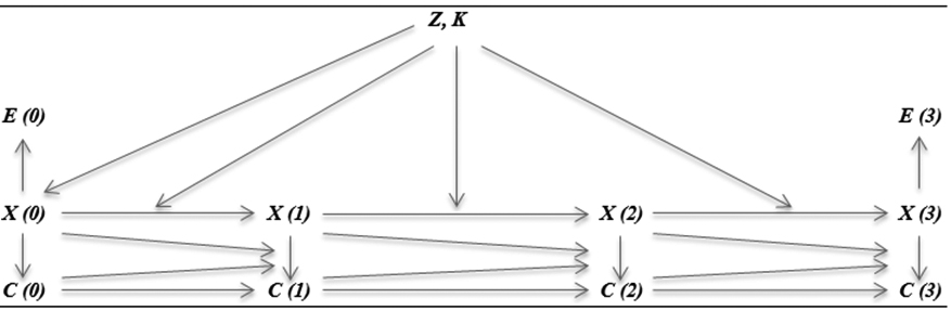

In this mixture HMM, the joint probability of following a particular observed path can be expressed as follows:5

$\displaystyle P(C_{i}=c_{i},E_{i}=e_{i})=\sum^{L}_{x_{0}=1}\sum^{L}_{x_{1}=1}{% \dots}\sum^{L}_{x_{T}=1}$ $\displaystyle P(X_{i0}=x_{0})\prod^{T}_{t=1}P(X_{it}=x_{t}|X_{i(t-1)}=x_{t-1})$ $\displaystyle\prod^{T}_{t=0}P(C_{it}=c_{t}|X_{it}=x_{t})\prod^{T}_{t=0}P(E_{it% }=e_{t}|$ $\displaystyle X_{it}=x_{t})^{{\delta}_{it}}$ (5)

Where $P(X_{i0}=x_{0})$ and $P(X_{it}=x_{t}|X_{i(t-1)}=x_{t-1})$ denote the latent initial state probabilities and (time-homogenous) transition probabilities, respectively. $P(C_{it}=c_{t}|X_{it}=x_{t})$ and $P(E_{it}=e_{t}|X_{it}=x_{t})$ denote the measurement/classification error probabilities for the register and survey data and retain the ICE assumption. The indicator ${\delta}_{it}$ accounts for the fact that the survey observations are only available for every third month and so ${\delta}_{it}=1$ for those months when the LFS took place and ${\delta}_{it}=0$ for those when it did not; $L$ represents the categories of $X$ and $Y$ – $\{$ permanent, temporary, other $\}$ – and runs from 1 to 3; $i$ denotes the individual and runs from 1 to N, while $t$ represents time and runs from 1 to 15.6 We used this model to estimate the transition rates from temporary to permanent employment in the absence and in the presence of linkage error, which we simulated into the original dataset. The difference between the obtained transition rates estimates the bias introduced by linkage error. For further details on the simulation setup see Section 4.1 and [39].

2.2.2 Feasibility of parameter re-use

In the second operation that we examine, we studied the feasibility of using the same error parameter estimates as a correction factor for a number of years, when no change in the data collection occurred. In doing so, we used our “baseline” model (Model C).

This model, which is illustrated in Fig. 2, takes the following form:

$\displaystyle P(C_{i}=c_{i},E_{i}=e_{i}|Z_{i})=\sum^{L}_{k=1}\sum^{L}_{x_{0}=1% }\sum^{L}_{x_{1}=1}{\dots}$ $\displaystyle\sum^{L}_{x_{T}=1}\pi_{k}P(X_{i0}=x_{0}|Z_{i},k)\prod^{T}_{t=1}P(% X_{it}=x_{t}|$ $\displaystyle X_{i(t-1)}=x_{t-1},Z_{i},k)P(C_{i0}=c_{0}|X_{i0}=x_{0})$ $\displaystyle\prod^{T}_{t=1}P(C_{it}=c_{t}|X_{it}=x_{t},X_{i(t-1)}=x_{t-1},$ $\displaystyle C_{i(t-1)}=c_{t-1})\prod^{T}_{t=0}P(E_{it}=e_{t}|$ $\displaystyle X_{it}=x_{t})^{{\delta}_{it}}$ (6)

This specification can be seen as an extension of the one used for the linkage error sensitivity analysis, which allows modelling more realistic scenarios. We extended the model of Eq. (2.2.1) by first relaxing the homogeneity assumption for both the latent initial state probabilities – $P(X_{i0}=x_{0}|Z_{i},k)$ – and the latent transition probabilities – $P(X_{it}=x_{t}|X_{i(t-1)}=x_{t-1},Z_{i},k,t)$ . More specifically, these probabilities are allowed to depend on observed characteristics, i.e. age, gender, education level and ethnicity, which are denoted by $Z_{i}$ . Moreover, the latent initial state and transition probabilities are also corrected for unobserved heterogeneity using a non-parametric method. Namely, it is assumed that individuals belong to $K$ different Markov chains that are represented by time invariant latent classes; $\pi_{k}$ denotes the probability of belonging to a latent class $k$ . Finally, the latent transition probabilities are also assumed to be time-heterogenous and specifically to depend on $t$ and $t^{2}$ .

Second, the ICE assumption is relaxed for the register data and the error probability depends on the lagged observed and lagged true contract type. Following the approach of [33], rather than estimating all corresponding error probabilities, we use a restricted model and focus on the probabilities of repeating the same error. In doing so, we define a logit model for the probability of making an error in the register data – $P(C_{it}=c_{t}|X_{it}=x_{t},X_{i(t-1)}=x_{t-1},C_{i(t-1)}=c_{t-1})$ – which takes the form of $\alpha_{c_{t},x_{t}}+\beta_{c_{t},c_{t-1},x_{t},x_{t-1}}$ . Here, $\alpha_{1_{c_{t},x_{t}}}$ represents the random component of the error, which does not violate the ICE assumption, and $\beta_{c_{t},c_{t-1},x_{t},x_{t-1}}$ represents the systematic (autocorrelated) component of the error which violates this assumption. $\beta_{1_{c_{t},c_{t-1},x_{t},x_{t-1}}}$ is a free parameter if $c_{t}=c_{t-1}\neq x_{t}=x_{t-1}$ (i.e. the same error is repeated for two consecutive months) and is equals to 0 otherwise.

Finally, the measurement error probabilities for the survey data – $P(E_{it}=e_{t}|X_{it}=x_{t})^{\delta_{it}}$ retain the ICE assumption. As in the previous model, $L=\{\textit{perm},\textit{temp},\textit{other}\}$ , $i=1,\ldots,N$ , $t=1,\ldots,15$ and ${\delta}_{it}$ equals 1 if the survey information is available for a given month and 0 if it is missing.

The model used when investigating whether parameter estimates can be carried forward when a change in the interviewing regime takes place is an extension of aforementioned specification (i.e. Model C) that allows for systematic/autocorrelated error in the survey data as well. This extension, which relaxes the ICE assumption for the survey data, is necessary to investigate whether switching an interviewing regime affects the systematic component of the error. It is important to note that this specification continues to account for observed heterogeneity ( $Z_{i}$ ) but, unlike the one in Eq. (2.2.2), it does not account for unobserved heterogeneity by using latent class memberships ( ${\pi}_{k}$ ). This is done to assure that the model specification is not too complex and does not lead to convergence issues. What is more, unlike in the previous models, we only used data from the months in which the (quarterly) survey took place and, therefore, $t$ runs from 1 to 5.

This model can be formalized as follows:

$\displaystyle P(C_{i}=c_{i},E_{i}=e_{i}|Z_{i},W_{i})=\sum^{L}_{x_{0}=1}\sum^{L% }_{x_{1}=1}{\dots}$ $\displaystyle\sum^{L}_{x_{T}=1}P(X_{i0}=x_{0}|Z_{i})\prod^{T}_{t=1}P(X_{it}=x_% {t}|$ $\displaystyle X_{i(t-1)}=x_{t-1},Z_{i})P(C_{i0}=c_{0}|X_{i0}=x_{0})$ $\displaystyle\prod^{T}_{t=1}P(C_{it}=c_{t}|X_{it}=x_{t},X_{i(t-1)}=x_{t-1},$ $\displaystyle C_{i(t-1)}=c_{t-1})P(E_{i0}=e_{0}|X_{i0}=x_{0})$ $\displaystyle\prod^{T}_{t=1}P(E_{it}=e_{t}|X_{it}=x_{t},X_{i(t-1)}=x_{t-1},$ $\displaystyle E_{i(t-1)}=e_{t-1},W_{i})$ (7)

where the (latent) initial state probabilities and transition rates – $P(X_{i0}=x_{0}|Z_{i0})$ and $P(X_{it}=x_{t}|X_{i(t-1)}\linebreak=x_{t-1}|Z_{it},t)$ – depend on observed individual-level heterogeneity $Z_{i}$ (i.e. the covariates education, gender and ethnicity) and the latent transitions also depend on time (i.e. are time-heterogeneous). We relax the ICE assumption and model the presence of systematic error in the measurement error probabilities of both the ER and the LFS – $P(C_{it}=c_{t}|X_{it}=x_{t},X_{i(t-1)}=x_{t-1},C_{i(t-1)}=c_{t-1})$ and $P(E_{it}=e_{t}|X_{it}=x_{t},X_{i(t-1)}=x_{t-1},E_{i(t-1)}=e_{t-1},W_{i})$ . For the register data, the ICE assumption is relaxed in the exact same manner as in the previous model (see Eq. (2.2.2)). In the LFS, similarly to the register data, we allowed the error probabilities to depend on the lagged true contract – $X_{i(t-1)}$ – and the lagged observed contract – $E_{i(t-1)}$ . Additionally, to compare the error levels under DI and INDI, we allow the survey error probabilities to also depend on the covariate $W_{i}$ , which denotes the interviewing regime used and can take 3 values (for further details see Section 4.2.2):

0 (ref. category) INDI was used, but had the interviewing regime not been changed, DI would have been used;

1 INDI was used and would have been used regardless of the interviewing regime change;

2 DI was used.

In our analysis, we focused on comparing the error levels under DI to those where DI would have been used had it not been abolished (i.e. category 2 vs. 0). In doing so, we used a model specification that allows for random error in all cases, but that only allows for systematic error in situations where the errors in the survey data are assumed to be a consequence of cognitive processes. Specifically, the parameters of the systematic error components are freed when the same error can be repeated due to DI – i.e. when $E_{it}\linebreak=E_{i(t{-}{1})}=\textit{temp}\neq X_{it}=X_{i(t{-}{1})}=\{% \textit{perm},\textit{other}\}$ – or when DI might cause spurious stability. That is, in a situation where an individual correctly reports having a temporary contract in $t-1$ , then experiences a true transition between $t-1$ and $t$ but erroneously confirms in t that she/he is still employed on a temporary basis – i.e. when $E_{it}=E_{i(t{-}{1})}=\textit{temp}$ and $X_{it}=\textit{temp}\neq X_{i(t{-}{1})}=\{\textit{perm},\textit{other}\}$ .

For the LFS data, the log-linear error parameters, corresponding to $P(E_{it}=e_{t}|X_{it}=x_{t},X_{i(t-1)}=x_{t-1},E_{i(t-1)}=e_{t-1},W_{i})$ , take the following form $\alpha_{e_{t},x_{t}}+\beta_{e_{t},e_{t-1},x_{t},x_{t-1}}+\alpha_{2_{e_{t},x_{t% },w}}+\beta_{2_{e_{t},e_{t-1},x_{t},x_{t-1},w}}$ . In this specification, the term $\alpha_{{e_{t},x_{t}}}+\alpha_{2e_{t},x_{t},w}$ represents the random component of the error, i.e. it refers to errors that occur in accordance with the ICE assumption. Here, $\alpha_{{e_{t},x_{t}}}$ can be interpreted as the “baseline” probability of a random error occurring and $\alpha_{2_{e_{t},x_{t},w}}$ can be interpreted as the coefficient indicating how different interviewing regimes (DI, INDI, would have had DI) decrease/increase the probability of obtaining random error. The term $\beta_{e_{t},e_{t-1},x_{t},x_{t-1}}+\beta_{2_{e_{t},e_{t-1},x_{t},x_{t-1},w}}$ represents the systematic component of the error, i.e. it refers to an autocorrelated error that violates the ICE assumption. Again, the first part of this expression – $\beta_{{e_{t},e_{t-1},x_{t},x_{t-1}}}$ – corresponds to the “baseline” probability of having systematic error and the second part $\beta_{2_{e_{t},e_{t-1},x_{t},x_{t-1},w}}$ – indicates how different interviewing regimes affect this probability. As mentioned above, $t$ runs from 1 to 5 and as in the previous models $L=\{\textit{perm},\textit{temp},\textit{other}\}$ and $i=1,{\dots},N$ .

All models were estimated using the Latent GOLD software [44]. The parameters are obtained using the forward-backward or Baum-Welch algorithm, which is a variant of the well-known Expectation-Maximization (EM) algorithm [45, 46]. In the E-step, the algorithm estimates the posterior probability – $P(X|Y)$ – by combining the forward and backward recursions. In the forward step, the probability of arriving at a specific state at time $t$ is calculated based on the states that occurred up to (and including) $t-1$ ; in the backward step, this probability is calculated based on the states occurring from $t+1$ onwards. In the M-step, the algorithm computes the model parameters by summing over the states at each time point and weighting the sum by the posterior probabilities. The E- and M-steps are iterated until convergence is reached. In our models all missing values are treated as missing at random (MAR).

3. Data

Our analyses make use of a linked dataset with information coming from the Dutch Labour Force Survey (LFS) and from the Employment Register (ER). As reported by Statistics Netherlands, the linkage effectiveness, that is, the percentage of survey records linked to the ER, is approximately 97%. In our analyses, we assumed the dataset to be linkage-error-free.

The LFS is a sample survey that primarily provides information on labour market participation. The target population consists of individuals aged 15 and older who reside in the Netherlands and are part of the labour force; the information is collected at both the individual and household level. As of the last quarter of 1999 the survey is a rotating trimonthly panel survey, consisting of five waves.7 The survey suffers from non-negligible non-response and attrition rates, which are likely to lead to selectivity issues. To correct for this to the extent possible given data availability, we included a number of covariates in our models.

The ER is an administrative dataset that is managed by the Dutch Employee Insurance Agency (UWV in Dutch). The dataset contains monthly information on wages, benefits, and labour relations for all insured employees in the Netherlands. While the ER combines information from various sources, the core information is the one delivered on a monthly basis by the employers to the Dutch Tax Authorities.8

The sample used for the linkage analysis and parameter re-use analysis when no change in the data collection occurs, consists of 8,886 LFS respondents (aged 25 to 55) who were interviewed for the LFS for the first time in the first trimester of 2009. For each individual included in the sample, the dataset contains information for a period of 15 months resulting in a total of 133,290 observations, wherein the variables coming from the ER data are available on a monthly basis and those from the LFS are observed every 3 months.

The sample used in the parameter re-use analysis when a change in the interviewing process occurred consists of 86,075 LFS respondents (aged 25 to 55) who first participated in the survey either in 2009 (DI in place) or 2010 (DI abolished). It contains quarterly information on each individual for 5 time points, leading to a total sample size of 430,375 observations.

The main variable of interest in our analyses is the individual’s contract type for her/his main job. The contract type can take on three distinct and mutually exclusive values: “permanent contract” (i.e. a contract for an unlimited duration of time), “temporary contract” (i.e. a contract for a limited duration of time) and other, which includes all other alternatives, e.g. self-employment, unemployment, unpaid employment, and full-time education. While both the LFS and ER include a more detailed breakdown of the individual’s contract type, we collapsed these values into the three above mentioned broad categories to prevent a situation whereby any inconsistencies in the data are the result of differences in the underlying concepts.9 While it is still possible that some inconsistencies between the two data sources persist, the constructed categories have largely the same meaning in the survey and register data and, thus, any remaining discrepancies can be considered negligible.

Table 2, which is based on the analysis conducted in [34], provides a cross-tabulation of the contract variable according to the survey and register data for the sample that includes respondents whose first wave of the LFS took place in the first trimester of 2009. The results presented in Table 2 show that there are large discrepancies between the two data sources for individuals holding temporary contracts; the differences in terms of permanent and other types of contract are less substantial. As both sources were subject to editing and the definitions of contract types were aligned, the inconsistencies are (predominantly) a consequence of measurement error.

Table 2
Cross-tabulation of contract type according to the survey and register data

Register	Permanent	Temporary	Other	Total	Cases
	Survey
Permanent	0.934	0.052	0.015	1.000	21,840
Temporary	0.517	0.441	0.043	1.000	5,347
Other	0.060	0.059	0.881	1.000	8,411
Total	0.665	0.112	0.224	1.000	35,598
Cases	23,654	3,983	7,961	35,598	–

Note: The frequency distributions are calculated for all observations in the sample which are non-missing for both the LFS and ER.

4. Results

4.1 Sensitivity of the extended HMM to linkage error

The first challenge related to the application of HMMs is to investigate their sensitivity to linkage error. As linking data sources at the micro level is necessary to be able to apply multiple-indicator HMMs that allow for the reconciliation of inconsistent sources, linkage error is potentially a serious threat to these models. Previous research shows that linkage error, if unaccounted for, leads to considerable bias in the parameters of interest [47]. Therefore, in [39] we investigated the sensitivity of the two-indicator HMM to false-positive and false-negative linkage errors. False negatives occur if records of the same person are not linked. False positives occur if records of two different persons are linked [48].

We carried out a simulation study in which we used the linked 2009 LFS and ER data. We assumed this data to be perfectly linked and simulated various levels and types of linkage error within this dataset. We then estimated the transition rates from temporary to permanent employment for the datasets with the simulated error using the model described in Section 2.2.1. The results for the simulated datasets were compared to transition rates obtained using the original sample (without simulated linkage error); the difference between these two approximates the bias introduced by linkage error.

In more detail, in our simulation strategy, we considered low, medium, and high levels of both false-negative and false-positive linkage error – i.e. 5, 10, and 20% – and different types of errors – i.e. random, dependent on age (which is mildly correlated with the model estimates), and dependent on whether a transition from temporary to permanent employment occurred according to the register data (which is highly correlated with the model estimates).10 For false-positive error we also considered scenarios wherein individuals are mislinked randomly and wherein similar individuals (according to their age, gender, education level and ethnicity) are mislinked.

Table 3
Simulation results- the biasing effects of all false-negative and false-positive linkage error conditions (in %)

Error type	Condition: The probability of being mislinked	Overall error (approx.)	High exclusion probability	Low exclusion probability	Temporary to permanent transition rate
					Transition rate	Absolute bias	Relative bias
No error	Original HMM	0	–	–	6.9	–	–
False-negative	Depends on age	5	15	1	6.6	0.3	4.60
		10	30	1	6.7	0.2	3.20
		20	70	1	6.6	0.3	3.80
	Depends on transition	5	15	5	6.2	0.7	10.60
		10	34	9	5.2	1.7	25.00
		20	90	17	1.1	5.8	84.30
False-positive; mislinkage	Random	5	–	–	6.9	0	0.05
with random donor		10	–	–	6.9	0	0.26
		20	–	–	6.8	0.1	0.95
	Depends on age	5	15	1	6.9	0	0.26
		10	30	1	6.8	0.1	1.20
		20	70	1	6.7	0.2	2.56
	Depends on transition	5	15	5	6.4	0.5	7.82
		10	34	9	5.5	1.4	20.67
		20	90	17	2.4	4.5	64.61
False-positive; mislinkage	Random	5	–	–	6.7	0.2	3.15
with similar donor		10	–	–	6.7	0.2	3.18
		20	–	–	6.6	0.3	4.90
	Depends on transition	5	15	5	6.1	0.8	11.52
		10	34	9	5.1	1.8	26.62
		20	90	17	1.2	5.7	82.59

The simulations were designed in the following way. In the first step, we identified younger individuals or individuals who had at least one three-monthly transition from temporary to permanent employment recorded in the register data; this step was omitted for the random mislinkage conditions. Next, in each condition we assigned one of two exclusion/mislinkage probabilities to each individual in our sample. We assigned a “high” probability to the individuals identified in the first step and a “low” probability to all remaining individuals. We set the exclusion/mislinkage probabilities to be such that (i) the overall linkage error rates remained 5, 10, and 20 %; and that (ii) conditions with higher linkage rates are also characterized by greater differences between the low and high probabilities. In the random mislinkage conditions, all individuals were assigned the same probability, which was equal to the corresponding linkage error rate. To illustrate, for the conditions where the exclusion/mislinkage probability depended on age, we set the high threshold (i.e. that of individuals aged 25 to 34) to 0.15, 0.30, and 0.70 when the overall exclusion rate was 5, 10 and 20 % respectively; the low threshold (i.e. that of individuals aged 35 to 54) remained at 0.01 in all three cases.

Then, given the assigned probabilities, we selected individuals for exclusion/mislinkage at random. In doing so, for each individual in the sample, we drew a random number from a standard uniform distribution – $U_{i}\sim U(0,1)$ – and if the drawn number was smaller or equal to the assigned probability $p-(U_{i}\leqslant p)$ – we excluded the individual from the sample or mislinked them. When mislinking individuals, we assigned the selected individuals to a donor, who was either chosen at random or based on similarity w.r.t. age, gender, nationality, and education, and replaced the individuals contract type according to the register data with that of the donor.

The results of the simulations are summarized in Table 3. They show that the biasing effects of both false-negative and false-positive linkage errors are in most cases negligible. The resulting bias is substantial and varies from 20 to 80% only when the exclusion/ mislinkage probability depends on a covariate (very) strongly correlated with the model outcomes, i.e. transitioning from temporary to a permanent contract in the register data, and when the overall level of the error is 10 or 20%. For all random and age- dependent conditions, the relative bias is below 5%. When the linkage error rate amounts to 5% and is transition-dependent, the bias is either below 10% (for one condition) or slightly above 10% (for two conditions). Thus, it can be concluded that the model estimates of the extended HMM are primarily sensitive to linkage error in situations where the error probability (strongly) depends on a covariate that is very highly correlated with the model estimates. In situations that are less extreme, the bias is relatively small and can be considered negligible.

Figure 3.

Level of measurement error by type and level of mislinkage.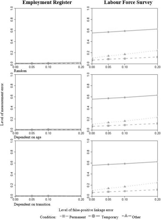

Table 4

Measurement error probabilities in the survey and register data

Note: standard errors are always smaller than 0.0001.
Survey data
	Conducting analysis “from scratch”			Using Pavlopoulos and Vermunt (2015) error parameter estimates
	Observed type of contract in $t$			Observed type of contract in $t$
Latent type of contract in $t$	Permanent	Temporary	Other	Permanent	Temporary	Other
Permanent	0.996	0.003	0.002	0.998	0.001	0.002
Temporary	0.090	0.878	0.033	0.125	0.832	0.042
Other	0.011	0.006	0.984	0.004	0.005	0.991
Note: standard errors are always smaller than 0.0001.
Register data
	Conducting analysis “from scratch”			Using Pavlopoulos and Vermunt (2015) error parameter estimates
	Observed type of contract in $t$			Observed type of contract in $t$
Latent type of contract in $t$	Permanent	Temporary	Other	Permanent	Temporary	Other
Permanent	0.877	0.106	0.017	0.888	0.081	0.031
Temporary	0.247	0.635	0.118	0.237	0.684	0.079
Other	0.033	0.013	0.954	0.032	0.017	0.951

The reported findings are rather intuitive for false-negative linkage error, which is essentially missingness not at random.11 They are, however, rather surprising for false-positive linkage error, as even relatively low levels of this type of error are expected to (heavily) bias estimates [49, 50]. A closer look at the levels of measurement error for the different mislinkage scenarios, which are displayed in Fig. 3, provides some explanation for these puzzling findings. That is, the simulation results suggest that measurement error and false-positive linkage error move in tandem. Put differently, higher levels of false-positive linkage error lead to higher levels of measurement error. This implies that under many circumstances false-positive linkage error is simply another source of measurement error that is absorbed by the HMM and, as this error is corrected for, it does not significantly bias the structural parameter estimates. It is worthwhile noting that this pattern is particularly visible in the LFS data and less so in the ER data, as the simplified HMM used in this analysis does not account for autocorrelation of the error in the ER data. As measurement error in the register is mainly systematic, the model fails to capture the error altogether and assumes the data in this case to be almost completely free of error.

4.2 The feasibility of parameter re-use

The second main challenge associated with the application of (extended) hidden Markov models in official statistics production is their complicated nature. Namely, utilizing HMMs in this domain is very time consuming and therefore expensive, as it requires NSIs to perform record linkage followed by model re-estimation for each new time period. While theoretically it is possible to run the analysis periodically and use the obtained error parameter estimates as a correction factor for a number of years, this practice is conditioned on the assumption that the size and structure of the measurement error parameters for the survey and register data are constant for the relevant time period.

Carrying forward estimates of measurement error may cause bias if the size and/or structure of the error either gradually change over time or change due to (major) modifications in the data collection process. Gradual changes can be associated, for instance, with over-time improvements in data quality resulting from survey interviewers getting accustomed to a questionnaire when using it for numerous consecutive waves. Furthermore, companies providing register data may get used to the software that is utilized for this purpose and as a result submit more accurate data. Such gradual changes can also be associated with small, seemingly trivial alterations to data collection processes which are not properly registered and documented, such alterations can include an update of a data-collection software for register data and the hiring of new interviewers for survey data. Major changes, on the other hand, are usually well documented by NSIs and have the potential to substantially influence the size and/or structure of the error going forward. Such changes include e.g. altering the sample design from address to person based, switching between different interviewing techniques, e.g. shifting from dependent to independent interviewing, or switching interviewing modes, e.g. shifting from face-to-face to telephone or internet survey [51]. Therefore, in [34] we looked at whether parameter estimates can be carried forward when no significant change occurs and in [41] we examined whether this can be done when a major change in the interviewing regime occurs.

Table 5
Observed and latent distribution of contract type and latent transitions from temporary to permanent contracts – $P(X_{it}=x_{t}|X_{t(t-1)}=x_{t-1},Z_{t},k,t)$

	Observed type of contract		Latent type of contract
	Survey	Register	Conducting analysis “from scratch”	Using Pavlopoulos and Vermunt (2015) error parameter estimates
Permanent	0.653	0.585	0.611	0.613
Temporary	0.110	0.151	0.128	0.131
Other	0.237	0.264	0.261	0.257
Temp to perm transition rate	0.058	0.073	0.017	0.016
Cases	36,321	130,671	133,290	133,290

Note: standard errors are always smaller than 0.0001.

4.2.1 No changes in the data collection process

In [34], we studied the feasibility of re-using existing error parameter estimates from [33] in order to estimate the structural parameters (i.e. the true contract type distributions and transitions between these contract types) with more recent data. In doing so, we applied the extended HMM used by [33] to linked LFS and ER data from 2009. Then, we repeated the analysis for the same sample while fixing the measurement error parameters to those obtained by [33] when analyzing 2007 data from the same data sources. Having done that, we compared the results of the two analyses. It is worthwhile noting that, as described in Section 2.1, our analysis also tested the model fit of various model specifications to make sure that the same specification can be used to correct for measurement error for a certain period of time.

Table 4 displays the size of the measurement error in the 2009 survey and register data estimated, first by using the “full” approach (i.e. applying the extended HMMs to the 2009 data) and, second, by fixing the error parameters to those obtained from [33]. When estimating the error, we used the posterior probabilities of having a specific type of latent contract in each month for each individual – $P(X_{it}=x_{it}|Y_{it}=y_{it},\ Z_{i}=z_{i})$ . Overall, the results are extremely similar in both analyses and exhibit the same trends with regards to the size of the measurement error, suggesting that the error is stable over the time period studied. As mentioned above, this allows us to correct for measurement error without having to undertake the full HMM analysis.

Table 5 provides the observed and latent distributions for different contract types and the 3-monthly transition rates from temporary to permanent employment. The results of the “full” analysis are almost identical to those using the fixed error parameters and show that the latent probability of belonging to a certain state always lies between the observed probabilities according to the two data sources. The transition rates, on the other hand, are shown to be (significantly) lower than what is suggested by either the survey or register data. More specifically, the average 3-monthly transition rate from temporary to permanent employment in 2009 (i.e. the main quantity of interest) amounts to almost 6% according to the survey data and just over 7% according to the register data. According to both of our analyses, however, the error-corrected transition rate is equal to less than 2%; more specifically, it amounts to 1.6% when the analysis is run “from scratch” and to 1.7% when the error parameters are fixed to those obtained using 2007 data.

4.2.2 A major change in the data collection process

While our results suggest that error parameter estimates can be re-used in the absence of major changes in the data collection process (as the error appears stable over time), it may not be the case if NSI’s do implement a significant change in the time period under consideration. Any substantial modifications in the way data are collected might significantly impact the structure and/or size of measurement error. This in turn can lead to a situation whereby the re-used parameter estimates are based on an incorrect model specification and/or do not reflect the correct magnitude of the error in the data. Such misspecifications are likely to lead to biased estimates. We examine the implications of such a scenario, using as an illustrative example the switch from dependent interviewing (DI) to standard, independent interviewing (INDI) in the Dutch LFS.

Figure 4.

Interviewing setup for the survey question on employment contract type.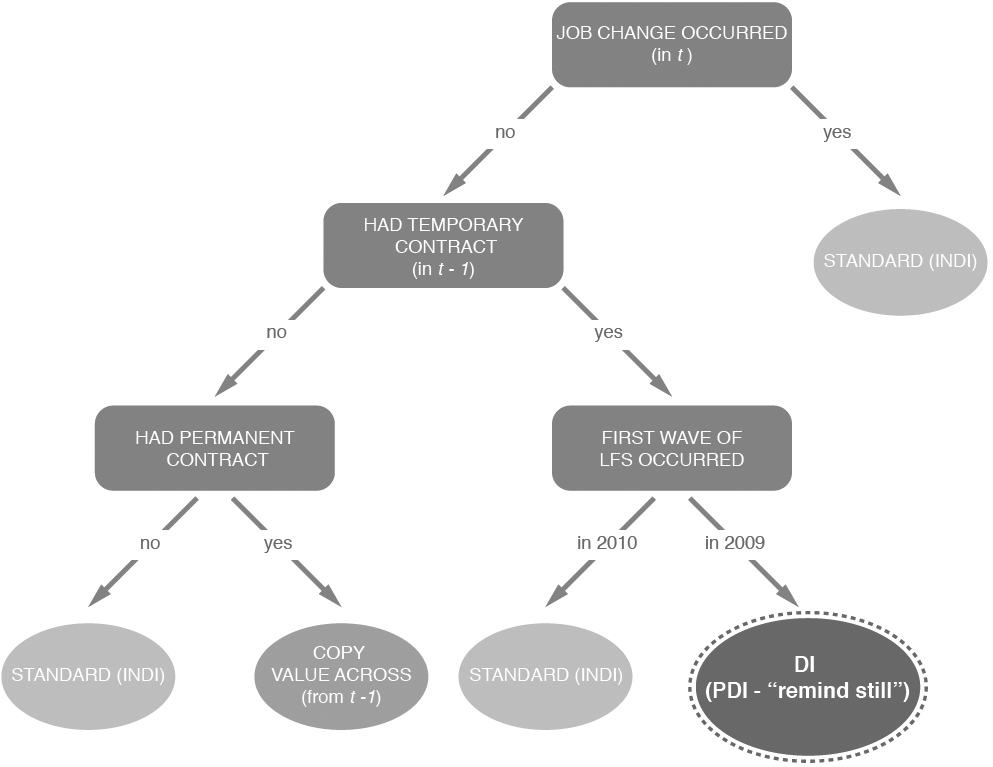

DI, and more specifically the “remind, still” style of proactive DI (PDI), was in use in the LFS until the end of 2009; at the beginning of 2010 it was replaced by standard INDI. Survey respondents who first participated in the LFS before the end of 2009 were asked about their employment contract using DI if they met two conditions: (i) they indicated in the previous wave that they had a temporary contract and (ii) they reported no job change since the previous wave. Respondents who were subject to DI were asked the following question regarding their contract type: “Last time you had a temporary contract. Is this still the case?” Individuals who (i) first participated in the LFS after the end of 2009; or (ii) first participated before the end of 2009 but either changed jobs or reported having other type of contract in the previous wave (and no job change) were asked the question using INDI: “Do you currently have a permanent contract?”. The interviewing setup is summarized in the flowchart of Fig. 4. To restate and as shown in Fig. 4:

individuals who experienced a job change in $t$ were subject to INDI both in 2009 and 2010;

individuals who remained in the same job in $t$ and reported having a permanent contract in $t-1$ were not asked the contract question altogether and their answer from $t-1$ was copied forward;

individuals who remained in the same job in $t$ and reported having other type contract in $t-1$ were subject to INDI;

individuals who remained in the same job in $t$ and reported having temporary contract in $t-1$ were subject to DI if they first took the LFS in 2009 and subject to INDI if they first participated in the survey in 2010.

When investigating the effect of transitioning from DI to INDI on both the random and systematic components of the measurement error in the LFS, we used the extended model described in the empirical model section (Section 2.2.2.) Our results, which are summarized in Table 6, are in line with those of previous studies [52, 53, 54] and confirm that DI lowers the incidence of random measurement error. That is, the log-linear parameter estimates corresponding to the probability of misreporting true temporary contract as permanent or other are significantly lower for DI than INDI $({{\alpha}}_{{\textit{perm}}_{t},{\textit{temp}}_{t,2}}=-0.64,p=0.00$ and ${{\alpha}}_{{\textit{other}}_{t},{\textit{temp}}_{t,2}}=-0.47,p=0.02$ , respectively).

On the other hand, unlike what some studies suggest [55, 56], in our case DI does not seem to have an effect on the systematic component of the error. Namely, the log-linear parameter estimates of repeating the same error or of underreporting true change for DI and INDI are not significantly different from each other. It is worthwhile mentioning that our results also suggest that the survey data suffers from autocorrelated errors regardless of the interviewing techniques used; namely, even when the question is asked using standard INDI. More specifically, the “baseline” log-linear parameter estimates of repeating an error confirm that there is an extremely high probability of an LFS respondent repeating the same error if no true change occurred, regardless of the interviewing regime (i.e. $\beta=13.6,p=0.03$ when ${\textit{LFS}}_{t}={\textit{LFS}}_{t-1}=\textit{temp}\neq{\textit{TRUE}}_{t}={% \textit{TRUE}}_{t-1}=\textit{perm}$ and $\beta=19.5,p=0.03$ when ${\textit{LFS}}_{t}={\textit{LFS}}_{t-1}=\textit{temp}\neq{\textit{TRUE}}_{t}={% \textit{TRUE}}_{t-1}=\textit{other}$ ).

Unlike how we hypothesized, DI also does not seem to increase the probability of obtaining systematic errors related to spurious stability, whereby an individual correctly answered the question in $t-1$ , then experienced a true change but failed to report this at $t$ .

Table 6

Random and systematic measurement error parameter estimates

Random (whereby the log-linear parameter corresponds to the following term $\alpha_{{e_{t},x_{t}}}+\alpha_{2e_{t},x_{t},w}$ )
When DI was used (ref. cat. INDI)
Observed type of contract in survey	Latent type of contract	Log-linear parameter	S.E.	Sig.
Temporary	Permanent	10.25	12.52	0.41
Permanent	Temporary	$-$ 0.64	0.10	0.00
Other	Temporary	$-$ 0.47	0.20	0.02
Temporary	Other	18.44	17.90	0.30

Systematic (whereby the log-linear parameter corresponds to the following term $\beta_{e_{t},e_{t-1},x_{t},x_{t-1}}+\beta_{2_{e_{t},e_{t-1},x_{t},x_{t-1},w}}$ )
When DI was used (ref. cat. INDI)
Observed type of contract in survey (in $t$ )	Observed type of contract in survey (in $t-1$ )	Latent type of contract (in $t$ )	Latent type of contract (in $t-1$ )	Log-linear parameter	S.E.	Sig.
Temporary	Temporary	Permanent	Permanent	$-$ 9.45	12.53	0.45
Temporary	Temporary	Other	Other	19.43	17.98	0.28
Temporary	Temporary	Permanent	Temporary	2.23	8.37	0.79
Temporary	Temporary	Other	Temporary	23.03	17.9	0.69
When INDI was used (“baseline” probabilities)
Temporary	Temporary	Permanent	Permanent	13.6	6.40	0.03
Temporary	Temporary	Other	Other	19.5	9.11	0.03

More specifically, the parameter estimates corresponding to a situation whereby an individual falsely reported having a temporary contract in $t-1$ and $t$ while in fact in both time points he/she held either a permanent or other type of contract are not statistically significant ( ${\beta}_{\textit{temp}_{t},\textit{temp}_{{t-1}},{\textit{perm}}_{t},{\textit{% perm}}_{t-1},2}=-9.45,p=0.45$ and ${\beta}_{\textit{temp}_{t},{\textit{temp}}_{{t-1}},{\textit{other}}_{{t}},{% \textit{other}}_{t-1},2}=19.43,p=0.28$ , respectively). The probabilities of correctly reporting a temporary contract in $t-1$ , but then experiencing a true transition to either permanent or temporary employment in $t$ and failing to report it also seem unaffected by PDI ( ${{\beta}}_{\textit{temp}_{t},{\textit{temp}}_{{t-1}},{\textit{perm}}_{{t}},{% \textit{temp}}_{{t-1}},2}=2.23,p=0.79$ and ${{\beta}}_{\textit{temp}_{t},{\textit{temp}}_{{t-1}},{\textit{other}}_{t},{% \textit{temp}}_{{t-1}},2}=23.03,p=0.69$ , respectively). The high coefficient estimates observed in Table 6 are a consequence of either extremely low or high corresponding “baseline” probabilities (i.e. under INDI). In these cases, even a small increase in the probabilities in absolute terms can have a substantial relative effect.

Overall, our findings suggest that while this particular change in the survey data collection process did not impact the structure of the error, and therefore does not require a different model specification, the size of the (random) error was significantly affected. Therefore, it is advisable to re-run the analysis “from scratch” in this case as the error parameter estimates obtained for pre-change data do not reflect the true level of error for the post-change data.

5. Conclusions and discussion

NSIs often retrieve information on one phenomenon from different data sources. However, due to measurement and specification errors, those sources often provide inconsistent (or incoherent) estimates. In this paper we focused on measurement error as specification error is negligible in our application. While NSIs currently apply various techniques to deal with this problem, such as weighting, or micro- and macro-integration, we propose a different and arguably superior method, which allows for the reconciliation of inconsistent categorical, longitudinal data sources, and relies on the use of HMMs.

HMMs are an attractive method that allows for the correction of measurement error in categorical, longitudinal data as they do not require the availability of error-free, benchmarking source and they allow for the correction of error in multiple sources simultaneously. However, the incorporation of HMMs in the production of official statistics faces two main challenges. Namely, to reconcile two or more inconsistent sources simultaneously and produce one set of consistent estimates, the use of multiple-indicator HMMs is required. Such extended versions of the models require linking data on the micro level, a procedure which might result in linkage error. As linkage error has potentially strong biasing effects, the sensitivity of the HMM (structural) estimates to this type of error needs to be investigated. What is more, the procedures involved in the application of such extended models in the production of official statistics are complicated, time-consuming and, thus, expensive, and they cannot be applied regularly. While it is possible to simplify this process by re-using error parameter estimates from previous time points with more recent data without having to link datasets again and applying the full modelling technique, this procedure relies on the assumption that the size and structure of the error are constant over the time period under consideration. It is, therefore, necessary to verify whether the size and/or structure of measurement error change over a period of several years both in the absence and presence of a major change in the data collection process.

This overview paper examines the feasibility of using HMMs to reconcile inconsistent data sources and produce consistent estimates given the two issues highlighted above. Our results are overall very promising and suggest that HMMs can be used in the production of official statistics as the HMMs estimates are largely robust to linkage error and the size and structure of the error remain stable over time, unless a major change in the data collection occurs, such as a switch in the interviewing regime.

In more detail, the results of our simulation study show that the sensitivity of the method to linkage error is low. Only scenarios with very high levels of linkage error (around 20%) and where the probability of exclusion or mislinkage is highly correlated with model estimates lead to substantial bias. Such extreme scenarios, however, are rather unlikely to often occur in practice. In our second analysis we show that the size and structure of the error are time-invariant for the period 2007 to 2009. The choice to use 2009 data was motivated by the fact that the period between 2007 and 2009 was characterized by a lack of any major modifications to the data collection process. That is, the results of our second analysis show that reusing error parameters, obtained from an HMM that was estimated on data from 2007, on data from 2009 leads to virtually the same results as running the 2009 analysis “from scratch”. This procedure shares some similarities with the revision strategies used for accounting systems, such as the National Accounts. That is, after a period of e.g. three or five years, the sources, procedures and methods used have to be determined again.12 Likewise, the reuse of error parameters for three or more years should be followed by a revision of the error parameters so they reflect gradual over time changes in the magnitude and/or structure of the error in the sources as well as any changes that occurred in the data collection procedures.

On the other hand, our final analysis implies that the size and/or structure of the error are affected when an important change in the data collection process occurs, as the transition from DI to INDI significantly affects the size of the random component of the error. Therefore, any substantial alterations to the process by which data are collected should be followed by a complete re-estimation of the HMM from the new data. This implies that the proposed method can still be rather expensive, if the data collection process of a survey or the laws and regulations impacting register data quality change frequently. The decision of whether this method should be applied in the production of official statistics depends then on the expected frequency of the aforementioned changes (i.e. the costs involved) and the importance of obtaining consistent and error-corrected variables for the users of official statistics (i.e. the revenues).

Another important factor that should be taken into consideration is that all the models that we refer to use linked data. This implies that, if one of the sources used is much richer than the other (i.e. it contains more individuals and/or more time points per individual), such as is the case with register data compared to survey data, this method will lead to loss of information, as it only uses data available in both sources.13 Moreover, if the survey data are suffering from selective non-response, the estimated measurement error can be biased too. For this reason, NSI’s might prefer using macro-integration or reweighting techniques as these methods use all the data available rather than just a linked subset. Further research should, therefore, look into the possibility of combining the aforementioned methods with hidden Markov modeling. In such a combined method, HMMs could be used to obtain estimates of measurement error from the linked data, while the final corrected (substantive) estimates could be based on all the data available and obtained using macro-integration or reweighting techniques.

Other issues that need to be investigated further, before this method can be put into production, include the consideration of other more complex and therefore more realistic models. This should include specifications that relax the first-order Markov assumption and allow for second and higher order effects in the transitions between true contract types. Furthermore, the assumption of local independence between the data sources should also be tested. While this is not possible to do with only two data sources, adding another data source would enable investigating this. Finally, it is also worthwhile mentioning that our analysis did not use weights. While in our analysis the inclusion of sampling weights did not significantly affect the results (and therefore we decided to exclude them), this might not be the case in other applications, in particular when the weights vary substantially across respondents. Therefore, it is worth investigating the impact of including weights in a different setting wherein they are expected to have a stronger effect.

Footnotes

Please note that in the language of Official Statistics the term ‘coherent’ is often used instead of ‘consistent’ when referring to estimates that agree.

It is important to note that, extended HMMs can handle data with missing values whereby for some time points only one indicator is available.

Thus, the requirement of linked data implies that the HMM method cannot be used to consolidate inconsistent data sources (with overlapping variables) if these sources have almost no units in common, such as two (disjunct) samples.

In more detail, we opted for simple model specification that will assure the feasibility of the simulation study (rather than a complex, more realistic model that takes significantly longer to converge).

The reparameterization of the model probabilities using multinomial logistic equations, follows [].

While in our analysis we used data from January 2009 until May 2010 which corresponds to an overall period of 17 months, the data available per individual covers a 15-month period. The discrepancy is a result of the fact that our sample consists of individuals who first participated in the LFS either in January, February or March 2009 and were subsequently followed for a period of 15 months.

http://www.cbs.nl/en-GB/menu/methoden/dataverzameling/dutch -labour-force-survey-characteristics.htm.

https://www.uwv.nl/overuwv/english/about-us-executive-board-organization/detail/organization/data-services.

In the LFS the following categories are classified as a permanent contract: Permanent employees, constant hours and Permanent employees, flexible working hours. Those with a flexible contract are: Temporary employees with a prospect on a permanent contract; Temporary employees, $\geqslant$ 1 year; Temporary employee, $<$ 1 year; Temporary agency worker; On-call worker; Temporary employee, flexible hours. Other: Self-employed and persons without a job. In the ER the following categories are classified as a permanent contract: Employees with a regular job and a permanent contract. Those with a flexible contract are: Employees with a regular job and a temporary contract; Internees; Temporary agency worker with and without a permanent contract; On-call worker with and without a permanent contract. Other: Persons without a job; Managing director and majority shareholder.

In [] we show that age has a moderate, negative effect on the probability of transitioning from temporary to permanent employment; according to the model used for the linkage analysis, more than 99% of all contracts observed in ER are correctly classified and, thus, the transition covariate is very highly correlated with the model estimates.

In the false-negative linkage error conditions, the exclusion probability depends on covariates that are not controlled for in the model. Therefore, the resultant sample has missing data and the missingness is correlated with the model estimates which is equivalent to an MNAR situation.

https://ec.europa.eu/eurostat/web/products-manuals-and-guide lines/-/KS-02-13-269.

While it is possible to apply standard, one-indicator HMMs to each of the sources separately, such a procedure will not lead to the reconciliation of inconsistent sources.

Acknowledgments

The first author acknowledges the contribution of Statistics Netherlands for financing her PhD project and for making the data available for this research. The authors thank the reviewers of the journal, the members of the SILC research group of the Vrije Universiteit Amsterdam as well as Jeroen Pannekoek and the CBS Methodology Advisory Board for reviewing the paper and providing valuable comments and constructive feedback. Finally, the authors also thank Richard Price for both reviewing and editing the paper. This paper is based on .

Appendix I. Weighting on misclassified variables-simulation results

To illustrate that weighting on misclassified variables introduces more bias in the marginal probabilities of other variables (rather than removing it), we conducted a small simulation study. In doing so, we constructed the following true cross table between $X$ (the latent covariate; a multinomial random variable with two categories – ${X=1}$ and ${X=2}$ ) and $Y$ (the target variable; also, a multinomial random variable with two categories – $Y=1$ and ${Y=2}$ ), where $L={{\log}(OR)}=2.60$ :

Table A1

Cross table of true, latent $X$ by $Y$

	${Y}={1}$	${Y}={2}$	Total
$X=1$	0.30	0.20	0.50
$X=2$	0.05	0.45	0.50
Total	0.35	0.65	1

We then defined the following misclassification/ conditional classification probabilities matrix for $X$ where the classification error/measurement error amounts to 0.2 for ${X=1}$ and 0.3 for $X=2$ :

Table A2

Misclassification matrix for $X$ (cross table of observed $X$ by true, latent $X$ )

	$X_{\textit{true}}=1$	$X_{\textit{true}}=2$
${{X}}_{\textit{observed}}={1}$	0.80	0.30
${{X}}_{\textit{observed}}={2}$	0.20	0.70

Combining the two tables allows us to obtain the observed cross table between $X$ and $Y$ (i.e. the cross table between $X_{\textit{observed}}$ , which is the observed/measured value of $X$ that contains classification error, and $Y$ ) which is a mixture over correct and incorrect classifications of $X$ :

Table A3

Cross table of observed $X$ by $Y$

	${{Y}}_{{1}}$	${{Y}}_{{2}}$	Total
${{X}}_{{1},\textit{observed}}$	0.255	0.295	0.55
${{X}}_{{2},\textit{observed}}$	0.095	0.355	0.45
Total	0.35	0.65	1

The log odds ratio calculated based on the observed table is biased and equals to 1.17, as are the observed marginal probabilities for $X$ , which amount to 0.55 and 0.45 rather than 0.5 and 0.5. The observed marginal probabilities for $Y$ , on the other hand, are unaffected by the misclassification error and equal to the true ones (i.e. 0.35 and 0.65).

Next, we calculated weights and defined them as the marginal probabilities of $X$ divided by the observed (misclassified) marginal probabilities:

$\displaystyle W_{i}=\textit{total}_{\textit{true},i}/\textit{total}_{\textit{% observed},i}$

We then applied the obtained weights (i.e. $W_{1}=0.91$ and $W_{2}=1.11$ ) to the observed cross table (Table A.3) and obtained the following (weighted) cross table:

Table A4

Weighted cross table of observed $X$ by $Y$

	${{Y}}_{{1}}$	${{Y}}_{{2}}$	Total
${{X}}_{{1},\textit{observed}}$	0.232	0.268	0.500
${X}_{{2},\textit{observed}}$	0.106	0.394	0.500
Total	0.340	0.660	1

As a result, we removed the bias introduced by classification error from the marginal probabilities of $X$ but introduced bias in the estimates of the marginal probabilities of $Y$ (which were unbiased prior to the weighting). The log odds ratio based on the weighted table is the same as the one based on the unweighted, observed table ( $L=1.17$ ).

References

Bakker

BFM

. Micro-Integration. Method Series. Statistics Netherlands, The Hague. 2011.

var Delden

Pannekoek

Banning

de Boer

. Analysing correspondence between administrative and survey data. Statistical Journal of the IAOS. 2016; 32(4): 569–84.

de Waal

Pannekoek

Scholtus

. Handbook of statistical data editing and imputation. Hoboken (NJ): John Wiley & Sons; 2011.

de Waal

. Obtaining numerically consistent estimates from a mix of administrative data and surveys. Statistical Journal of the IAOS. 2016; 32(2): 231–43.

Guarnera

Varriale

. Estimation from contaminated multi-source data based on latent class models. Statistical Journal of the IAOS. 2016; 32(4): 537–44.

Saris

Gallhofer

. Design, evaluation, and analysis of questionnaires for survey research. Hoboken (NJ): John Wiley & Sons; 2014.

Alwin

. Margins of error: A study of reliability in survey measurement. Vol. 547. Hoboken (NJ): John Wiley & Sons; 2007.

Biemer

. Latent class analysis of survey error. Hoboken (NJ): John Wiley & Sons; 2011.

Sudman

Bradburn

Schwarz

. Thinking about answers: The application of cognitive processes to survey methodology. Psyccritiques. 1997; 42(7): 652.

10.

Tourangeau

Rips

Rasinski

. The psychology of survey response. Cambridge (UK): Cambridge University Press; 2000.

11.

Bakker

. Estimating the validity of administrative variables. Statistica Neerlandica. 2012; 66(1): 8–17.

12.

Oberski

Kirchner

Eckman

Kreuter

. Evaluating the quality of survey and administrative data with generalized multitrait-multimethod models. Journal of the American Statistical Association. 2017; 112(520): 1477–89.

13.

Scholtus

Bakker

van Delden

. Modelling measurement error to estimate bias in administrative and survey variables. Statistics Netherlands. Discussion Paper number: 17, 2015.

14.

Oberski

. Estimating error rates in an administrative register and survey questions using a latent class model. In: Biemer

de Leeuw

Eckman

Edwards

Kreuter

Lyberg

, et al., eds. Total Survey Error in Practice. Hoboken (NJ): John Wiley & Sons; 2017. pp. 339–58.

15.

Huynh

Rupp

Sears

. The assessment of Survey of Income and Program Participation (SIPP) benefit data using longitudinal administrative records. U.S. Department of Commerce U.S. CENSUS BUREAU. Report number: 238, 2002.

16.

Bakker

Daas

. Methodological challenges of register-based research. Statistica Neerlandica. 2012; 66(1): 2–7.

17.

Zhang

. Topics of statistical theory for register-based statistics and data integration. Statistica Neerlandica. 2012; 66(1): 41–63.

18.

Bound

Brown

Mathiowetz

. Measurement error in survey data. In: Heckman

Leamer

, eds. Handbook of econometrics. New York: Elsevier; 2001. pp. 3705–843.

19.

Bolck

Croon

Hagenaars

. Estimating latent structure models with categorical variables: One-step versus three-step estimators. Political Analysis. 2004; 12(1): 3–27.

20.

Pavlopoulos

Muffels

Vermunt

. How real is mobility between low pay, high pay and non-employment? Journal of the Royal Statistical Society: Series A (Statistics in Society). 2012; 175(3): 749–73.

21.

Liu

. Measurement error and its impact on partial correlation and multiple linear regression analyses. American Journal of Epidemiology. 1988; 127(4): 864–74.

22.

de Waal

var Delden

Scholtus

. Multi-source Statistics: Basic Situations and Methods. Statistics Netherlands. Discussion Paper number: 12, 2017.

23.

Särndal

Swensson

Wretman

. Model assisted survey sampling. New York: Springer Science & Business Media; 2003.

24.

Cochran

. Sampling techniques. Hoboken (NJ): John Wiley & Sons; 2007.

25.

Wolter

. Introduction to variance estimation. New York: Springer Science & Business Media; 2007.

26.

Houbiers

. Towards a social statistical database and unified estimates at Statistics Netherlands. Journal of Official Statistics. 2004; 20(1): 55.

27.

Daalmans

. Pushing the boundaries for automated data reconciliation in official statistics [dissertation]. Tilburg: Tilburg University; 2019.

28.

var Rooijen

Bloemendal

Krol

. The added value of micro-integration: Data on laid-off employees. Statistical Journal of the IAOS. 2016; 32(4): 685–92.

29.

Byron

. The estimation of large social account matrices. Journal of the Royal Statistical Society: Series A (General). 1978; 141(3): 359–67.

30.

Denton

. Adjustment of monthly or quarterly series to annual totals: An approach based on quadratic minimization. Journal of the American Statistical Association. 1971; 66(333): 99–102.

31.

Stone

Champernowne

Meade

. The precision of national income estimates. The Review of Economic Studies. 1942; 9(2): 111–25.

32.

Biemer

. An analysis of classification error for the revised current population survey employment questions. Survey Methodology. 2004; 30(2): 127–40.

33.

Pavlopoulos

Vermunt

. Measuring temporary employment. Do survey or register data tell the truth? Survey Methodology. 2015; 41(1): 197–214.

34.

Pankowska

Bakker

Oberski

Pavlopoulos

. Reconciliation of inconsistent data sources by correction for measurement error: The feasibility of parameter re-use. Statistical Journal of the IAOS. 2018; 34(3): 317–29.

35.

Boeschoten

Oberski

De Waal

. Estimating classification errors under edit restrictions in composite survey-register data using multiple imputation latent class modelling (MILC). Journal of Official Statistics. 2017; 33(4): 921–62.

36.

Boeschoten

de Waal

Vermunt

. Estimating the number of serious road injuries per vehicle type in the Netherlands by using multiple imputation of latent classes. Journal of the Royal Statistical Society: Series A (Statistics in Society). 2019; 182(4): 1463–86.

37.

Boeschoten

Oberski

De Waal

38.

Biemer

Bushery

. On the validity of Markov latent class analysis for estimating classification error in labor force data. Survey Methodology. 2000; 26(2): 139–52.

39.

Pankowska

Bakker

BFM

Oberski

Pavlopoulos

. How linkage error affects hidden markov model estimates: A sensitivity analysis. Journal of Survey Statistics and Methodology. 2019; 8(3): 483–512.

40.

Kapteyn

Ypma

. Measurement error and misclassification: A comparison of survey and register data. Journal of Labor Economics. 2007; 25(3): 513–51.

41.

Pankowska

Pavlopoulos

Oberski

Bakker

BFM

. Dependent interviewing: a remedy or a curse for measurement error in surveys? Forthcoming.

42.

Bassi

Hagenaars

Croon

Vermunt

. Estimating true changes when categorical panel data are affected by uncorrelated and correlated classification errors: An application to unemployment data. Sociological Methods & Research. 2000; 29(2): 230–68.

43.

Pavlopoulos

Pankowska

Bakker

Oberski

. Modelling error dependence in categorical longitudinal data. In: Cernat

Sakshaug

, eds. Measurement Error in Longitudinal Data. Oxford (UK): Oxford University Press; Forthcoming.

44.

Vermunt

Magidson

. Technical guide for Latent GOLD 5.0: Basic, advanced, and syntax. Belmont, MA: Statistical Innovations Inc.; 2013.

45.

Vermunt

Tran

Magidson

. Latent class models in longitudinal research. In: Menard

, ed. Handbook of longitudinal research: Design, measurement, and analysis. New York: Elsevier; 2008. pp. 373–85.

46.

Dempster

Laird

Rubin

. Maximum likelihood from incomplete data via the EM algorithm. Journal of the Royal Statistical Society: Series B (Methodological). 1977; 39(1): 1–22.

47.

Harron

Doidge

Knight

Gilbert

Goldstein

Cromwell

, et al. A guide to evaluating linkage quality for the analysis of linked data. International Journal of Epidemiology. 2017; 46(5): 1699–710.

48.

Armstrong

Mayda

. Linkage error rates. Survey Methodology. 1993; 19(2): 137–47.

49.

Di Consiglio

Tuoto

. When adjusting for the bias due to linkage errors: A sensitivity analysis. Statistical Journal of the IAOS. 2018; 34(4): 589–97.

50.

Lahiri

Larsen

. Regression analysis with linked data. Journal of the American Statistical Association. 2005; 100(469): 222–30.

51.

Jäckle

Lynn

Burton

. Going online with a face-to-face household panel: Effects of a mixed mode design on item and unit non-response. Survey Research Methods. 2015; 9(1): 57–70.

52.

Moore

Bates

Pascale

Okon

. Tackling seam bias through questionnaire design. In: Lynn

, ed. Methodology of longitudinal surveys. Hoboken (NJ): John Wiley & Sons; 2009. pp. 73–92.

53.

Jäckle

Eckman

. Is that still the same? Has that changed? On the accuracy of measuring change with dependent interviewing. Journal of Survey Statistics and Methodology [Preprint] 2019. Available from: doi: 10.1093/jssam/smz021.

54.

Lynn

Sala

. Measuring change in employment characteristics: The effects of dependent interviewing. International Journal of Public Opinion Research. 2006; 18(4): 500–9.

55.

Eggs

Jäckle

. Dependent interviewing and sub-optimal responding. Survey Research Methods. 2015; 9(1): 15–29.

56.

Hoogendoorn

. A questionnaire design for dependent interviewing that addresses the problem of cognitive satisficing. Journal of Official Statistics. 2004; 20(2): 219.

Reconciliation of inconsistent data sources using hidden Markov models

Abstract

Keywords

1. Introduction

2. Methodology

2.1 Use of HMMs to estimate and correct for measurement error

Table 2 Cross-tabulation of contract type according to the survey and register data

4.1 Sensitivity of the extended HMM to linkage error

Table 3 Simulation results- the biasing effects of all false-negative and false-positive linkage error conditions (in %)

Table 5 Observed and latent distribution of contract type and latent transitions from temporary to permanent contracts – P ( X i ⁢ t = x t | X t ⁢ ( t - 1 ) = x t - 1 , Z t , k , t )

4.2.2 A major change in the data collection process

Footnotes

Acknowledgments

Appendix I. Weighting on misclassified variables-simulation results

References

Table 2
Cross-tabulation of contract type according to the survey and register data

Table 3
Simulation results- the biasing effects of all false-negative and false-positive linkage error conditions (in %)

Table 5
Observed and latent distribution of contract type and latent transitions from temporary to permanent contracts – $P(X_{it}=x_{t}|X_{t(t-1)}=x_{t-1},Z_{t},k,t)$