Nowcasting global trade in goods and services

Abstract

World economic aggregates are compiled infrequently and released after considerable lags. There are, however, many potentially relevant series released in a timely manner and at a higher frequency that could provide significant information about the evolution of global aggregates. The challenge is then to extract the relevant information from this multitude of indicators and combine it to track the real-time evolution of the target variables. We develop a methodology based on dynamic factor models adapted for variables with heterogeneous frequencies, ragged ends and missing data. We apply this methodology to nowcast global trade in goods in goods and services. In addition to monitoring these variables in real time, this method can also be used to obtain short-term forecasts based on the most up-to-date values of the underlying indicators.

Keywords

Nowcasting dynamic factor models real-time monitoring international trade

1. Introduction

On a global scale, there is a constant stream of economic information released by official and private sources. National statistical authorities publish national accounts, balance of payments, government finances, monetary statistics, data from the banking sector and many other socio-economic indicators. International actors also compile and publish diverse statistical series. To this, one can add the data produced by commercial statistical providers, with products such as public opinion or business polls. Lately, there has been an important addition to this list: private actors that collect statistical information as part of their activities and that bundle them as standalone products, including stock exchanges, financial institutions, port operators, retailers, and social media companies.

Each of these series provide a piece of information relevant for overall economy activity or for specific sectors. This could present an opportunity for official statistics, allowing the release of more timely information. Although this means that we can keep track of the state of the economy in real time, it also introduces the challenge of sorting out the information that is relevant from that which is not. This problematic is exacerbated by some statistical complications: missing data, measurement errors, undercoverage, low signal-to-noise ratio, heterogeneous frequencies, different starting and ending dates, asynchronous update schedule, large revisions, and others.

Assessing the real-time evaluation of macroeconomic variables based on a series of timely, high-frequency indicators (a process that has come to be called “nowcasting”) is not new. The classical literature on coincident and leading indicators, such as those described in [1, 2], is well established and it has been applied in many areas. Bridge models, linking high frequency variables to a target variable of lower frequency, are standard tools in statistical analysis (see [3, 4, 5] for recent applications to forecasting economic activity). Progress in this area accelerated with the development of more sophisticated techniques of data selection and processing, particularly the application of dynamic factor models, as in [6, 7, 8, 9].

The simplicity of the dynamic factor model and its good empirical performance explain its positive reception as a tool to nowcast or forecast economic variables. This solution was later extended and applied to many contexts. For example, [10] modified the model to allow indicators of mixed frequencies and [11] developed this further by taken into consideration variable reporting lags and the availability of early or “flash” estimates. [12] implemented some modifications to improve the forecasting performance of the model. [13, 14] constructed a similar model to incorporate very high frequency indicators and a dynamic factor model that does not require the use of approximations. [15] applied the basic methodology but extended the application to simultaneously track economic growth in 32 economies by using country-specific and global indicators. The impact of data revisions and data releases is decomposed in [16, 17], as part of a structured framework to study the real-time flow of information and its impact on the nowcasting of a target variable. This methodology was later used by the Federal Reserve Bank of New York, as described in [18].

However, dynamic factor models are not the only methodology used to tackle this problem. For example, the mixed-frequency model (MIDAS) proposed in [19, 20] allows to incorporate data sampled at different frequencies in a flexible way, with many applications and further developments, as shown in [21, 22, 23]. This paper will not explore this approach since, as it will be explained later, recent developments in dynamic factor models also allow to efficiently incorporate variables of mixed frequencies, in addition to overcoming other statistical complications of empirical data. In addition, as highlighted in [17], these are partial models that do not allow to form joint expectations on the entire set of information, and they therefore do not allow to study the complete impact of new information on the nowcasts.

The main objective of this paper is the development of a nowcasting methodology for world trade in goods and services. The standard dynamic factor model will be adapted to accommodate the characteristics of these target variables, and it will incorporate the information available in an extensive list of indicators.

The rest of the paper is organized as follows. The next section will introduce the concept of nowcasting as specifically applied to global trade in goods and services. After that, Section 3 will describe the dynamic factor model and the data transformations required. Section 4 will then present the application of this methodology to the variables of interest. A final section will conclude and introduce some possible areas of future work.

2. Nowcasting global trade

Assessing the evolution of world trade is crucial for a comprehensive evaluation and forecasting of the economy. Many countries rely on international trade as an important component of their economy and export demand shocks or episodes of price volatility can bring about severe periods of instability. It is therefore essential to identify shifting trends and sudden changes of direction in these variables as soon as possible. International trade is also a variable that can affect the entire national economy, creating imbalances or influencing the effectiveness of policy. National authorities are therefore interested to closely monitor this variable.

However, most of the existing applied literature on nowcasting targets the evolution of global economic activity only, frequentlly measured by GDP. Only a handful of recent articles have applied this approach to other economic series, including international trade. [24] developed a dynamic factor model for world trade relying on a set of monthly indicators. [25] used an augmented bridge model based on theoretical-level relationships to jointly assess world trade and economic activity. Finally, [26] constructed two leading indicators for global trade: one relying on the traditional methodology of the Conference Board cited above, and another based on dynamic factor models with single-frequency indicators.

Figures on world trade are reliably published by international actors. However, they are only available after a considerable lag and with a low frequency (annual or quarterly). Some providers release variables with a higher frequency (monthly), but at the cost of lower coverage, higher variability or frequent revisions. At the same time, there are many variables that can potentially provide information on international trade. The challenge of any nowcasting exercise is to extract the relevant information from a heterogeneous set of variables and organize it into a coherent statistical model.

Two approaches could be followed to estimate international trade. One is to target total figures of global trade directly. The other is to monitor trade variables for the main trading countries or the most important sectors, and then aggregate them into an overall estimate of trade. We prefer the former approach because trade is influenced by global developments that cross national and regional boundaries: globalization and the internationalization of production, growing importance of global value chains, emergence of large multinationals and their reliance on intra-firm industrial processes spread all over the world, generalized influence of exchange rate dynamics, rise of protectionism, cycles of commodity prices, extended effect of new technologies on production, etc. All this may lead to the existence of business cycles that are specific to global trade, but different from those at the country level. In fact, [27] find evidence that this approach leads to improved forecasts in comparison to the indirect (“bottom-up”) approach. The indirect approach would also be computationally difficult to implement since it would require the selection and estimation of individual models for many countries; this practical factor also motivated the choice of the direct approach.

In this paper we will adapt existing nowcasting solutions to the specific characteristics of trade and the indicators that can potentially be used to track them in a reliable and timely manner. However, it must be noted that this is not a macroeconometric model that selects explanatory variables based on their causal linkages with international trade or by following a structural model of the world economy.

3. The nowcasting model

The goal of the exercise is nowcasting a target variable observed with low frequency (quarterly or annual) or after a considerable lag based on a set of indicators that are available more frequently or with a shorter publication lag. However these indicators are not necessarily available as a rectangular, balanced dataset. Instead, they are affected by several statistical challenges: mixed frequencies, different start and end dates (i.e., ragged ends), asynchronous timing of data publication, and missing data. The methodology employed to calculate the nowcast should take into account these features of the data. This paper takes the dynamic factor models described in [10, 11] as starting point, and extends them to incorporate additional types of variables relevant for nowcasting world trade. The methodology presented by these authors is also extended to include other types of variables, namely annual indicators and monthly variables available only as year-on-year growth rates. Both variables require adapting the structure of the model to accommodate a larger number of lags.

Dynamic factor models introduce the assumption that the observed indicators can be divided into two components: one attributed to one or a few (unobserved) factors, and another that is specific or idiosyncratic to each variable. The factor model serves to establish a mapping between the common factors and the indicators. It is a dynamic model where the factors are assumed to change through time according to an autoregressive process. This model can be summarized through a state-space representation, in which the mapping between indicators and factors becomes the measurement equation, and the dynamics of the unobserved factors become the transition equation. The likelihood of this model can then be calculated via the Kalman filter and the maximum likelihood estimators (MLE) obtained via standard optimization techniques.

3.1 Mixed frequencies

The approach to overcome this issue is to express all variables in terms of the highest frequency available in the dataset (in this case, monthly). This requires transforming the variables, through approximations if necessary, so that they are all expressed in terms of monthly growth rates.

3.1.1 Annual variables

Let $X_{t}^{A}$ be a variable observable once per year. This variable can be written as an aggregation of the last 12 observations of its corresponding (unobservable) monthly time series, in the following way.

$\displaystyle X_{t}^{A}=X_{t}^{m}+X_{t-1}^{m}+\dots+X_{t-11}^{m}$

Note that the $t$ index refers to time in months and that the target variable is available only once every 12 months, with the rest of the observations missing. It is possible to approximate this sum through the geometric mean of the last 12 monthly observations.

$\displaystyle X_{t}^{A}\approx 12\left(X_{t}^{m}X_{t-1}^{m}\ldots X_{t-11}^{m}% \right)^{1/12}$

The annual growth rate of the target variable can therefore be approximated by

$\displaystyle x_{t}^{A}=\ln{X_{t}^{A}}-\ln{X_{t-12}^{A}}\approx\frac{1}{12}(% \ln{X_{t}^{m}}{}+\ln{X_{t-1}^{m}}+\dots+\ln{X_{t-11}^{m}})-\frac{1}{12}(\ln{X_% {t-12}^{m}}+\ln{X_{t-13}^{m}}+\dots+\ln{X_{t-23}^{m}})$

Rearranging the elements above and letting

$\displaystyle x_{t}^{m}=\ln{X_{t}^{m}}-\ln{X_{t-1}^{m}}$

represent the monthly growth rates, we obtain the following approximation of the annual growth rate of a variable in terms of its (unobservable) monthly growth rates.

$\displaystyle x_{t}^{A}\approx\frac{1}{12}x_{t}^{m}+\frac{2}{12}x_{t-1}^{m}+% \dots+\frac{11}{12}x_{t-10}^{m}{}+\frac{12}{12}x_{t-11}^{m}+\frac{11}{12}x_{t-% 12}^{m}+\dots{}+\frac{2}{12}x_{t-21}^{m}+\frac{1}{12}x_{t-22}^{m}$ (1)

3.1.2 Quarterly variables

Let $X_{t}^{Q}$ be a variable observable once per quarter. Parallel to the treatment of annual variables described above, this variable can be approximated by the geometric mean of the last three monthly observations. Taking logarithms and rearranging the terms, we obtain the following approximation of $x_{t}^{Q}$ , the quarterly growth rate of the variable, in terms of lags of $x_{t}^{m}$ , the corresponding (unobservable) monthly growth rate.

$\displaystyle x_{t}^{Q}\approx\frac{1}{3}x_{t}^{m}+\frac{2}{3}x_{t-1}^{m}+% \frac{3}{3}x_{t-2}^{m}+\frac{2}{3}x_{t-3}^{m}{}+\frac{1}{3}x_{t-4}^{m}$ (2)

Quarterly variables are observed only once every three months and the rest of the series is treated as missing.

3.1.3 Monthly variables

Monthly time series expressed as monthly growth rates can be incorporated directly into the model. We will denote them in this paper simply as

$\displaystyle x_{t}^{m}=\ln{X_{t}^{m}}-\ln{X_{t-1}^{m}}$ (3)

However, some sources publish their data not as changes with respect to the previous month, but relative to the same month of the previous year. This requires a special transformation before they are incorporated into the model. Let $x_{t}^{m12}$ be the rate of change of $X_{t}$ with respect to the same month of the previous year. Then the difference in this rate over the preceding month can be expressed in terms of monthly growth rates.

$\displaystyle x_{t}^{m12}-x_{t-1}^{m12}=\left(\ln{X_{t}^{m}}-\ln{X_{t-12}^{m}}% \right)-\left(\ln{X_{t-1}^{m}}-\ln{X_{t-13}^{m}}\right)=x_{t}^{m}-x_{t-12}^{m}$ (4)

3.2 Ragged ends and missing data

The mixed-frequency database that will be used to estimate the model may be affected by the presence of missing data from three sources. First, the series may have some missing information directly from the source with no official imputation available. Second, some variables are only observed once per year or quarter. Once transformed into functions of monthly growth rates, they will be available only when a data point is published and the rest of the series will be treated as missing. And third, because each series has its own starting and ending dates. Although it could be possible to restrict the database to the time window where all the variables are available, this would mean discarding valuable information that could be used to estimate the model. Moreover, one of the benefits of the nowcasting methodology is that it uses the most recent information available to estimate the target variable, even if this means that only some of the variables are available in the most recent months.

To overcome the problem of estimating the model with missing data, we follow [10] and substitute all variables by random normal observations independent of the model parameters. The authors show that this only adds a constant to the likelihood and does not impact the estimation of the parameters. Let $x_{t}$ be any of the variables included in the model. This will be substituted by

$\displaystyle x_{t}^{*}=\left\{\begin{array}[]{ll}x_{t}&\text{if }x_{t}\text{ % is observable}\\ \lambda_{t}&\text{otherwise}\\ \end{array}\right.$ (5)

where $\lambda_{t}\sim\mathcal{N}(0,\sigma^{2}_{\lambda})$ . Another way to approach the missing data problem is by using the EM algorithm, as in [16]. A comparison of these two implementations is beyond the objectives of this paper.

3.3 Building the model

With this conformable database, we will structure the model as a dynamic factor model in state-space representation. We therefore assume that the target variables and the indicators in the model share one common (time-varying) factor $f_{t}$ , in addition to their own idiosyncratic component. We can then apply the Kalman filter and obtain maximum likelihood estimates of the parameters. In this way, we can obtain predictions of the target variable based on the most recent information provided by a list of mixed-frequency indicators.

3.3.1 Annual target variable

To build the state-space model, assume that we have one annual target variable ( $y_{t}^{A}$ ) available once per year. This will be included in the model by following Eq. (1). We also have one indicator of each of the following types: one quarterly variable ( $x_{t}^{Q}$ ) as in Eq. (2), one monthly variable measured as month-on-month growth rates ( $x_{t}^{m}$ ) as in Eq. (3), one monthly variables measured as year-on-year growth rates ( $x_{t}^{m12}$ ) as in Eq. (4), and one forecast of the target variable ( $\hat{y}_{t}^{A}$ ). If there is more than one variable of any type available, it would suffice to add the corresponding rows to the Kalman matrices.

Following the transformations described in the previous section, we obtain the following measurement equation of the model.

$\displaystyle\left(\begin{array}[]{l}y_{t}^{A}\\ x_{t}^{Q}\\ x_{t}^{m}\\ x_{t}^{m12}-x_{t-1}^{m12}\\ \hat{y}_{t}^{A}\\ \end{array}\right)=\left(\begin{array}[]{l}\beta_{1}(\frac{1}{12}f_{t}+\dots+% \frac{12}{12}f_{t-11}+\dots\\ \quad+\frac{1}{12}f_{t-22})\\ \beta_{2}(\frac{1}{3}f_{t}+\frac{2}{3}f_{t-1}+\frac{3}{3}f_{t-2}+\frac{2}{3}f_% {t-3}\\ \quad+\frac{1}{3}f_{t-4})\\ \beta_{3}f_{t}\\ \beta_{4}(f_{t}-f_{t-12})\\ \beta_{1}(\frac{1}{12}f_{t}+\dots+\frac{12}{12}f_{t-11}+\dots\\ \quad+\frac{1}{12}f_{t-22})\end{array}\right)+\left(\begin{array}[]{l}\frac{1}% {12}\epsilon_{1,t}+\dots+\frac{12}{12}\epsilon_{1,t-11}+\dots\\ \quad+\frac{1}{12}\epsilon_{1,t-22}\\ \frac{1}{3}\epsilon_{2,t}+\frac{2}{3}\epsilon_{2,t-1}+\frac{3}{3}\epsilon_{2,t% -2}+\frac{2}{3}\epsilon_{2,t-3}\\ \quad+\frac{1}{3}\epsilon_{2,t-4}\\ \epsilon_{3,t}\\ \epsilon_{4,t}-\epsilon_{4,t-12}\\ \frac{1}{12}\epsilon_{1,t}+\dots+\frac{12}{12}\epsilon_{1,t-11}+\dots\\ \quad+\frac{1}{12}\epsilon_{1,t-22}\\ \end{array}\right)+\left(\begin{array}[]{l}0\\ 0\\ 0\\ 0\\ \textit{fce}_{t}\\ \end{array}\right)$

This can be written more compactly as

$\displaystyle G_{t}=Bh_{t}+u_{t}$ (6)

with

$\displaystyle h_{t}=(f_{t},\dots,f_{t-23},\epsilon_{1,t},\dots,\epsilon_{1,t-2% 3},\epsilon_{2,t},\dots,\epsilon_{2,t-5},\epsilon_{3,t},\dots,\epsilon_{3,t-m_% {3}},\epsilon_{4,t},\dots,\epsilon_{4,t-13},\textit{fce}_{t})$

The factor loading matrix is given by

$\displaystyle B=\left[\begin{array}[]{llllll}B_{11}&B_{12}&\textbf{0}_{1\times 6% }&\textbf{0}_{1\times m_{3}}&\textbf{0}_{1\times 14}&0\\ B_{21}&\textbf{0}_{1\times 24}&B_{22}&\textbf{0}_{1\times m_{3}}&\textbf{0}_{1% \times 14}&0\\ B_{31}&\textbf{0}_{1\times 24}&\textbf{0}_{1\times 6}&B_{32}&\textbf{0}_{1% \times 14}&0\\ B_{41}&\textbf{0}_{1\times 24}&\textbf{0}_{1\times 6}&\textbf{0}_{1\times m_{3% }}&B_{42}&0\\ B_{11}&B_{12}&\textbf{0}_{1\times 6}&\textbf{0}_{1\times m_{3}}&\textbf{0}_{1% \times 14}&1\\ \end{array}\right]$ $\displaystyle B_{11}=\beta_{1}\left(\frac{1}{12},\dots,\frac{12}{12},\dots,% \frac{1}{12},0\right),$ $\displaystyle B_{12}=\left(\frac{1}{12},\dots,\frac{12}{12},\dots,\frac{1}{12}% ,0\right)$ $\displaystyle B_{21}=\beta_{2}\left(\frac{1}{3},\frac{2}{3},\frac{3}{3},\frac{% 2}{3},\frac{1}{3},0,\dots,0\right),$ $\displaystyle B_{22}=\left(\frac{1}{3},\frac{2}{3},\frac{3}{3},\frac{2}{3},% \frac{1}{3},0\right)$ $\displaystyle B_{31}=\beta_{3}\left(1,0,\dots,0\right),$ $\displaystyle B_{32}=(1,0,\dots,0)$ $\displaystyle B_{41}=\beta_{4}\left(1,0,\dots,0,-1,0,\dots,0\right),$ $\displaystyle B_{42}=\left(1,0,\dots,0,-1,0,\dots,0\right)$

and $u_{t}\overset{\text{iid}}{\sim}\mathcal{N}(\textbf{0},\text{diag}\{\sigma^{2*}% _{\lambda,i,t}\})$ with $\sigma^{2*}_{\lambda,i,t}$ equal to $\sigma^{2}_{\lambda}$ if the variable $i$ in month $t$ is missing and zero otherwise. In case one variable is missing at time $t$ and following Eq. (5), the corresponding line of $B$ is replaced by zeros so that it is not included in the likelihood and it is only linked to a random normal number with variance $\sigma^{2}_{\lambda}$ .

Notice that available forecasts of the target variable can be integrated into the model. They are treated as the true value of the variable plus a random forecast error $\textit{fce}_{t}$ . This could be of interest when “flash” estimates of the target variable are published in anticipation of the final release, or when other sources of forecasts are available and they could improve the accuracy of the nowcast. The random forecast error is assumed to be distributed as $\mathcal{N}(\textbf{0},\sigma^{2}_{\textit{fce}})$ .

The transition equations of the model consist of the following terms.

$\displaystyle\left(\begin{array}[]{l}f_{t}\\ \epsilon_{1,t}\\ \epsilon_{2,t}\\ \epsilon_{3,t}\\ \epsilon_{4,t}\\ \end{array}\right)=\left(\begin{array}[]{l}\phi_{01}f_{t-1}+\phi_{02}f_{t-2}+% \dots+\phi_{0m_{0}}f_{t-m_{0}}\\ \phi_{11}\epsilon_{1,t-1}+\phi_{12}\epsilon_{1,t-2}+\dots+\phi_{1m_{1}}\\ \quad\epsilon_{1,t-m_{1}}\\ \phi_{21}\epsilon_{2,t-1}+\phi_{22}\epsilon_{2,t-2}+\dots+\phi_{2m_{2}}\\ \quad\epsilon_{2,t-m_{2}}\\ \phi_{31}\epsilon_{3,t-1}+\phi_{32}\epsilon_{3,t-2}+\dots+\phi_{3m_{3}}\\ \quad\epsilon_{3,t-m_{3}}\\ \phi_{41}\epsilon_{4,t-1}+\phi_{42}\epsilon_{4,t-2}+\dots+\phi_{4m_{4}}\\ \quad\epsilon_{4,t-m_{4}}\\ \end{array}\right)+\left(\begin{array}[]{l}\mu_{t}^{f}\\ \mu_{t}^{\epsilon_{1}}\\ \mu_{t}^{\epsilon_{2}}\\ \mu_{t}^{\epsilon_{3}}\\ \mu_{t}^{\epsilon_{4}}\\ \end{array}\right)$

with the error vector $\mu$ distributed as an iid $\mathcal{N}(\textbf{0},\text{diag}\linebreak\{\sigma^{2}_{f},\sigma^{2}_{\mu_{% 1}},\sigma^{2}_{\mu_{2}},\sigma^{2}_{\mu_{3}},\sigma^{2}_{\mu_{4}}\})$ . We normalize $\sigma^{2}_{f}$ to one as the identifying assumption required for the estimation.

By adding the required terms, we can write this equation more compactly.

$\displaystyle h_{t}=Dh_{t-1}+v_{t}$ (7)

where

$\displaystyle D=\left[\begin{array}[]{llllll}D_{0}&\textbf{0}_{24\times 24}&% \textbf{0}_{24\times 6}&\textbf{0}_{24\times m_{3}}&\textbf{0}_{24\times 14}&0% \\ \textbf{0}_{24\times 24}&D_{1}&\textbf{0}_{24\times 6}&\textbf{0}_{24\times m_% {3}}&\textbf{0}_{24\times 14}&0\\ \textbf{0}_{6\times 24}&\textbf{0}_{6\times 24}&D_{2}&\textbf{0}_{6\times m_{3% }}&\textbf{0}_{6\times 14}&0\\ \textbf{0}_{2\times 24}&\textbf{0}_{2\times 24}&\textbf{0}_{2\times 6}&D_{3}&% \textbf{0}_{2\times 14}&0\\ \textbf{0}_{14\times 24}&\textbf{0}_{14\times 24}&\textbf{0}_{14\times 6}&% \textbf{0}_{14\times m_{3}}&D_{4}&0\\ \textbf{0}_{1\times 24}&\textbf{0}_{1\times 24}&\textbf{0}_{1\times 6}&\textbf% {0}_{1\times m_{3}}&\textbf{0}_{1\times 14}&0\\ \end{array}\right]$

with

$\displaystyle D_{i}=\left[\begin{array}[]{cccccccc}\phi_{i1}&\phi_{i2}&\dots&% \phi_{im_{i}}&0&\dots&0&0\\ 1&0&\dots&0&0&\dots&0&0\\ 0&1&\dots&0&0&\dots&0&0\\ \vdots&\vdots&\ddots&\vdots&\vdots&\ddots&\vdots&\vdots\\ 0&0&\dots&0&0&\dots&1&0\\ \end{array}\right],$ $\displaystyle i=\{0,1,2,3,4\}$

The size of each matrix $D_{i}$ will adjust according to the type of variable, but its structure remains the same: a row of coefficients for the lag terms and an identity matrix below, concatenated with a column of zeros at the end.1 The error term is distributed as $v_{t}\overset{\text{iid}}{\sim}\mathcal{N}(0,Q)$ , with

$\displaystyle Q=\text{diag}\{\sigma^{2}_{f},\textbf{ 0}_{1\times 23},\sigma^{2% }_{\mu_{1}},\textbf{ 0}_{1\times 23},\sigma^{2}_{\mu_{2}},\textbf{ 0}_{1\times 5% },\sigma^{2}_{\mu_{3}},\textbf{ 0}_{1\times m_{3}},\sigma^{2}_{\mu_{4}},% \textbf{ 0}_{1\times 13},\sigma^{2}_{\textit{fce}}\}$

The measurement Eq. (6) and the transition Eq. (7) form the state-space representation of the dynamic factor model. The Kalman filter can then be used to evaluate the likelihood function and calculate the MLE. The prediction equations are initialized at a vector of zeros and the identity as the covariance matrix. Once we obtain the MLE, we can use the updating equations of the Kalman filter to estimate the monthly values of the target variable. This will be the main output of the model. It is also possible to calculate the contribution of each indicator to the nowcast of the target variable; see [11] for details.

3.3.2 Quarterly target variable

In this case, the structure of the model remains the same than the description given above. The measurement and transition equations are still given by Eqs (6) and (7), respectively, and only the underlying matrices need to be adapted. As before, assume that we wish to nowcast the target variable $y_{t}^{Q}$ and that the model includes one of each of the following indicators: one quarterly variable ( $x_{t}^{Q}$ ), one monthly variable measured as month-on-month growth rates ( $x_{t}^{m}$ ), and one forecast of the target variable ( $\hat{y}_{t}^{Q}$ ).2

Using the same nomenclature as before, the matrices of the model are now given by the expressions below. The rest of the process remains identical.

$\displaystyle h_{t}=(f_{t},\dots,f_{t-11},\epsilon_{1,t},\dots,\epsilon_{1,t-5% },\epsilon_{2,t},\dots,\epsilon_{2,t-5},\epsilon_{3,t},\dots,\epsilon_{3,t-m_{% 3}},fce_{t})$ $\displaystyle B=\left[\begin{array}[]{lllll}B_{11}&B_{12}&\textbf{0}_{1\times 6% }&\textbf{0}_{1\times m_{3}}&0\\ B_{21}&\textbf{0}_{1\times 6}&B_{22}&\textbf{0}_{1\times m_{3}}&0\\ B_{31}&\textbf{0}_{1\times 6}&\textbf{0}_{1\times 6}&B_{32}&0\\ B_{11}&B_{12}&\textbf{0}_{1\times 6}&\textbf{0}_{1\times m_{3}}&1\\ \end{array}\right]$ $\displaystyle B_{11}=\beta_{1}\left(\frac{1}{3},\frac{2}{3},\frac{3}{3},\frac{% 2}{3},\frac{1}{3},0,\dots,0\right),$ $\displaystyle B_{12}=\left(\frac{1}{3},\frac{2}{3},\frac{3}{3},\frac{2}{3},% \frac{1}{3},0\right)$ $\displaystyle B_{21}=\beta_{2}\left(\frac{1}{3},\frac{2}{3},\frac{3}{3},\frac{% 2}{3},\frac{1}{3},0,\dots,0\right),$ $\displaystyle B_{22}=\left(\frac{1}{3},\frac{2}{3},\frac{3}{3},\frac{2}{3},% \frac{1}{3},0\right)$ $\displaystyle B_{31}=\beta_{3}\left(1,0,\dots,0\right),$ $\displaystyle B_{32}=(1,0,\dots,0)$ $\displaystyle D=\left[\begin{array}[]{llllll}D_{0}&\textbf{0}_{12\times 6}&% \textbf{0}_{12\times 6}&\textbf{0}_{12\times m_{3}}&\textbf{0}_{12\times m_{5}% }&0\\ \textbf{0}_{6\times 12}&D_{1}&\textbf{0}_{6\times 6}&\textbf{0}_{6\times m_{3}% }&0\\ \textbf{0}_{6\times 12}&\textbf{0}_{6\times 6}&D_{2}&\textbf{0}_{6\times m_{3}% }&0\\ \textbf{0}_{2\times 12}&\textbf{0}_{2\times 6}&\textbf{0}_{2\times 6}&D_{3}&0% \\ \textbf{0}_{1\times 12}&\textbf{0}_{1\times 6}&\textbf{0}_{1\times 6}&\textbf{% 0}_{1\times m_{3}}&0\\ \end{array}\right]$ $\displaystyle Q=\text{diag}\{\sigma^{2}_{f},\textbf{ 0}_{1\times 11},\sigma^{2% }_{\mu_{1}},\textbf{ 0}_{1\times 5},\sigma^{2}_{\mu_{2}},\textbf{ 0}_{1\times 5% },\sigma^{2}_{\mu_{3}},\textbf{ 0}_{1\times m_{3}},\sigma^{2}_{\textit{fce}}\}$

4. Empirical analysis

The dynamic factor model described in the previous section will be applied to international trade, with the objective of estimating the current-year figures based on the most recent observations of selected indicators. We will follow three main steps in this process.

The first step consists in building a database of indicators that could potentially contribute to nowcast the target variable. In order to be eligible, the indicators have to meet several conditions. They have to be linked to the target variable on theoretical, structural or empirical grounds, so that we start the process with the hypothesis that they can potentially contribute to the nowcasting exercise. They should also be timely available since this method relies on indicators that are published quickly and reliably; any indicator published simultaneously or after the target has no value for nowcasting. Similarly, they should have a frequency at least as high as the target indicator because, for example, annual variables would likely add little value when nowcasting quarterly variables. The time series of the indicators would ideally be long enough, so that the model can have enough information to distinguish between the common factor and the idiosyncratic component. Finally, we should expect the indicators to be regularly available in the future.

There are five types of indicators that could be considered:

Sub-components of the target variable that are released more opportunely. For example, if the target variable is the total exports of goods, we could use the exports of some countries or the exports of a particular product published by industry-specific sources. These variables are part of the target variable and they could also be correlated with trends in other sub-components (for example, other countries or other products), therefore containing important information about the aggregate.3

Variables that are linked to the target variable through structural economic models. For instance, if our target is total imports of services, we could include determinants of the demand for these imports from different macroeconomic models.

Other variables that could carry information about the target variable. For instance, if we are studying the trade of goods, an important indicator would be the movement of vessels through the global network of ports and the amount of cargo they transport. These variables are case-specific and allow for the exploration of innovative sources.

“Soft” or opinion indicators from surveys or expert assessments. These could be, for example, business or confidence indicators, purchasing managers’ index, new orders estimates, and others. These variables are usually collected from surveys and their signal-to-noise ratio could be low. However, they have the advantage that they are available opportunely, frequently with a very short lag after the end of the period they cover. They are therefore the only information available for the most recent period and the first indication of shocks or trend changes that could affect the target variable.

Forecasts of the target variable from other sources. What is the interest of including other forecasts in the model? And why nowcast at all if there are already other forecasts available? There are at least three reasons. First, when we believe that the forecasts provide some information about the target variable, but that they are biased or have high volatility and we believe the nowcast methodology can lead to an improvement. Second, when those forecasts were produced only with low frequency variables and do not incorporate the information provided by higher-frequency variables. And third, when those forecasts are out of date and do not incorporate the most recent data.

These variables can be annual, quarterly or monthly. As described in Section 3, variables enter the model in specific ways and should be transformed accordingly. Annual variables are included as year-on-year growth rates, quarterly variables as quarter-on-quarter growth rates, and monthly variables as either month-or-month growth rates or percent changes with respect to the same month of the previous year. Since this requires making intra-year comparisons, all indicators should be seasonally adjusted. Official seasonally adjusted series from the source are preferred; if they are not available, they will be adjusted by applying the X-13-ARIMA-SEATS methodology [29].4 All data are standardized (to a mean of zero and a variance of one) before the estimation.

Once the full database of indicators is compiled, the second step is the selection of the variables that will be included in the nowcasting model. Since the calculation of the MLE for the model is computationally intensive, and given the expected proliferation of indicators, standard stepwise selection techniques are generally not feasible. We therefore carry out an ad hoc variable selection by following this sequence.

Define a set of initial indicators from the full list available, that a priori could be the most significant. Set the number of lags of the transition Eq. (7) to $m_{0}=m_{1}=6$ and $m_{2}=m_{3}=m_{4}=3$ and run the model. This lag structure was selected because it is long enough to incorporate most of the dynamics present in the time series.

Discard the variables that are not significant or that have a low contribution in explaining the variability of the target variable.5

Choose the number of lags to be included in the model. A grid search across all combinations of lags is not feasible in this case. We will therefore impose that the number of lags of the transition equations for the factor and the first error term ( $m_{0}$ and $m_{1}$ ) are equal, and so are the number of lags of the other transition equations ( $m_{2}$ to $m_{4}$ ). This step will lead to the “core” model.

Apply a forward model selection process to the rest of the indicators that were not included initially, proceeding by blocks of variables. The lag structure remains unchanged. Only those indicators that are significant are retained. This will lead to the final model.

Two criteria were used to compare models. First, the percentage of variability of the target variable explained by the model calculated over the full sample. Second, the mean absolute error of the forecasts for the last 20% of the sample (the testing sample) at the last data update before the actual values were published, with the parameteres estimated using the first 80% of the observations (the training sample).6 Because missing data is replaced with random draws from a normal distribution, we cannot use likelihood-based model selection criteria. Although this procedure does not affect the calculation of the MLE, it does have an impact on the level of the likelihood and its derived statistics.

This is a computationally-intensive process that, however, does not need to be repeated every time a series is updated. Once the final model is selected, the estimated parameters will remain fixed and they will be used to update the nowcast whenever new data becomes available. The entire variable selection procedure will only be repeated infrequently but regularly to adapt to changes in the underlying trends and correlations among the variables, or whenever new, potentially significant indicators become available.

The rest of this section will summarize the results of the nowcasting exercise for some series of international trade. A full description of the variable selection process and the analysis of the results will not be presented here due to space restrictions, but they are available from the author upon request. The estimations were calculated with data available as of October 2019.

4.1 Global trade in goods

The target variable is the world value of exports of goods, as reported in [30].7 This is an annual time series published by the United Nations Conference on Trade and Development (UNCTAD) and the World Trade Organization (WTO). For its compilation, data from national sources, United Nations Statistical Division’s Comtrade database and different secondary datasets disseminated by international and regional organizations are aligned and complemented with each other. This series is updated twice per year: in April, when the figures for the previous year are published, and in September, when these figures are revised. For this exercise, we evaluate the model against the April release.

Table 1
List of indicators, global exports of goods

(1)	(2)	(3)	(4)	(5)	(6)	(7)
				Models
Variable	Source	Frequency	Publication lag	Initial	Core	Final
A. Sub-components of the target variable
Value of goods exports, China	OECD	Monthly	1	✓	✓	✓
Value of exports of goods, OECD	OECD	Monthly	2	✓	✓
Value of exports of goods, United States	OECD	Monthly	2			✓
Value of exports of goods, Germany	OECD	Monthly	2			✓
Value of exports of goods, Japan	OECD	Monthly	1			✓
Value of exports of goods, Netherlands	OECD	Monthly	2			✓
Value of exports of goods, Republic of Korea	OECD	Monthly	1			✓
Value of exports of goods, Hong Kong	IMF	Monthly	3			✓
Value of exports of goods, France	OECD	Monthly	2			✓
Value of exports of goods, Italy	OECD	Monthly	2			✓
Value of exports of goods, United Kingdom	OECD	Monthly	2			✓
B. Structural variables
Index of total manufacturing production, OECD	OECD	Monthly	3	✓	✓	✓
Index of total manufacturing production, United States	OECD	Monthly	2
Index of total manufacturing production, Japan	OECD	Monthly	2
Index of total manufacturing production, European Union	OECD	Monthly	2
Index of total manufacturing production, Germany	OECD	Monthly	2
Index of total manufacturing production, Korea	OECD	Monthly	2
Index of new manufacturing orders, European Union	Eurostat	Monthly	3
Index of non-domestic manuf. turnover, European Union	Eurostat	Monthly	3
Growth rate of value-added of industry, China	NBSC	Monthly	2	✓
Index of total retail trade value, United States	OECD	Monthly	2	✓	✓	✓
Index of total retail trade value, Japan	OECD	Monthly	3	✓	✓	✓
Index of total retail trade value, Germany	OECD	Monthly	3			✓
Index of total retail trade value, United Kingdom	OECD	Monthly	2			✓
Index of total retail trade volume, OECD	OECD	Monthly	3
Index of total retail trade volume, United States	OECD	Monthly	2
Index of total retail trade volume, Japan	OECD	Monthly	3
Index of total retail trade volume, Germany	OECD	Monthly	3
Index of total retail trade volume, United Kingdom	OECD	Monthly	2
Growth rate of total retail sales of consumer goods, China	NBSC	Monthly	2	✓
C. Other related indicators
Index of free-market commodity prices	UNCTAD	Monthly	2	✓	✓	✓
Index of world manufacture export prices	WTO/UNCTAD	Quarterly	3	✓
Index of world manufacture export prices	WTO	Monthly	3
Index of export volumes, world	UNCTAD	Quarterly	3	✓	✓	✓
Index of export volumes, world	CPB	Monthly	3	✓	✓	✓
Freight traffic of waterways, China	NBSC	Monthly	1
Cargo vessel arrivals, Hong Kong	MDHK	Monthly	2
Container throughput, Hong Kong	MDHK	Monthly	3			✓
Suez Canal traffic statistics, net tons	SCA	Monthly	1
Panama Canal, oceangoing commercial transits	CP	Monthly	1			✓
Baltic Dry Index	TR	Monthly	1
Harpex Shipping Index	TR	Monthly	1
D. “Soft” indicators
Index of business confidence, OECD	OECD	Monthly	1	✓	✓	✓
Index of business confidence, United States	OECD	Monthly	1
Index of business confidence, China	OECD	Monthly	2	✓	✓	✓
Index of business confidence, Japan	OECD	Monthly	1
Index of business confidence, Germany	OECD	Monthly	1
Index of business confidence, United Kingdom	OECD	Monthly	1
Index of business confidence, Netherlands	OECD	Monthly	2
Index of consumer confidence, OECD	OECD	Monthly	1	✓	✓	✓
Index of consumer confidence, United States	OECD	Monthly	2
Index of consumer confidence, China	OECD	Monthly	1	✓	✓	✓
Index of consumer confidence, Japan	OECD	Monthly	1
Index of consumer confidence, Germany	OECD	Monthly	1

Table 1, continued
(1)	(2)	(3)	(4)	(5)	(6)	(7)
				Models
Variable	Source	Frequency	Publication lag	Initial	Core	Final
Index of consumer confidence, United Kingdom	OECD	Monthly	1
Purchasing managers’ index, United States	TR	Monthly	1	✓	✓	✓
Purchasing managers’ index, China	NBSC	Monthly	1	✓	✓	✓
Index of new export orders, China	NBSC	Monthly	1

Sources: OECD $=$ Organisation for Economic Co-operation and Development; IMF $=$ International Monetary Fund; NBSC $=$ National Bureau of Statistics of China; UNCTAD $=$ United Nations Conference on Trade and Development; WTO $=$ World Trade Organization; CPB $=$ Netherlands Bureau of Economic Policy Analysis; MDHK $=$ Marine Department of the Government of the Hong Kong Special Administrative Region; SCA $=$ Suez Canal Authority; CP $=$ Canal de Panamá; TR $=$ Thomson Reuters Eikon database. Notes: Publication lag is the number of months between the end of the period and the time of data publication, as recorded at the moment of data collection.

There are other series for the global value of exports at a quarterly or even monthly frequencies (produced by UNCTAD, WTO or the International Monetary Fund (IMF), for example), but they only include the subset of countries that publish infra-annual trade data. Although this may cover a large share of world exports, it is still not equivalent to the global figure. For this reason, we selected the annual series as the target variable of this exercise. However, in case of interest, the model for quarterly target variables described in Section 3 can be directly applied to the quarterly series.

Table 1 lists the complete list of variables considered for the nowcasting exercise and their sources. It includes monthly series for the largest exporting countries in the world according to UNCTAD data in [30]. For structural variables that could drive world exports, we include industrial/manufacturing production and retail trade indices as indicators of the global demand for exported goods. In terms of country coverage, we consider the economies with the largest manufacturing sector and the largest final consumption in the world, respectively, according to national accounts data from the United Nations Statistics Division in [31]. Whenever possible, we also include available aggregates, such as the OECD or the European Union, since these groups include some of the largest economies. The list also includes two unique indicators from Eurostat that, although published with a considerable lag, could provide important information on exports: non-domestic manufacturing turnover and new manufacturing orders.

Table 2

Lag order selection, global exports of goods

Lag structure	Results		Results, standardized
	(1)	(2)	(3)	(4)	(5)
	$R^{2}$	MAE	$R^{2}$	MAE	Average
(8, 3)	98.1	0.0302	0.9991	0.5478	0.7734
(7, 3)	98.2	0.0174	0.9997	0.9515	0.9756
(6, 3)	98.2	0.0266	1.0000	0.6217	0.8109
(5, 3)	98.1	0.0279	0.9989	0.5942	0.7965
(4, 3)	97.6	0.0268	0.9941	0.6184	0.8062
(3, 3)	97.6	0.0215	0.9938	0.7702	0.8820
(2, 3)	97.8	0.0227	0.9961	0.7287	0.8624
(1, 3)	82.4	0.0274	0.8388	0.6048	0.7218
(8, 2)	98.0	0.0190	0.9981	0.8707	0.9344
(7, 2)	94.9	0.0350	0.9660	0.4734	0.7197
(6, 2)	95.2	0.0415	0.9694	0.3991	0.6843
(5, 2)	97.8	0.0166	0.9959	1.0000	0.9980
(4, 2)	97.6	0.0171	0.9944	0.9658	0.9801
(3, 2)	97.4	0.0177	0.9924	0.9336	0.9630
(2, 2)	97.7	0.0176	0.9945	0.9394	0.9669
(1, 2)	91.3	0.0234	0.9301	0.7074	0.8188
(8, 1)	89.4	0.0404	0.9103	0.4100	0.6602
(7, 1)	88.5	0.0413	0.9010	0.4008	0.6509
(6, 1)	87.8	0.0421	0.8941	0.3937	0.6439
(5, 1)	86.8	0.0421	0.8836	0.3939	0.6387
(4, 1)	86.8	0.0405	0.8838	0.4087	0.6462
(3, 1)	85.1	0.0413	0.8668	0.4010	0.6339
(2, 1)	86.0	0.0417	0.8756	0.3969	0.6363
(1, 1)	88.0	0.0410	0.8967	0.4043	0.6505

Notes: $R^{2}$ is the percentage of variance of the target variable explained by the model; MAE is the mean absolute forecast error over the testing sample at the last update before the actual values were published. Both statistics were standardized so that the best indicator ( $\max R^{2}$ and $\min\textit{MAE}$ ) equals one; these are reported in columns (3) and (4), respectively. Column (5) reports the average of both standardized measures.

Table 3

Contribution to nowcast estimation, global exports of goods

Period	World exports	Exports, China	Exports, United States	Exports, Germany	Exports, Japan	Exports, Netherlands	Exports, Rep. of Korea	Exports, Hong Kong	Exports, France
2018.01	0.0000	0.0309	0.0345	0.0894	0.0241	0.0879	0.0795	0.0293	0.1922
2018.02	0.0000	0.0314	0.0340	0.0898	0.0234	0.0869	0.0799	0.0297	0.1948
2018.03	0.0000	0.0309	0.0335	0.0883	0.0228	0.0862	0.0782	0.0291	0.1927
2018.04	0.0000	0.0312	0.0342	0.0897	0.0234	0.0875	0.0796	0.0296	0.1947
2018.05	0.0000	0.0313	0.0341	0.0898	0.0233	0.0873	0.0796	0.0296	0.1952
2018.06	0.0000	0.0308	0.0335	0.0883	0.0229	0.0861	0.0783	0.0291	0.1924
2018.07	0.0000	0.0313	0.0341	0.0897	0.0234	0.0875	0.0795	0.0296	0.1948
2018.08	0.0000	0.0313	0.0341	0.0897	0.0233	0.0874	0.0796	0.0296	0.1952
2018.09	0.0000	0.0308	0.0335	0.0883	0.0229	0.0861	0.0783	0.0291	0.1923
2018.10	0.0000	0.0313	0.0341	0.0897	0.0234	0.0875	0.0795	0.0296	0.1948
2018.11	0.0000	0.0313	0.0341	0.0897	0.0233	0.0874	0.0796	0.0296	0.1952
2018.12	1.0000	0.0000	0.0000	0.0000	0.0000	0.0000	0.0000	0.0000	0.0000
2018.01	0.0000	0.0309	0.0345	0.0894	0.0241	0.0879	0.0795	0.0293	0.1922
2018.02	0.0000	0.0314	0.0340	0.0898	0.0234	0.0869	0.0799	0.0297	0.1948
2018.03	0.0000	0.0309	0.0335	0.0883	0.0228	0.0862	0.0782	0.0291	0.1927
2018.04	0.0000	0.0312	0.0342	0.0897	0.0234	0.0875	0.0796	0.0296	0.1947
2018.05	0.0000	0.0313	0.0341	0.0898	0.0233	0.0873	0.0796	0.0296	0.1952
2018.06	0.0000	0.0308	0.0335	0.0883	0.0229	0.0861	0.0783	0.0291	0.1924
2018.07	0.0000	0.0322	0.0352	0.0924	0.0242	0.0902	0.0820	0.0000	0.2005
2018.08	0.0000	0.0354	0.0394	0.1023	0.0274	0.1009	0.0908	0.0000	0.2208
2018.09	0.0000	0.0000	0.0000	0.0000	0.0000	0.0000	0.0000	0.0000	0.0000
2018.10	0.0000	0.0000	0.0000	0.0000	0.0000	0.0000	0.0000	0.0000	0.0000
2018.11	0.0000	0.0000	0.0000	0.0000	0.0000	0.0000	0.0000	0.0000	0.0000
2018.12	0.0000	0.0000	0.0000	0.0000	0.0000	0.0000	0.0000	0.0000	0.0000
Period	Exports, Italy	Exports, UK	IPI, OECD	RTI, United States	RTI, Japan	RTI, Germany	RTI, UK	Com-modity prices	World export volume (Q)
2018.01	0.1722	0.1483	0.0081	0.0135	0.0063	0.0066	0.0002	0.0094	0.0000
2018.02	0.1723	0.1494	0.0070	0.0132	0.0063	0.0066	0.0002	0.0086	0.0000
2018.03	0.1690	0.1467	0.0066	0.0129	0.0062	0.0065	0.0002	0.0084	0.0163
2018.04	0.1719	0.1489	0.0071	0.0132	0.0063	0.0066	0.0002	0.0088	0.0000
2018.05	0.1720	0.1491	0.0069	0.0132	0.0063	0.0066	0.0002	0.0087	0.0000
2018.06	0.1691	0.1467	0.0067	0.0129	0.0062	0.0065	0.0002	0.0085	0.0157
2018.07	0.1719	0.1489	0.0071	0.0132	0.0063	0.0066	0.0002	0.0088	0.0000
2018.08	0.1719	0.1491	0.0069	0.0132	0.0063	0.0066	0.0002	0.0087	0.0000
2018.09	0.1691	0.1467	0.0067	0.0129	0.0062	0.0065	0.0002	0.0085	0.0158
2018.10	0.1719	0.1489	0.0071	0.0132	0.0063	0.0066	0.0002	0.0088	0.0000
2018.11	0.1719	0.1491	0.0069	0.0132	0.0063	0.0066	0.0002	0.0087	0.0000
2018.12	0.0000	0.0000	0.0000	0.0000	0.0000	0.0000	0.0000	0.0000	0.0000
2018.01	0.1722	0.1483	0.0081	0.0135	0.0063	0.0066	0.0002	0.0094	0.0000
2018.02	0.1723	0.1494	0.0070	0.0132	0.0063	0.0066	0.0002	0.0086	0.0000
2018.03	0.1690	0.1467	0.0066	0.0129	0.0062	0.0065	0.0002	0.0084	0.0163
2018.04	0.1719	0.1489	0.0071	0.0132	0.0063	0.0066	0.0002	0.0088	0.0000
2018.05	0.1720	0.1491	0.0069	0.0132	0.0063	0.0066	0.0002	0.0087	0.0000
2018.06	0.1691	0.1467	0.0067	0.0129	0.0062	0.0065	0.0002	0.0085	0.0157
2018.07	0.1772	0.1534	0.0074	0.0136	0.0065	0.0068	0.0002	0.0091	0.0000
2018.08	0.1967	0.1696	0.0000	0.0000	0.0000	0.0000	0.0002	0.0106	0.0000
2018.09	0.0000	0.0000	0.0000	0.0000	0.0000	0.0000	0.0424	0.0000	0.0000
2018.10	0.0000	0.0000	0.0000	0.0000	0.0000	0.0000	0.0000	0.0000	0.0000
2018.11	0.0000	0.0000	0.0000	0.0000	0.0000	0.0000	0.0000	0.0000	0.0000
2018.12	0.0000	0.0000	0.0000	0.0000	0.0000	0.0000	0.0000	0.0000	0.0000
Period	World export volume (M)	Container throughput, Hong Kong	Oceangoing transits, Panama canal	BCI, OECD	BCI, China	CCI, OECD	CCI, China	PMI, United States	PMI, China
2018.01	0.0333	0.0292	0.0026	0.0000	0.0001	0.0000	0.0000	0.0002	0.0021
2018.02	0.0321	0.0295	0.0025	0.0000	0.0001	0.0000	0.0000	0.0001	0.0022

Table 3, continued
Period	World export volume (M)	Container throughput, Hong Kong	Oceangoing transits, Panama canal	BCI, OECD	BCI, China	CCI, OECD	CCI, China	PMI, United States	PMI, China
2018.03	0.0314	0.0289	0.0025	0.0000	0.0001	0.0000	0.0000	0.0001	0.0023
2018.04	0.0323	0.0293	0.0025	0.0000	0.0001	0.0000	0.0000	0.0001	0.0024
2018.05	0.0321	0.0294	0.0025	0.0000	0.0001	0.0000	0.0000	0.0001	0.0025
2018.06	0.0315	0.0289	0.0025	0.0000	0.0001	0.0000	0.0000	0.0001	0.0025
2018.07	0.0323	0.0293	0.0025	0.0000	0.0001	0.0000	0.0000	0.0001	0.0026
2018.08	0.0321	0.0294	0.0025	0.0000	0.0001	0.0000	0.0000	0.0001	0.0026
2018.09	0.0315	0.0289	0.0025	0.0000	0.0001	0.0000	0.0000	0.0001	0.0026
2018.10	0.0323	0.0293	0.0025	0.0000	0.0001	0.0000	0.0000	0.0001	0.0026
2018.11	0.0321	0.0294	0.0025	0.0000	0.0001	0.0000	0.0000	0.0001	0.0026
2018.12	0.0000	0.0000	0.0000	0.0000	0.0000	0.0000	0.0000	0.0000	0.0000
2018.01	0.0333	0.0292	0.0026	0.0000	0.0001	0.0000	0.0000	0.0002	0.0021
2018.02	0.0321	0.0295	0.0025	0.0000	0.0001	0.0000	0.0000	0.0001	0.0022
2018.03	0.0314	0.0289	0.0025	0.0000	0.0001	0.0000	0.0000	0.0001	0.0023
2018.04	0.0323	0.0293	0.0025	0.0000	0.0001	0.0000	0.0000	0.0001	0.0024
2018.05	0.0321	0.0294	0.0025	0.0000	0.0001	0.0000	0.0000	0.0001	0.0025
2018.06	0.0315	0.0289	0.0025	0.0000	0.0001	0.0000	0.0000	0.0001	0.0025
2018.07	0.0333	0.0302	0.0026	0.0000	0.0001	0.0000	0.0000	0.0001	0.0026
2018.08	0.0000	0.0000	0.0029	0.0000	0.0001	0.0000	0.0000	0.0001	0.0029
2018.09	0.0000	0.0000	0.6060	0.0094	0.0000	$-$ 0.0003	0.0000	0.0316	0.3111
2018.10	0.0000	0.0000	0.0000	0.0000	0.0000	0.0000	0.0000	0.0000	0.0000
2018.11	0.0000	0.0000	0.0000	0.0000	0.0000	0.0000	0.0000	0.0000	0.0000
2018.12	0.0000	0.0000	0.0000	0.0000	0.0000	0.0000	0.0000	0.0000	0.0000

Notes: IPI $=$ industrial/manufacturing production index; RTI $=$ retail trade index; BCI $=$ business confidence index; CCI $=$ consumer confidence index; PMI $=$ purchasing managers’ index. For more details on the variables and their sources, see Table 1.

We also consider additional indicators that could contribute to explaining the evolution of the global value of exports. First, a quarterly and a monthly series for the export volume, since both have different coverage and publications lags. In addition to the volume, export values are also determined by prices. We use UNCTAD’s free-market commodity prices and WTO’s manufacturing export prices to incorporate this factor. The maritime transport of cargo can also be used to track the amount of goods traded internationally, potentially a good indicator of global exports. For this, the model includes the freight traffic of waterways in China, as well as cargo vessel arrivals and the container throughput in Hong Kong. Additionally, we consider the total volume of ships crossing the Suez Canal and the number of ships transiting through the Panama Canal. The Baltic Dry Index and Harpex Shipping Index could also provide information on international trade. They measure worldwide international shipping rates for dry bulk and containers freight, respectively. Since the supply of cargo ships is highly inelastic, changes in prices should reflect a corresponding change in demand for shipping, therefore serving as proxy measures of export volumes. Finally, in terms of “soft” indicators, we consider a series of business confidence indices, consumer confidence indices and purchasing managers’ indices for the largest economies.

Seventeen indicators were selected for the initial estimation, those that we believe could show a higher correlation to global export values. These are marked in the fifth column of Table 1. By applying the model selection criteria described above, we selected a core model, indicated in the sixth column of this table. This model was estimated at different lag combinations and the results are presented in Table 2, including the results for the two selection criteria described above. We transform both statistics as ratios relative to the best model (the one with the maximum $R^{2}$ or the minimum MAE). The final column averages both standardized measures as a summary of the selection criteria. We see that models with a limited number of lags are generally worse, but also that higher lags do not necessarily lead to better performance. The optimal lag structure is given by (5, 2), so that the transition equation in Eq. (7) is written with $m_{0}=m_{1}=5$ and $m_{2}=m_{3}=m_{4}=2$ .

After this step, the forward selection model process was applied to the rest of the indicators, maintaining the same selection criteria. This was implemented by blocks, where the indicators of one type were tested and selected, before moving to the next type of variables. The final list of indicators is marked in the last column of Table 1, a total of 26 variables. It can be seen that this does not expand considerably beyond the core model, with the exception that country-disaggregated series are generally preferred to the aggregates, since they provide additional information and they are available sooner.

Figure 1.

Annual growth rates, global exports of goods. Note: The line represents the estimated annual growth rate of the past 12 months with respect the 12 months before that (i.e., it is a rolling cumulative growth rate over the last 12 months). The points represent the actual values for the growth rate. The model anchors the estimates to the actual figures, so they coincide whenever the growth rate is observed.

The method described above takes information from the 26 indicators to estimate the monthly values of the unobserved common factor. Each indicator has a different weight in the estimation of the factor. Moreover, the weights change through time, as the co-movements between the indicators and the factor evolve. The formula for the calculation of these weights can be found in [11]. Table 3 shows the contribution of each variable over the two last years. The first column corresponds to the target variable, world exports of goods, while the rest of the table shows the selected indicators. There are several points to highlight in this table. First, the model is built in such a way that the estimates are anchored to the actual data. Consequently, whenever the target variable is observed (December 2018 in the table), it takes all the weight and the other indicators do not contribute to estimate the factor. Second, whenever a variable is missing, its contribution to the estimation is zero. We can see that the weights are evenly distributed between the country-level export variables, with a smaller contribution from the structural variables and most of the other indicators (with the exception of the monthly index of export volume and container throughput in Hong Kong port, which take a relatively higher weight). The soft indicators, as expected, only have a small effect on the estimation. However, in the most recent periods, when not all variables are available, the weight of those indicators that are observed increases. Starting in October 2019, no additional data is observed and the weight of all variables becomes zero. The estimates for the rest of the sample are obtained solely from the dynamics specified in the model.

By applying the estimated factor loadings, the factor can then be used to calculate monthly estimates of the target variable (and any of the input indicators, if desired). The results are shown in Fig. 1. The line represents the estimated annual growth rate of global exports of goods over the past 12 months, with respect to the 12 months before that. The points show the actual growth rate of global exports of goods. As explained above, it can be seen that the estimate and the actual figures coincide when the latter are observed. With this figure we can study the monthly movements of global exports. For example, one can see that the worst period of the global financial crisis took place, according to this model, in October 2009, when the annual growth rate reached $-$ 30%. This graph extends until September 2019, the last period where we have observed values for at least some of the indicators. The model can indeed explain 98.2% of the variability of the annual target variable.

The model has a dynamic structure and this allows us to calculate forecasts for the unobserved factor (and, consequently, for the target variable) even when there is no new information available. The final model has a forecasting performance, measured by the MAE calculated at the last point before the release of the final figures, of 0.02. In other words, the forecasts generated by this model had an average error of 2 percentage points. This is a positive result, given the high variability of the annual target series.

Figure 2.

Real-time growth rate forecasts, global exports of goods. Note: The solid lines represent year-end growth rate forecasts produced by the nowcast model estimated with the data available at each month. The dashed lines are the actual growth rates, published in April of the following year.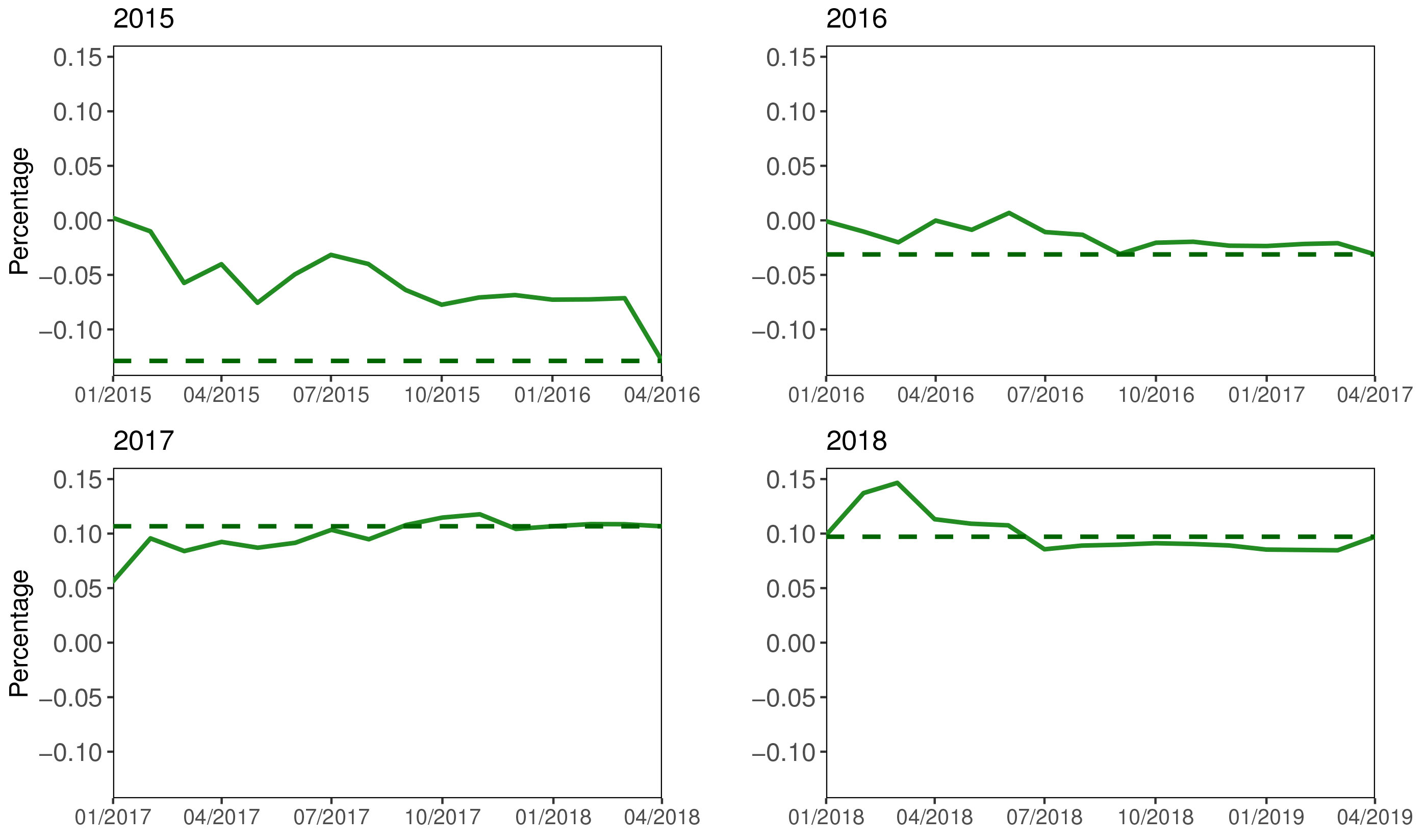

To visualize the real-time performance of the forecasts, we simulate the availability of the 26 indicators at every month since 2015.8 We then use each data vintage to estimate the model and produce a year-end forecast. The first forecast is calculated for January of the respective year, and then every month until March of the following year, the last month before the actual figure is released. This means that for the growth rate of 2015, for instance, we have monthly nowcasts from January 2015 until March 2016 and the actual figure is published in April 2016. The four panels of Fig. 2 show the results for the last four years. Given the lag structure of the model described above, a few months after the last observations, the model has no new information and the properties of the autorregresive model will dominate the dynamics. Because of this, we expect the forecasting performance to quickly deteriorate as the forecasting period is extended. Indeed, the first forecasts of each year is relatively poor. However, as new information becomes available, they rapidly improve.

4.2 Global trade in services

Services accounted for 23.4% of total international trade of goods and services in 2018.9 This share, however, has followed an increasing trend. Services are therefore an important and growing portion of international transactions. Because of their diversity and intangibility, trade in services is generally more difficult to measure than merchandise trade. However, the statistical framework for trade in services is well established and its coverage has been constantly improving as more countries implement it. Internationally-traded services can be classified according to four categories: goods-related services (3.8%), transport (17.2%), travel (23.7%) and other services (55.3%), where the numbers in parentheses refer to the share of each category in total trade in services in 2018. The group “other services” comprises a wide variety of services: construction, insurance and pension services, financial services, charges for the use of intellectual property, telecommunications and information services, other business services, personal and recreational services, and government services. Consequently, the indicators that will provide information for the nowcasting model should reflect this wide variety of economic areas.

The target variable is therefore the global value of trade in services, as reported in [30]. This is an annual time series calculated in collaboration between UNCTAD, WTO and the International Trade Center (ITC). It is compiled from data from the IMF, Eurostat, the OECD, the United Nations and other national and international sources. It is published every April, when the figures for the preceding year, based on published official data for most countries, are released. The database also includes a quarterly series for services, but its coverage is more limited and subject to large revisions, so it will not be pursued here.

Table 4
List of indicators, global exports of services

(1)	(2)	(3)	(4)	(5)	(6)	(7)
				Models
Variable	Source	Frequency	Publication lag	Initial	Core	Final
A. Sub-components of the target variable
Exports of services, United States	FRED	Monthly	2	✓	✓	✓
Exports of services, United Kingdom, series 1	TR	Monthly	2	✓	✓	✓
Exports of services, United Kingdom, series 2	OECD	Quarterly	4
Exports of services, Germany	Eurostat	Monthly	2	✓
Exports of services, France	IMF	Quarterly	4			✓
Exports of services, China	OECD	Quarterly	4
Exports of services, Netherlands	IMF	Quarterly	4			✓
Exports of services, Ireland	Eurostat	Quarterly	4
Exports of services, Japan	BOJ	Monthly	2
Exports of services, India	OECD	Quarterly	4
Exports of services, Singapore	IMF	Quarterly	4			✓
B. Structural variables
Index of export volumes, world	CPB	Monthly	3	✓	✓	✓
Suez Canal traffic statistics, net tons	SCA	Monthly	1
Panama Canal, oceangoing commercial transits	CP	Monthly	1			✓
Freight traffic of waterways, China	NBSC	Monthly	1			✓
Cargo vessel arrivals, Hong Kong	MDHK	Monthly	2
Container throughput, Hong Kong	MDHK	Monthly	3
Baltic Dry Index	TR	Monthly	1			✓
Harpex Shipping Index	TR	Monthly	1			✓
Value of exports of goods, OECD	OECD	Monthly	2	✓	✓	✓
Value of exports of goods, European Union	OECD	Monthly	2
Value of exports of goods, China	OECD	Monthly	1
Value of exports of goods, United States	OECD	Monthly	2
Value of exports of goods, Germany	OECD	Monthly	2
Tourist arrivals, world total, growth rate	UNWTO	Monthly	4	✓	✓	✓
Tourist arrivals, France	Eurostat	Monthly	6
Tourist arrivals, Spain	Eurostat	Monthly	2
Tourism receipts, United States, growth rate	UNWTO	Monthly	4
Tourist arrivals, Italy	Eurostat	Monthly	4
Tourist arrivals, Mexico	Banxico	Monthly	2
Tourist arrivals, United Kingdom	Eurostat	Monthly	4			✓
Tourist arrivals, Turkey	TSI	Quarterly	4			✓
Tourist arrivals, Germany	Eurostat	Monthly	2
Tourist arrivals, Thailand	TR	Monthly	2
Tourist arrivals, North-East Asia, growth rate	UNWTO	Monthly	4
Tourist arrivals, South-East Asia, growth rate	UNWTO	Monthly	4
Index of total manufacturing production, OECD	OECD	Monthly	3	✓	✓	✓
Index of total manufacturing production, United States	OECD	Monthly	2
Index of total manufacturing production, Japan	OECD	Monthly	2
Total inward foreign direct investment, world	OECD	Quarterly	4	✓
Total inward foreign direct investment, OECD	OECD	Quarterly	4
Total foreign direct investment, China	TR	Monthly	1
Total foreign direct investment, India	TR	Monthly	1			✓
C. Other related indicators
Index of services production, United Kingdom	ONS	Monthly	2	✓	✓	✓
Index of services production, Japan	BOJ	Monthly	2	✓
Index of services production, France	Eurostat	Monthly	5	✓
Index of services production, Brazil	IBGE	Monthly	4
Index of total retail trade value, United States	OECD	Monthly	2	✓	✓	✓
Index of total retail trade value, Japan	OECD	Monthly	3
Average unit value of exports, world	CPB	Monthly	3	✓	✓	✓
Index of free-market commodity prices	UNCTAD	Monthly	1
D. “Soft” indicators
Index of business confidence, services sector, European Union	Eurostat	Monthly	1	✓
Purchasing managers’ index, non-manufacturing, United States	TR	Monthly	1	✓	✓	✓
Purchasing managers’ index, non-manufacturing, China	TR	Monthly	1	✓	✓	✓

Table 4, continued
(1)	(2)	(3)	(4)	(5)	(6)	(7)
				Models
Variable	Source	Frequency	Publication lag	Initial	Core	Final
Purchasing managers’ index, non-manufacturing, Japan	TR	Monthly	1	✓	✓	✓
Index of consumer confidence, OECD	OECD	Monthly	1	✓
Index of consumer confidence, China	OECD	Monthly	2	✓

Sources: FRED $=$ Federal Reserve Economic Data; TR $=$ Thomson Reuters Eikon database; OECD $=$ Organisation for Economic Co-operation and Development; Eurostat $=$ Statistical Office of the European Union; IMF $=$ International Monetary Fund; BOJ $=$ Bank of Japan; CPB $=$ Netherlands Bureau of Economic Policy Analysis; SCA $=$ Suez Canal Authority; CP $=$ Canal de Panamá; NBSC $=$ National Bureau of Statistics of China; MDHK $=$ Marine Department of the Government of the Hong Kong Special Administrative Region; UNWTO $=$ United Nations World Tourism Organization; Banxico $=$ Central Bank of Mexico; TSI $=$ Turkish Statistical Institute; ONS $=$ Office for National Statistics of the United Kingdom; IBGE $=$ Brazilian Institute of Geography and Statistics; UNCTAD $=$ United Nations Conference on Trade and Development. Notes: Publication lag is the number of months between the end of the period and the time of data publication, as recorded at the moment of data collection.

The list of indicators that were considered is presented in Table 4. First, the model will include existing series of exports of services atfor the main service exporters. Although most countries only publish quarterly data as part of their balance of payments statistics, some of them also release monthly series. After this, a long list of indicators aim to capture the different types of services.

International merchandise trade and trade in services are complementary. First, because internationally traded goods need to be transported from sellers to buyers (transport is one of the types of international trade in services). Additionally, goods transported may also be subject to international insurance. Indirectly, trade in goods could also create opportunities for financial services, telecommunications, information services and other business activities. Different categories of services could then be correlated to trade volumes, trade values or both. For example, while transport will be mostly dependent of volumes, insurance costs will vary with the value of the merchandise. For this reason, we cover indicators for both volume and value of merchandise trade. For volumes, we include a monthly index of world export volumes, cargo traffic through the Panama and Suez canals, port statistics from China and Hong Kong, and the Baltic Dry and Harpex Shipping indices. For values, we consider the value of exports of goods for the largest world exporters.

Travel services are one of the main categories of international services and they can be directly measured through tourism statistics. The nowcast will test international tourism statistics for the largest destinations in the world, according to [32]. The growth rate of world tourism is also included. Since infra-annual statistics for China are not available, we add two series measuring tourist arrivals in North-East and South-East Asia.

Goods-related services refer to manufacturing services and maintenance and repair. Even if they only represent a small share of total trade in services, they could be complementary to other service categories (finance and insurance, other business services, etc.) To account for this, we incorporate industrial production indices for the OECD, United States and Japan.

Table 5

Lag order selection, global exports of services

Lag structure	Results		Results, standardized
	(1)	(2)	(3)	(4)	(5)
	$R^{2}$	MAE	$R^{2}$	MAE	Average
(8, 3)	78.2	0.0177	0.9419	0.9685	0.9552
(7, 3)	79.5	0.0179	0.9573	0.9599	0.9586
(6, 3)	79.5	0.0177	0.9578	0.9660	0.9619
(5, 3)	79.8	0.0180	0.9612	0.9545	0.9578
(4, 3)	82.2	0.0176	0.9894	0.9754	0.9824
(3, 3)	81.2	0.0178	0.9782	0.9621	0.9702
(2, 3)	81.4	0.0181	0.9799	0.9486	0.9643
(1, 3)	83.1	0.0179	1.0000	0.9581	0.9791
(8, 2)	80.2	0.0171	0.9660	1.0000	0.9830
(7, 2)	80.6	0.0177	0.9704	0.9703	0.9704
(6, 2)	80.0	0.0178	0.9634	0.9629	0.9631
(5, 2)	80.0	0.0192	0.9630	0.8912	0.9271
(4, 2)	81.2	0.0182	0.9781	0.9408	0.9595
(3, 2)	80.3	0.0186	0.9663	0.9219	0.9441
(2, 2)	39.4	0.0329	0.4746	0.5208	0.4977
(1, 2)	82.1	0.0183	0.9881	0.9387	0.9634
(8, 1)	37.4	0.0379	0.4505	0.4524	0.4515
(7, 1)	38.5	0.0373	0.4639	0.4595	0.4617
(6, 1)	38.4	0.0373	0.4627	0.4589	0.4608
(5, 1)	38.4	0.0381	0.4623	0.4493	0.4558
(4, 1)	38.4	0.0335	0.4626	0.5113	0.4869
(3, 1)	37.2	0.0337	0.4479	0.5086	0.4783
(2, 1)	38.5	0.0339	0.4639	0.5058	0.4848
(1, 1)	40.4	0.0339	0.4870	0.5051	0.4961

Figure 3.

Annual growth rates, global exports of services. Note: The line represents the estimated annual growth rate of the past 12 months with respect the 12 months before that (i.e., it is a rolling cumulative growth rate over the last 12 months). This is the main output of the nowcast model. The points represent the actual values for the growth rate. The model anchors the estimates to the actual figures, so they coincide whenever the growth rate is observed.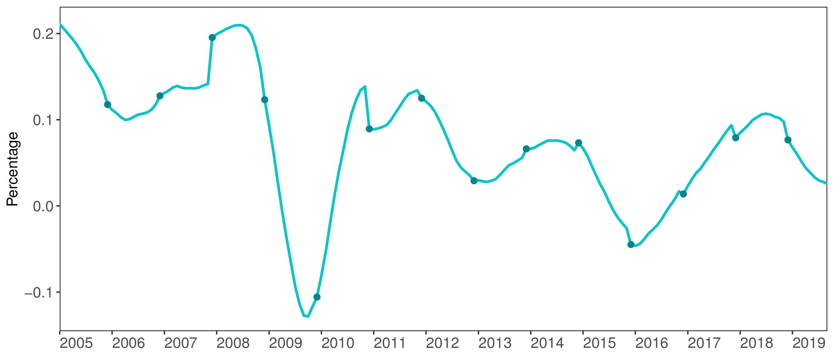

Figure 4.

Real-time growth rate forecasts, global exports of services. Note: The solid lines represent year-end growth rate forecasts produced by the nowcast model estimated with the data available at each month. The dashed lines are the actual growth rates, published in April of the following year.

Capital movements around the world also generate demand for international services, in the form of financial, insurance and other types of business activities. However, not all financial flows require the same amount of added services. Foreign direct investment (FDI) is, in principle, more service-intensive because it needs to be supported by a wider range of financial and legal services. We therefore cover this area by including FDI indicators. We consider global FDI flows, as well as inward FDI to the OECD and two of the largest emerging markets: China and India.

In addition, there are other variables that could provide relevant information to estimate trade in services. One of them is the performance of the tertiary sector in the largest exporters. However, service-specific production indices are still not common and we could only cover the United Kingdom, Japan, France and Brazil, plus the retail trade index for the United States. We also include price information (the average unit value of global exports and the commodity price index) that could directly or indirectly affect the level of traded services.

Finally, we include survey-based information that could provide timely information on the target variable. Service-specific surveys are not as common as manufacturing or overall economic activity surveys, so we will only include a business confidence index for the services sector of the European Union; non-manufacturing purchasing managers’ indices for the United States, China and Japan; and general consumer confidence indices for the OECD and China.

An initial list of 19 indicators was proposed, but this was further reduced to a core model of 12 variables after the first estimation. The initial and core models are identified in columns (5) and (6) of Table 4, respectively. The next step was the selection of the lag structure of the dynamic model, which was obtained by testing several combinations of lags terms and choosing the best performer. The results, presented in Table 5, point to a model with $m_{0}=m_{1}=8$ and $m_{2}=m_{3}=m_{4}=2$ .

A forward model selection procedure, parallel to the one described above, suggests a final model consisting of the 22 variables marked in column (7) of Table 4. The monthly estimate for the world trade in services is shown in Fig. 3. We can see that this estimate does not have such a good performance as for global merchandise trade. This is evident, for example, in the large jumps registered at the end of 2007 or 2010, caused by sudden revisions of the estimate when the final figures were published. However, the model’s performance improves considerably later in the sample. Indeed, the model is chosen so that it minimizes the forecast error over the 20% final section of the sample and the corrections in the most recent years are much smaller. In total, the model can explain 86.2% of the variability of the annual target variable.

To evaluate the forecasting accuracy of the model, we calculate a final forecast at the last data release before the final figures are published and we measure the absolute error. When we average the errors over the final 20% of the sample, to obtain a forecasting MAE of 0.0125. Figure 4 presents charts of the real-time forecasts generated by the model over the last four years. These figures show that the model correctly identifies trend changes and other dynamics of the series. For example, the model suggested a downward turn for 2015. Although it settled at a forecast of about $-$ 1%, short of the actual figure observed, it succeeded in identifying this trend reversal after five years of positive growth. For 2017, the model also correctly forecast the fast recovery in the growth rate of the target variable.

5. Conclusions

This paper presented a methodology to track the real-time evolution of global trade aggregates. This tool can be used to produce estimates of the target variables based on the most up-to-date information available. It could therefore be used to identify, in a timely manner, any changes that would require adapting economy policy in affected sectors or countries.

This model relies on dynamic factor models adapted to take into account common characteristics of this type of data: heterogeneous frequencies, missing data and ragged ends. Moreover, the solution described in Section 3 was developed in a general manner and can be adapted to a variety of target variables and underlying indicators. Additional requirements (such as infra-monthly series and data available only after known transformations) could be introduced to the model in a straightforward manner.

The results are promising. The mean absolute forecasting errors are small and the estimated factor can explain a high proportion of the variability of the target variables. The charts presented in Section 4 show that the nowcasts quickly incorporate the information provided by the underlying indicators and correctly identify changing trends and turning points. However, it must be noted that the dynamic structure of the model considers only short lags, so these models should only be used to monitor the real-time evolution of the variables and to produce short-term forecasts for periods when some of the underlying indicators are already available.

There are several ways to improve this process. First, the co-movements between the variables are constantly changing and previously tested variables may lose or gain significance when monitoring the target variables. There are also new series becoming available or receiving more widespread diffusion. The variable selection process will therefore have to be repeated frequently. Second, it could be interesting to compare the nowcasting performance when the target variable is annual or quarterly. For this exercise, we deliberately chose annual target variables since our objective is to track official data with global coverage. However, there are other series available at a quarterly frequency that, at a cost of a reduced coverage, provide more timely information on the global aggregates. Third, a potentially interesting exercise would be comparing direct nowcasts of the target series with indirect nowcasts obtained by estimating the components of the series separately (for example, the value of merchandise exports by world regions, or the value of service exports by category). Finally, as a robustness check and a potential source of improvement, we can also attempt to replicate the process with alternative methodologies, such as the EM implementation employed by [17].

Footnotes

The size of some submatrices in the measurement and transition equations may need to be adjusted in certain cases. For example, if the number of lags corresponding to the quarterly variables ( $m_{2}$ ) is greater than six, the corresponding rows and columns in all matrices need to be expanded accordingly.

Annual variables and monthly indicators expressed as year-on-year growth rates could also be considered in the model, but this would require expanding the matrices considerably. Although we will not do so here, they could be incorporated simply by including the relevant rows and columns in the matrices.

It could seem atypical to use disaggregates of the target variable as inputs to the nowcast. However, as mentioned in Section 2, this is a statistical exercise where variables are chosen because of the timely information they provide about the target variable, and not based on any causal or structural relationship. In addition, as mentioned in [], the evidence shows that adding information on disaggregates to a forecasting model of an aggregate can indeed improve forecast accuracy.

Seasonal adjustment was calculated with the R package seasonal version 1.6.1, using the default options.

Note, however, that “soft” indicators could show low significance since they normally add little information once the “hard” indicators are published. Their principal advantage is that they are available in a timely manner. They should therefore remain in the model even if their contribution seems minimal.

For the second criteria, the mean absolute error of the forecasts was also calculated at previous data vintages, without significant changes to the results. These robustness checks are available from the author on request.

We use data on world exports and not imports. At the global level, up to measurement errors and reporting issues, both are equivalent.

This is only a pseudo-real-time analysis since the actual data availability at each month is unknown. Even if we know the date of each data release, according the publication schedule of each indicator, most of the times historic data is also revised at each release and we do not have the details for each of these backward revisions.

Author calculations based on data from [].

Acknowledgments

The author would like to thank all members of the Development Statistics and Information Branch of UNCTAD for their useful discussion and suggestions during the preparation of this paper. Also, to the organizers and participants of the UNCTAD Research Seminar and the CCS-UN Technical Workshop on Nowcasting in International Organizations for the comments received.

References

Conference Board. Business Cycle Indicators Handbook. New York, NY: The Conference Board, Inc.; 2001.

OECD. OECD System of Composite Leading Indicators; 2012. Accessed on 20 July 2018. http://www.oecd.org/sdd/leading-indicators/41629509.pdf.

Baffigi

Golinelli

Parigi

. Bridge models to forecast the euro area GDP. International Journal of Forecasting. 2004; 20(3): 447–460.

Barhoumi

Benk

Cristadoro

Reijer

Jakaitiene

Jelonek

, et al. Short-term forecasting of GDP using large monthly datasets: a pseudo real-time forecast evaluation exercise. European Central Bank; 2008; 84.

Rossiter

. Nowcasting the Global Economy. Bank of Canada; 2010; 2010–12.

Stock

Watson

. Forecasting using principal components from a large number of predictors. Journal of the American Statistical Association. 2002; 97(460): 1167–1179.

Stock

Watson

. Macroeconomic forecasting using diffusion indexes. Journal of Business & Economic Statistics. 2002; 20(2): 147–162.

Forni

Hallin

Lippi

Reichlin

. The generalized dynamic factor model: one-sided estimation and forecasting. Journal of the American Statistical Association. 2005; 100(471): 830–840.

Giannone

Reichlin

Small

. Nowcasting: the real-time informational content of macroeconomic data. Journal of Monetary Economics. 2008; 55(4): 665–676.

10.

Mariano

Murasawa

. A new coincident index of business cycles based on monthly and quarterly series. Journal of Applied Econometrics. 2003; 18(4): 427–443.

11.

Camacho

Perez-Quiros

. Introducing the euro-STING: short-term indicator of euro area growth. Journal of Applied Econometrics. 2010; 25(4): 663–694.

12.

Schumacher

Breitung

. Real-time forecasting of GDP based on a large factor model with monthly and quarterly data. Deutsche Bundesbank; 2006; 33.

13.

Aruoba

Diebold

Scotti

. Real-time measurement of business conditions. Journal of Business & Economic Statistics. 2009; 27(4): 417–427.

14.

Aruoba

Diebold

. Real-time macroeconomic monitoring: real activity, inflation, and interactions. American Economic Review. 2010; 100(2): 20–24.

15.

Matheson

. New Indicators for Tracking Growth in Real Time. IMF; 2011. WP/11/43.

16.

Bańbura

Giannone

Reichlin

. Nowcasting. European Central Bank; 2010; 1275.

17.

Bańbura

Giannone

Modungo

Reichlin

. Now-Casting and the Real-Time Flow of Information. European Central Bank; 2013; 1564.

18.

Bok

Caratelli

Giannone

Sbordone

Tambalotti

. Macroeconomic nowcasting and forecasting with big data. Federal Reserve Bank of New York; 2017; 830.

19.

Ghysels

Santa-Clara

Valkanov

. Predicting volatility: getting the most out of return data sampled at different frequencies. Journal of Econometrics. 2006; 131(1–2): 59–95.

20.

Ghysels

Sinko

Valkanov

. MIDAS regressions: further results and new directions. Econometric Reviews. 2006; 26(1): 53–90.

21.

Clements

Galvão

. Macroeconomic forecasting with mixed-frequency data: forecasting output growth in the united states. Journal of Business & Economic Statistics. 2008; 26(4): 546–554.

22.

Marcellino

Schumacher

. Factor MIDAS for nowcasting and forecasting with ragged-edge data: a model comparison for german GDP. Oxford Bulletin of Economics and Statistics. 2010; 72(4): 518–550.

23.

Ferrara

Marsilli

. Nowcasting Global Economic Growth: A Factor-Augmented Mixed-Frequency Approach. Banque de France; 2014; 515.

24.

Guichard

Rusticelli

. A Dynamic Factor Model for World Trade Growth. OECD; 2011; 874.

25.

Golinelli

Parigi

. Tracking world trade and GDP in real time. International Journal of Forecasting. 2014; 30(4): 847–862.

26.

Barhoumi

Ferrara

. A World Trade Leading Index (WTLI). IMF; 2015. WP/15/20.

27.

Burgert

Dées

. Forecasting World Trade: Direct versus “Bottom-Up” Approaches. European Central Bank; 2008; 882.

28.

Hendry

Hubrich

. Forecasting Economic Aggregates by Disaggregates. European Central Bank; 2006; 589.

29.

Unites States Census Bureau. X-13 ARIMA-SEATS Seasonal Adjustment Program; 2017. Accessed on 20 July 2018. https://www.census.gov/srd/www/x13as.

30.

UNCTAD. UNCTADstat. Accessed on 31 October 2019. https://unctadstat.unctad.org.

31.

United Nations Statistics Division. National Accounts – Analysis of Main Aggregates (AMA). Accessed on 31 October 2019. https://unstats.un.org/unsd/snaama.

32.

World Tourism Organization. UNWTO Tourism Highlights: 2018 Edition. Madrid, Spain: UNWTO; 2018.

Nowcasting global trade in goods and services

Abstract

Keywords

1. Introduction

2. Nowcasting global trade

3. The nowcasting model

3.1 Mixed frequencies

3.1.1 Annual variables

3.3.1 Annual target variable

4. Empirical analysis

4.1 Global trade in goods

Table 1 List of indicators, global exports of goods

Table 4 List of indicators, global exports of services

Footnotes

Acknowledgments

References

Table 1
List of indicators, global exports of goods

Table 4
List of indicators, global exports of services