
Abstract
Over the last several years and within the framework of the Sustainable Development Goals, there has been a need to improve the measurement and understanding of local geographic patterns to support more decentralized decision-making and more efficient program implementation. This requires more disaggregated data that are not currently available in a nationally representative household survey.
This study explores the potential of model-based geostatistics methodology to model DHS survey indicators. We implement a stacked ensemble modeling approach that combines multiple model algorithmic methods to increase predictive validity relative to a single modeling. The approach captures potentially complex interactions and non-linear effects among the geospatial covariates. Three submodels are fitted to six DHS indicator survey data using the geospatial covariates as exploratory predictors. The model prediction surfaces generated from the submodels are used as covariates in the final Bayesian geostatistical model, which is implemented through a stochastic partial differential equation approach in the integrated nested Laplace approximations.
The proposed approach can help to inform the allocation of resources and program implementation in areas that need more attention. Countries can use this approach to model other DHS survey indicators at much smaller spatial scales.
Background and objectives
Background
The Demographic and Health Surveys (DHS) Program has been a leader in collecting and providing cluster-randomized survey data on various development and health indicators. In addition to the standard open-source data files in which household and individual survey results can be tabulated by first-order subnational units (states/provinces or regions) andurban/rural strata, more surveys are now providing georeferenced data for individual clusters. The availability of the Global Positioning System (GPS) coordinates for DHS, the Malaria Indicator Survey (MIS), and the AIDS Indicator Survey (AIS) clusters provides highly local scale information that can be linked with survey outputs for quantifying demographic and health status heterogeneities and inequities.
During the last several years and within the framework of the Sustainable Development Goals (SDGs), there has been an expressed need to improve the measurement and understanding of local geographic patterns in order to support more decentralized decision-making and more efficient program implementation [1]. This requires additional disaggregated data that are not currently available in a nationally representative household survey.
Analyses of the DHS survey indicators are conducted primarily at the national level, but also at the first subnational administrative level (Admin 1). Since estimates produced at the national level are more useful for making comparisons between nations and aggregating across large world regions, their natural audience includes international policymakers and donors [2]. However, the Admin 1 analysis does not provide comprehensive estimates at lower levels, such as the second subnational administrative level (Admin 2), where health programs are designed and implemented.
To better address the need for fine spatial and lower administrative level estimates, there are three possible options: (i) Scaling-up the nationally representative survey data collection process by increasing the sample size, survey costs, and survey time to create a representative sample at the desired administrative level. (ii) Using data derived from routine health management information systems (HMIS) from health facilities, communities, census, or other household surveys, such as data that can determine the vaccination coverage in a district. (iii) Creating spatially interpolated maps that use modeling techniques to predict values at non-surveyed locations.
Increasing DHS survey sample size to enable increased geographic disaggregation is both time consuming and expensive. Thus, the first option may not be feasible in an increasingly resource-constrained environment. With the second option, HMIS data quality is not always reliable, and the data are not easily accessed. The third option, which uses spatial modeling techniques that leverage existing survey data, spatial relationships between survey clusters, and relationships with geospatial covariates, has become increasingly popular in mapping key development indicators at high spatial resolution [3, 4].
The Bayesian spatial approach is increasingly recognized as an excellent geostatistical analysis method for addressing uncertainty in the model estimates and for being flexible and capable of handling missing data [5]. This approach has been widely used to predict and map various indicators such as those described in SAR 11 [6], poverty [7], and malaria [8, 9, 10, 11, 12, 13, 14, 15]. In these studies, environmental data layers that are thought to influence the indicators are used to explain some of the variations in prevalence across different areas. This can aid our understanding of the relationships between the indicator and the influence of climatic/environmental and socioeconomic factors [16].
The Markov Chain Monte Carlo (MCMC) algorithms have been the most common method for making Bayesian statistical inferences with generalized linear geostatistical models (GLGM) [17]. The MCMC has been developed for model estimation, but can be computationally expensive, especially with big data. There has been a recent increase in the application of integrated nested Laplace approximation (INLA) methodology and software (
Objectives
In this study, we explore the potential of model-based geostatistics (MBG) methodology (described in the methods section) to model DHS survey indicators. More specifically, we use the stacking and ensemble model approaches to predict the indicators at a high-resolution gridded pixel level, and produce estimates at the Admin 2 level. The INLA methodology is used to create a model for predicting the indicators based on the different geospatial covariates and spatially correlated random effects, and to produce prediction maps. The report will develop R code structure and workflow for routine interpolation of survey data at the second subnational administrative level (Admin 2).
Methods
A modeling framework for generating standardized modeled surfaces using DHS survey data has been described in SAR 11 [6] and SAR 14 [19]. In this analysis, we employed a new geospatial modeling approach similar to that used in mapping of child growth failure [20], education attainment [21], vaccine coverage [22], HIV [23], exclusive breastfeeding [24], and childhood diarrheal diseases [25]. We adopted this method because it has been shown to improve the prediction accuracy based on the stacked generalization that allows for multiple, non-linear algorithmic mean functions to be embedded within a Gaussian process framework [26]. We detail this approach in the next sections.
DHS indicators
The DHS indicators included in the analysis were extracted from two national DHS surveys, the Kenya 2014 DHS and Ethiopia 2016 DHS. We considered data only from those surveys that had described the total number of individuals examined, the proportion of positive cases, and the coordinates of their geographical locations. From these surveys, we obtained 1,583 and 620 clusters for Kenya and Ethiopia, respectively. Table 1 describes the indicators we modeled.
Description of DHS indicators
Description of DHS indicators
Geospatial covariates used to develop the models
To model the DHS indicators, we assembled environmental and socioeconomic geospatial covariate data layers, which were obtained from publicly available remote sensing sources. These data included access (travel time to nearest settlement), aridity, diurnal temperature range, precipitation, potential evapo-transpiration (PET), daily maximum temperature, elevation, enhanced vegetation index (EVI), daytime land surface temperature, diurnal difference in land surface temperature, night land surface temperature (LST), and population categories (children under age 5, women age 15 to 49, and total population). Further description of each covariate can be obtained from the DHS Geospatial Covariate Report [27].
The geospatial covariates were selected for their potential to predict DHS indicators, and they have previously been shown to correlate with the development of indicators in different settings [6, 28]. Table 2 describes the spatial and temporal resolution of each geospatial covariate and the sources.
Geospatial covariates processing
The geospatial covariate data layers used in this analysis were acquired from a myriad of data sources, and therefore have different spatial references, projections, extents, and dimensions. For example, gridded population data and elevation had a 1
Geospatial modeling flowchart.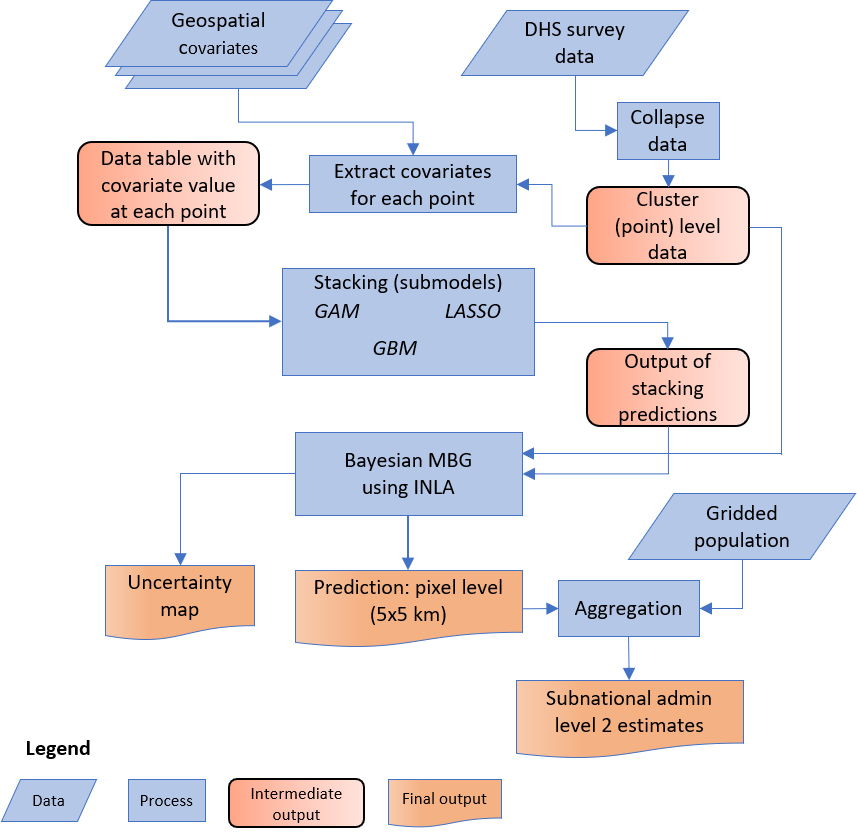
Overview of the modeling approach
Figure 1 depicts the geospatial modeling framework used for modeling DHS indicators and the underlying covariates and producing the gridded pixel and subnational level estimates. The approach involved the following steps: Step 1 – We summarized the individual-level DHS survey data to the finest spatial resolution (latitude and longitude) that represented the location of the survey cluster. Step 2 – The processed geospatial covariates (from the previous section) and the cluster (point) level data were imported into the R environment for statistical computing [29]. We then applied the ‘raster’ package to extract the corresponding covariate pixel values at each survey cluster point. Step 3 – The point level data (from Step 2) and their associated geospatial covariates were used in the stacked (submodels) generalization ensemble model. The prediction surfaces generated from the stacked ensemble models were then used as covariates in the final geospatial (MBG) model. The outputs of the final model are pixel-level mean estimates at the 5
Covariate ensemble modeling using stacked generalization
Stacking (also called stacked generalization/regression) is an ensemble modeling approach that combines multiple model algorithmic methods to increase predictive validity relative to a single modeling approach. We employed this approach to capture the potential complex interactions and non-linear effects among the geospatial covariates. The ensemble approach has been shown to improve the predictive accuracy of the geostatistical models, as compared to prediction from any single method [26]. Numerous recent studies have implemented the stacking approach to derive continuous estimated surfaces of indicators of interest from DHS household surveys. These include mapping of HIV prevalence [23], vaccine coverage [22], exclusive breastfeeding [24], child growth failure [20], education attainment [21], and childhood diarrheal diseases [25].
In our analysis, we fitted three submodels to each set of the selected DHS indicator survey data using the geospatial covariates (described in Table 2) as exploratory predictors. These include (i) GAM: generalized additive model [30], (ii) LASSO: least absolute shrinkage and selection operator regression [31] and (iii) GBM: gradient-boosted trees [32]. The submodels were implemented in R statistical for the computing environment using packages ‘caret’, ‘mgcv’, ‘xgboost’, and ‘glmnet’. We selected these model algorithms because they have demonstrated high predictive accuracy in previous studies [33, 34, 35, 36, 37, 38, 39, 40, 41, 42, 43].
To make better predictions and avoid overfitting, each submodel was fit using five-fold cross-validation, which generated the out-of-sample predictions that were included as exploratory geospatial covariates when fitting the geostatistical model. In addition, each submodel was fit with a full dataset, which produced the in-sample predictions that were then used as covariates when generating predictions from the full geostatistical model. A logit transformation of the predictions was used to place the out-of-sample and in-sample predictions on the same scale as the linear predictor in the geostatistical model. This process has been described in detail [23, 26].
Model specification and development
As described in the previous section, the ensemble modeling approach allows for non-linear relationships and interactions between the geospatial covariates to better predict the DHS indicators. Since the approach does not explicitly account for spatial patterns in the data, we used the Bayesian geostatistical modeling framework in our analysis to account for the spatial dependence.
For each indicator of interest, we modeled
Where:
The spatial error term
The spatial covariance
Where
The Bayesian geostatistical model analysis was implemented through a stochastic partial differential equations (SPDE) approach in the recently developed INLA algorithm as applied in the R-INLA package [18]. This algorithm provides an effective estimation and spatial prediction strategy for spatial data by specifying a spatial data process as well as a spatial covariance function depending on locations and time points at which infection and covariate data are collected [18]. The INLA approach offers an advantage of providing accurate and fast results as compared to the MCMC algorithms, which are known to have problems of convergence and dense covariate matrices that increase the computational time. Thus, for large datasets, spatial and spatiotemporal estimation could lead to several days of computing time [18, 47, 48].
Predicted surfaces for stunting in Kenya generated from the three submodels (GAM, GBM, and LASSO).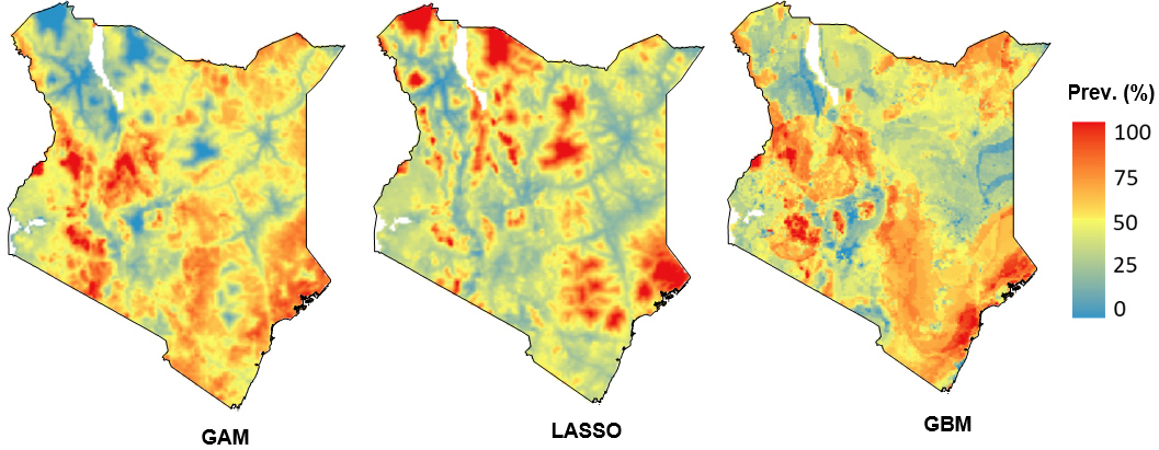
Predicted surfaces for stunting in Ethiopia generated from the three submodels (GAM, GBM, and LASSO).
Pixel level prediction of prevalence of the indicators modeled by using the Kenya DHS 2014: (a) Stunting, (b) Wasting, (c) Vaccine DPT3, (d) ANC visits, and (e) Water sources.
Pixel level prediction of prevalence of the indicators modeled by using the Ethiopia DHS 2016: (a) Stunting, (b) Wasting, (c) Vaccine DPT3, (d) ANC visits, (e) Water sources, and (f) Women’s anemia.
Second subnational administrative level estimates for Kenya DHS 2014: (a) Stunting, (b) Wasting, (c) Vaccine DPT3, (d) ANC visits, and (e) Water sources.
The prediction surfaces generated from the ensemble submodels were used as input covariates in the geostatistical models implemented in INLA. The final estimates for each indicator were generated by taking
Model estimates at admin level 2
In addition to the 5
Model validation
For each of the indicator model outputs, we implemented a validation procedure and calculated a set of performance statistics. This involved using an out-of-sample cross-validation with a five-fold hold-out procedure and a comparison of the predicted values at the locations of the hold-out data with their observed values. This procedure was repeated five times without replacement so that every data point was omitted one time across the five validation runs. Standard validation statistics were then computed as measures of the predictive accuracy of the modeled estimates. This included mean absolute error (MAE), mean error (ME) or bias; root-mean-squared-error (RMSE, which summarizes the total variance); and 50%, 80%, and 95% coverage of our predictive intervals aggregated to the spatial holdout level. Each predictive metric was calculated by first simulating predictive draws using a binomial distribution. The predictive metric of interest was then calculated as a sample-size-weighted mean over the second administrative levels [22]. To complement the out-of-sample predictive validity metrics, we also calculated in-sample predictive validity metrics that used the same process but matched each data point to predictions from a model fitted with all data.
Results
Stacking results
Here we present results obtained from the individual submodels according to the environmental and socioeconomic predictor variables in our model. The submodels revealed that the prediction of the DHS indicators varies spatially in the different areas in the country. Figures 2 and 3 represent prediction areas with high and low prevalence of stunting for the Kenya DHS 2014 and Ethiopia DHS 2016 surveys that we generated from the three submodels.
Predictive metrics for each indicator aggregated at admin 2 (Kenya)
Predictive metrics for each indicator aggregated at admin 2 (Kenya)
Second subnational administrative level estimates for Ethiopia DHS 2016: (a) Stunting, (b) Wasting, (c) Vaccine DPT3, (d) ANC visits, (e) Water sources, and (f) Women’s anemia.
Prediction prevalence maps for each indicator were created using the full geospatial Bayesian model. Figures 4 and 5 show the pixel level prediction surface maps for Kenya and Ethiopia, respectively. Areas with high and low estimated prevalence of each indicator can be seen clearly across all maps.
Admin level 2 estimates
Figures 6 and 7 show the second subnational administrative level estimates that highlight areas with high and low prevalence of each indicator we modeled.
Predictive metrics for each indicator aggregated at admin 2 (Ethiopia)
Predictive metrics for each indicator aggregated at admin 2 (Ethiopia)
Comparison of predictions for each indicator, aggregated to the second subnational administrative level with 95% uncertainty intervals, plotted against data observations from the same area aggregated to the second subnational administrative level for Kenya.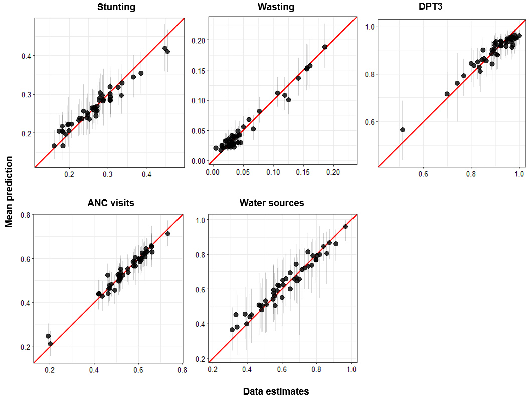
Comparison of predictions for each indicator, aggregated to the second subnational administrative level with 95% uncertainty intervals, plotted against data observations from the same area aggregated to the second subnational administrative level for Ethiopia.
Model validation was performed by calculating bias (mean error); mean absolute error (MAE); variance (RMSE); 50%, 80%, and 95% data coverage within prediction intervals; and the correlation between observed data and predictions.
Results from the validation indicated the best performance for each indicator, where correlation increased with decreased MAE and RMSE values. The coverage values for some indicators (vaccine) were too high, which was most likely a result of high uncertainties that arise from the small sample at the cluster locations (Tables 3 and 4).
Comparison of model estimates versus DHS estimates
Figures 8 and 9 show the comparison estimates for each indicator produced by the models in our analysis and the equivalent estimates from the observed DHS survey data. The results indicate a high correlation between MBG and DHS estimates for most indicators.
Discussion and conclusion
In recent years, there has been a need for district (Admin 2) estimates currently not available in a DHS survey. In an increasingly resource-constrained environment, high resolution maps of key health indicators and development derived from cluster point data through spatial interpolation methods offer an attractive solution.
In this analysis, we developed a methodological framework for estimating DHS indicators at the Admin 2 level. We took advantage of the advancement in geospatial technologies, availability of free and open-source spatial data, and geospatial software tools relevant for spatial modeling. This framework used an ensemble modeling approach that combines multiple model algorithmic methods to increase predictive validity relative to a single modeling approach. We employed this approach to capture potential complex interactions and non-linear effects among the geospatial covariates. We fitted three submodels (GAM, LASSO, and GBM) to each of the selected DHS survey indicator data using the geospatial covariates as exploratory predictors. The submodels were selected because they were available in standalone packages that required minimal data preparation after the predictor variables had been produced; they are particularly useful in cases where presence-only data are available [35, 49, 50] and have been successfully used in previous analyses that have implemented the stacking approach to derive continuous estimated surfaces of indicators of interest from the DHS household surveys. These include mapping of malaria [26], HIV prevalence [23], vaccine coverage [22], exclusive breastfeeding [24], child growth failure [20], education attainment [21], and childhood diarrheal diseases [25].
We found variability in the individual model prediction outputs. For example, the LASSO model output indicated a low prediction of stunting in the northeast areas of Kenya (Fig. 2) as compared to the other algorithms. This could be explained by the prediction uncertainties in the individual submodels [35, 49]. Using different models and combining them in an ensemble model could improve these uncertainties [51, 52, 53]. Our findings demonstrated that the predictions from the stacking ensemble model approach were more accurate than those from the individual model algorithms. The results suggest that use of an ensemble model approach is more adequate than predictions from any single modeling methods. These findings are consistent with other studies [26, 52], which showed the ensemble model approach to be the best. By developing the methodological framework within the R statistical computing environment, we have created a tool that can be used to model other health indicators.
The results from the Admin 2 level, generated from the full geostatistical model, show that the estimated prevalence of each indicator varied across the different areas in the country.
Although we have estimated the prevalence for each indicator at the pixel-level and the Admin 2 level, our study has some limitations. Our analysis used a suite of standard geospatial covariates that included those that are not directly related to the indicators we modeled. To improve predictions, further studies should restrict the model input data to those covariates associated with the indicators of interest. Due to computational limitations, we did not quantify uncertainty in the covariates and submodel estimates. Thus, further analysis should develop methods that are capable of propagating uncertainty in both the covariates and submodel estimates [23, 54].
We generated maps showing estimates of high-risk areas for each indicator we modeled. Our approach in this analysis can help inform the allocation of resources and program implementation in areas that need more attention. Interventions and programs that can be implemented and directed at much smaller spatial scales using the MBG estimates such as the one described in our analysis could enable better programmatic decisions.
Footnotes
Acknowledgments
The authors would like to thank the external reviewers for the careful review and thoughtful comments.
This work was supported by the United States Agency for International Development (US) (USAID) through The DHS Program (#720-OAA-18C-00083). Views expressed are those of the authors and do not necessarily reflect the views of the USAID or the United States government.