Understanding financial distress by using Markov random fields on linked administrative data

Abstract

Household financial distress is a complicated problem. Several social problems have been identified as potential risk factors. Conversely, financial distress has also been identified as a risk factor for some of those social problems. Graphical models can be used to better understand the co-dependencies between these problems. In this approach, problem variables are network nodes and the relations between them are represented by weighted edges. Linked administrative data on social service usage by $6,848$ households from neighbourhoods with a high proportion of social housing were used to estimate a pairwise Markov random field with binary variables. The main challenges in graph estimation from data are ( $a$ ) determining which nodes are directly connected by edges and ( $b$ ) assigning weights to those edges. The eLasso method used in psychological networks addresses both these challenges. In the resulting graph financial distress occupies a central position that connects to both youth related problems as well as adult social problems. The graph approach contributes to a better theoretical understanding of financial distress and it offers valuable insights to social policy makers.

Keywords

Markov random fields financial distress social policy linked administrative data

1. Introduction

Household poverty and debts are complex problems. For both types of financial distress, researchers have identified numerous risk and protective factors, which range from the individual level to various layers of the broader social context [1, 2, 3, 4, 5, 6, 7, 8, 9, 10, 11, 12, 13, 14]. This context includes societal, political and macro-economical influences [15, 16, 17]. Yet, according to some authors, this research has not led to a comprehensive theoretical understanding of the causes of financial distress [18, 19]. One possible explanation these authors offer for this absence, is that a comprehensive framework requires the combined effort of several scientific disciplines (e.g. psychology, sociology, economics). This is certainly indicative of one aspect of the complexity surrounding financial distress. Another aspect of this complexity is the difficulty in establishing the direction of the relationship between financial distress and certain suspected risk factors [20], because some of the known risk factors are also among the many potential consequences of financial distress. These include the impact of financial distress on physical health [21, 22, 11, 23], mental health [24, 25, 26, 27, 28], workplace performance [29], and cognitive functioning [30, 31, 32, 33, 34]. For instance, mental health problems may be found to increase the risk of financial distress, but the connection could also be the other way around (i.e. financial distress increases the risk of mental health problems), or there could be a reciprocal relationship between them [35, 36, 37].

Because of such reciprocal effects, it may not be helpful to regard financial distress only as an outcome that is to be explained by a set of known risk and protective factors. Rather, in order to better understand financial distress, we argue that it should be considered as one element within a broader network of interrelated variables. Thus, to better understand financial distress, we should seek to understand this broader network. Psychological networks are used for similar reasons [38, 39].

The structure of this network of variables can then reveal (1) which nodes (problem variables) occupy a central position, so that any change in these nodes is likely to reverberate through the entire network, and (2) which edges (relationships) play a key part in conducting such cascades, so that reducing these dependencies is likely to reduce the overall sensitivity of the network to the impact of adverse changes [39, 40].

Thus, the network-of-variables approach can potentially provide both theoretical insight to social scientists as well as valuable directions for intervention targets to policy makers and social care professionals. In this paper, we propose to describe financial distress within a broader network of variables by analysing a dataset of municipal household register data with statistical graphical models. We will explore how a network structure can be derived from data on financial distress and other problems; and whether the resulting network can be meaningfully interpreted with respect to social policy.

In this context, a graphical model describes a set of variables (nodes) and their undirected conditional relationships (edges). To illustrate this idea, Fig. 1 gives a reduced version of our larger result – discussed in Section 4 – as an example. This small graph shows the relations between household debt, financial support (FinSup), general youth care (GCyth), school absenteeism (Abs) and NEET (Not in Education, Employment or Training). The width of the edges signifies the relative strength of the undirected conditional relationships [41, 42, 43, 44].

The graph shows that educational problems in households (absenteeism, NEET) are not directly connected to debt, but that there are indirect connections through general youth care and financial support. Although this limited graph is given here only for illustration, the potentially interesting role of municipal youth care and its relations is apparent, since educational problems appear to be linked to financial distress mainly through general youth care. This suggests targets for study and intervention. We will further explore such relations in what follows.

Figure 1.

Graph of the variables (a) financial distress, financial support (FinSUp) and debt; educational problems, absenteeism (Abs) and Not in employment, education or training (NEET); and receiving general youth care (GCyth).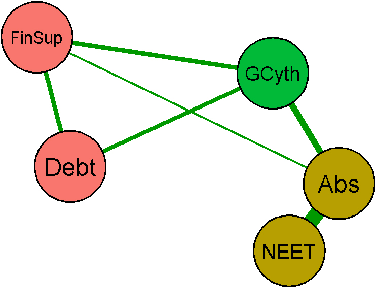

Section 2 describes the specific graphical model that is to be estimated (a pairwise Markov random field with binary variables), the eLasso method of neighbourhood selection to estimate the model, as well as a number of ways to evaluate the resulting graph. The data set is introduced in Section 3 and the graph that was estimated from these data is presented and discussed in Section 4. Finally, Section 5 provides a discussion and conclusion.

2. Methods

2.1 Model definition

The core principle of graphical modelling is the representation of variables as nodes and relationships between variables as edges in a graph. Modelling a variable of interest, such as financial distress, within a larger “network”, or graph, of variables is an idea with a long history, encompassing at least two traditions. First, that of directed models, due originally to Wright in 1921 [45], which developed into modern-day “structural equation models” (SEM [46]; and their modern variations [47]), and “structural causal models” [48]. The advantage of these approaches is that, if the directions of the “arrows” in the model are known in advance, estimation yields causal quantities of interest [48]. Their disadvantage is that they require deep a priori knowledge of the underlying causal process as an identification strategy [49].

A second tradition, perhaps less employed within the social sciences, is that of undirected graphical models, due originally to Gibbs in 1902 [50] and Ising in 1925 [51], and applied as “Markov random fields” in a variety of fields including statistical physics, protein function prediction, image analysis, and spatial statistics [42, 52]. These models have the disadvantage that their parameters are not interpretable as causal parameters of interest. Their advantage, however, is that causal “flow” between variables can still be represented without a priori determinations of the directions of causality between the variables [42]. For this reason, they have enjoyed a recent revival within psychological studies as a flexible way of studying constellations of variables on which less information regarding their precise causal interactions is available [53, 54, 55, 56, 57, 58, 59, 60, 61, 62, 63]. For the same reasons, we adopt Markov random fields as a convenient framework to study financial distress and its interactions with other variables.

Markov random fields may be parametrised in various ways, depending on the type of variables (discrete or continuous) and whether higher-order interactions are thought to be important. In this work, we will concentrate on a model for binary (dichotomous) variables, in which only pairwise interactions are modeled – that is, a “binary pairwise Markov random field”. Note that this model can also be seen as a loglinear model [64, 65] for the cross-classification of all variables with interactions up to order two; we prefer to use the term Markov random field, to emphasise that the model is part of a family of undirected graphical models that can also be applied to data sets with continuous variables [66]. The nodes in the model are random variables that are either in state $0$ (“off”) or $1$ (“on”). Nodes that are directly connected by an edge are called neighbours. Not all nodes are necessarily directly connected by edges. The probability for a node to be $0$ or $1$ depends on the states of the neighbouring nodes. The strength of this interaction between neighbours is expressed as an edge weight. Additionally, a parameter is assigned to each individual node to express the “natural” tendency of that node towards $0$ or $1$ independent of its neighbours.

Legend 1: Notation
$X_{j}$ : Node $j$ , a random variable.
$p$ : Number of nodes in the graph.
$\theta=(\alpha_{j},\beta_{j,k})$ : vector of model parameters.
$\theta_{j\|-j}$ : Parameter vector of logistic regression model (Eq. (2)) with node $X_{j}$ as outcome variable. Note that the outcome of the model is conditional on the value of all nodes except node $X_{j}$ , hence “ $j\|-j$ ”.
$V=\{X_{1},X_{2},\ldots,X_{p}\}$ : set of binary nodes.
$V_{c}$ is configuration $c$ out $C=2^{p}$ possible node configurations of $V$ .
$x^{(c)}_{j}$ : The value that node $X_{j}$ takes under configuration $V_{c}$ .
$A=\{\alpha_{1},\alpha_{2},...,\alpha_{p}\}$ : set of node parameters.
$E$ : adjacency matrix of weighted edges with non-zero elements $\{\beta_{1,2},...\beta_{j,k},\beta_{p-1,p}\}$
$G(A,V,E)$ : the model graph.
$\mathcal{D}=(\mathbf{d}_{1},\ldots,\mathbf{d}_{n})$ : A dataset of $n$ observations, where $\mathbf{d}_{i}$ is the $i$ th observation of $V_{i}$ = $(\mathbf{x}_{1(i)},\ldots,\mathbf{x}_{p(i)})$

The node tendencies $\alpha_{j}$ and edge weights $\beta_{j,k}$ are the model parameters (see Legend 1). Let $G(A,V,E)$ be a graph with $p$ nodes, defined by a set of node parameters $A=\{\alpha_{1},\alpha_{2},\ldots,\alpha_{p}\}$ , a set of binary nodes $V=\{X_{1},X_{2},\ldots,X_{p}\}$ and an adjacency matrix $E$ with edge weights $\beta_{j,k}$ :

$\displaystyle E=\left[\begin{array}[]{ccccc}0&\beta_{1,2}&\beta_{1,3}&\ldots&% \beta_{1,p}\\ &0&\beta_{2,3}&\ldots&\beta_{2,p}\\ &&0&\beta_{j,k}&\ldots\\ \omit\span\omit\text{Sym.}&&0&\beta_{p-1,p}\\ &&&&0\\ \end{array}\right].$

Note that there are no self-interacting nodes in this model, which means that the edge weights on the diagonal of the matrix are all 0. Edges have no directions, making $E$ symmetric. If nodes are not neighbours (i.e. not directly connected), then the corresponding edge has weight $0$ .

Let configuration $V_{c}$ denote a specific combination of states for all nodes in the node set $V$ . With $p$ binary nodes, the total number of possible configurations is $C=2^{p}$ . While any of these configurations may occur, some configurations have a higher probability of occurring than others, as determined by the model parameters. This probability is modelled using an exponential-family probability function. The joint probability $\text{Pr}(V_{c})$ for a graph with $p$ nodes to have a particular configuration of node values $V_{c}$ out of all $C=2^{p}$ possible configurations is given by

$\displaystyle\text{Pr}(V_{c})=\text{Pr}(X_{1}=x^{(c)}_{1},\ldots,X_{p}=x^{(c)}% _{p})=$ (1) $\displaystyle\frac{\exp{\left(\sum_{j=1}^{p}\alpha x^{(c)}_{j}+\sum_{j\neq k}% \beta_{j,k}x^{(c)}_{j}x^{(c)}_{k}\right)}}{\sum_{c^{\prime}=1}^{2^{p}}\exp{% \left(\sum_{l=1}^{p}\alpha x^{(c^{\prime})}_{l}+\sum_{l\neq m}\beta_{l,m}x^{(c% ^{\prime})}_{l}x^{(c^{\prime})}_{m}\right)}}$

Since the edge weights $\beta_{j,k}$ are non-zero precisely when $X_{j}$ and $X_{k}$ are neighbours in the graph, only direct neighbours contribute to the odds of a specific configuration (known as the local Markov property [67]), thus creating a link between the graphical representation and the joint probability model in Eq. (1). The local Markov property is sometimes helpful when interpreting model results. For example, it implies that any “causal flow” between groups of variables through the graph can be throttled by intervening on variables that represent a bottleneck for this flow. In Fig. 1, for instance, intervening on the variable “GCyth” would be predicted to prevent a knock-on effect of educational problems on financial distress and vice-versa.

The denominator – also known as the “partition function” – in Eq. (1) contains a summation over all $2^{p}$ possible configurations. With a large number of nodes, partition function computation can become computationally infeasible [68, 69]. MRFs, however, have the convenient and well-known property that the intractable parameter estimation problem can be reduced (by approximation) to a series of (logistic) regression problems, a fact that greatly facilitates estimation [70]. This approach utilises the local Markov property of MRFs. Let $\mathbf{x}_{-j}$ denote the values of all nodes except $\mathbf{x}_{j}$ . Given $\mathbf{x}_{-j}$ , the conditional probability for node $X_{j}$ to equal 1 follows from the partial derivative of the multivariate numerator in Eq. (1) [71, 72]:

$\displaystyle\text{Pr}\left(X_{j}=1|\mathbf{x}_{-j}\right)=\frac{\exp\left(% \alpha_{j}+\displaystyle{\sum_{k}}\beta_{j,k}x_{k}\right)}{1+\exp\left(\alpha_% {j}+\displaystyle{\sum_{k}}\beta_{j,k}x_{k}\right)}$ $\displaystyle=\left(1+e^{-(\alpha_{j}+\sum_{k}\beta_{j,k}x_{k})}\right)^{-1}$ (2)

The final part of Eq. (2) is of course a familiar expression. It shows that for every node, the conditional probability (i.e. conditional on all other nodes) to turn “on” is simply a logistic probability (“sigmoid”) function, in which the independent variables are the direct neighbours of the node. A difference between the MRF and a series of logistic regression models is that in the MRF the coefficients $\beta_{j,k}$ are shared between nodes. In other words, in the MRF a coefficient $\beta_{j,k}$ determines both the effect of node $X_{j}$ on node $X_{k}$ , as well as the effect of node $X_{k}$ on node $X_{j}$ .

2.2 Model estimation, including structure estimation

Given a fully observed dataset $\mathcal{D}=(\mathbf{d}_{1},\ldots,\mathbf{d}_{n})$ of $n$ i.i.d. observations, the likelihood of the data is given by the standard i.i.d. joint log-likelihood,

$\displaystyle\ell(\theta)=\log\text{Pr}(\mathcal{D}|\theta)=\sum_{i=1}^{n}\log% \text{Pr}(\mathbf{d}_{i}),$ (3)

where $\text{Pr}(\mathbf{d}_{i})$ is the joint probability, given in Eq. (1), of the configuration $V_{c}$ that corresponds to $\mathbf{d}_{i}$ . There are then two challenges in estimating this model. First, the joint likelihood involves the often computationally infeasible partition function. Second, the structure of the graph is unknown, so that the pattern of zeroes in the adjacency matrix $E$ must be estimated.

Both challenges can be addressed by leveraging the logistic form of the model shown in Eq. (2). Instead of directly optimizing Eq. (3) and computing $2^{p}$ configuration joint probabilities in each iteration, $p$ logistic regression likelihoods are combined. The choice of a specific method of combining these regression models, which share some of their parameters, then addresses the first challenge. The second challenge can be addressed by noting that the selection of edges in this set of logistic models is equivalent to the problem of model specification search in logistic regression, for which a number of solutions exist. Although in complete generality the model selection problem is in itself NP-hard, a convenient approximate solution is to apply L1 (“LASSO”) penalization [73] to each regression problem separately [74, 75]. Since the LASSO has solutions that constrain some of the coefficients (edges) to equal zero, this procedure results in an estimation of the pattern of zeroes in the adjacency matrix.

Here we follow the proposals of Ravikumar et al. [74] and van Borkulo et al. [53] for the estimation of binary pairwise MRFs:

For each node $X_{j}$ , an L1-penalized (“LASSO”) logistic regression model is fitted according to Eq. (2). That is, the sample estimate $\hat{\theta}_{j|-j}=\max_{\theta}\ell_{\text{LR}}(\theta_{j|-j})$ is obtained by maximizing the objective

$\displaystyle\ell_{\text{LR}}(\theta_{j|-j})\!=\!\sum_{i=1}^{n}\log\text{Pr}(X% _{j}=\mathbf{x}_{j(i)}|\mathbf{x}_{-j(i)})$ $\displaystyle\quad+\lambda\sum_{j,k}|\beta_{j,k}|,$ (4)

where $\theta_{j|-j}$ is the model for node $X_{j}$ conditional on the state of all other nodes (i.e. “ $-j$ ”), $x_{j(i)}$ is the $i$ th observation of the outcome node, $\text{Pr}(X_{j}=\mathbf{x}_{j(i)}|\mathbf{x}_{-j(i)})$ is the conditional probability given in Eq. (2) and $\lambda$ is a penalization parameter such that higher values will generate a sparser graph.

Using the method described by Friedman et al. [76], for each of the $p$ models, the logistic likelihood $\ell_{\text{LR}}(\theta_{j|-j})$ is computed for a set of $100$ possible values of the penalization parameter $\lambda$ ; the extended Bayesian information criterion (“eBIC”) score [77] is then determined for each of the $100$ potential models:

$\displaystyle\text{eBIC}_{j}=-2\ell_{\text{LR}}(\hat{\theta}_{j|-j})∼{}+∼{}J% \cdot\log(n)∼{}+2\gamma J\cdot\log(p∼{}-∼{}1).$ (5)

Here, the number of neighbours selected is $J$ . The regular BIC is extended by the addition of $2\gamma J\cdot\log(p∼{}-∼{}1)$ , where $p-1$ is the number of covariates (other nodes) in the graph, regardless of whether those nodes are selected in the final univariate LASSO model. Hyper-parameter $\gamma$ is a tuning parameter that has the same value in each of the $p$ univariate models. It determines the weight of the “extension” to the regular BIC. Based on simulation studies, van Borkulo et al. [53] recommended setting it to $\gamma=0.25$ , a recommendation we will follow.

For each node, the model with the lowest eBIC score is selected.

When different logistic regression models estimate the same parameter $\beta_{j,k}$ , these values are averaged to obtain the final estimate $\hat{\beta}_{j,k}$ .

An edge $E_{j,k}$ is set to zero when either the model for $X_{j}$ or for $X_{k}$ shrinks the corresponding parameter $\beta_{j,k}$ to zero.

The above procedure implemented as the eLasso method in R package IsingFit [53]. An excellent overview of alternative procedures can be found in Koller & Friedman [42]) and Murphy [52].

2.3 Model evaluation

There is no straightforward way to evaluate a pairwise MRF with binary variables. Theoretically, a $\chi^{2}$ test could be used to assess goodness-of-fit of the model. However, this requires calculating the frequencies of all $2^{p}$ combinations of node states, which becomes computationally heavy as the number of variables increases. As a rule of thumb, such an approach is only feasible for models with up to ten variables [78]. Additionally, the $\chi^{2}$ requires that every possible configuration is observed, which becomes increasingly unlikely as the number of nodes increases for a finite number of observations. Therefore, we follow the model evaluation practices proposed by Epskamp et al. [57] by evaluating edge-weight accuracy and centrality stability. Additionally, we report the predictability of nodes according to the model and contrast the results to the predictive performance of logistic regression models.

2.3.1 Edge-weight accuracy and centrality stability

We use bootstrapping as implemented in R package bootnet[57] to construct confidence intervals around edge weight estimates $\hat{\beta}_{j,k}$ . Because the LASSO model yields a conditional estimate, some care should be taken in the interpretation of these intervals. Specifically, the inclusion of $0$ in the interval is not equivalent to a test of the hypothesis $\beta_{j,k}=0$ . However, such edges are evidently not required for the graph in some of the samples, so they need to be interpreted with some caution [57].

In addition to the values of the edge weights, the overall structure of the graph is of interest when interpreting MRFs. Therefore the sample stability of the estimated structure should be evaluated, for example by looking at sampling fluctuations in the estimated node centrality (see Section 2.4 for a discussion of centrality). However, because bootstrapping does not give accurate confidence intervals for centrality measures, Epskamp et al. [57] proposed a different approach. The idea behind this approach is that structural features (the centrality indices) that are present in the full sample, should also be found in smaller sub-samples of the data. Out of $n$ total cases in the sample, a smaller number of cases $m<n$ are sampled with replacement, the procedure repeated, and the centrality indices for the nodes recalculated. This is then repeated to obtain an estimate of the correlation between the centrality indices of the original sample and each hypothetical sample size $m$ (smaller than the actual sample size $n$ ). The “correlation stability” (CS) coefficient is defined as the maximum proportion of cases ( $m/n$ ) that can be dropped, such that with 95% probability, the correlation between original centrality indices and centrality of networks based on subsets is 0.7 or higher. In general, a high CS coefficient indicates that the model structure is stable, because it means that the model structure can be found consistently even in relatively small sub-samples. The CS-coefficient for a correlation threshold $\rho=0.7$ can be expressed formally as:

$\displaystyle m^{*}(\rho)=\text{min}[m|\forall m^{\prime}\geqslant m:\text{CI}% _{lower}\geqslant\rho]$ $\displaystyle\quad\text{CS-coefficient}(\rho=0.7)=1-\frac{m^{*}}{n}$ (6)

According to Epskamp et al. [79], CS-coefficient $(\rho=0.7)$ should be no lower than $0.25$ , and preferably over $0.5$ . This method of assessing centrality stability can be used to detect over-fitting. A very unstable model probably suffers from over-fitting, while high stability indicates that the model represents actual, persistent structures in the data, rather than random noise.

2.3.2 Predictive performance

In contrast to univariate logistic regression models, effect estimates in the MRF are not unique for each node, as they are shared between node pairs. Because of this, the predictive ability of the MRF may be expected to suffer in comparison to logistic regression models. We will compare the predictive performance of the MRF to logistic regression models to get an informal sense of how large the difference is. Additionaly, Haslbeck and Fried [60] suggest that node predictability may inform intervention strategies: nodes with high predictability can potentially be influenced by targeting neighbouring nodes. Predictions by the MRF can be obtained from the conditional probability models given in Eq. (2), which can be cross-tabulated in held-out “test” data with the observed values of that node, yielding standard classification metrics, such as the true positive rate (TRP, also known as “recall” or “sensitivity”), the precision, and the F1-score. The performance of the graph will be compared with a series of univariate logistic regression models, one model for each variable while using all other variables as independent variables. Since the regression coefficients of the univariate models are not averaged to determine edge weights between node pairs, these models can be expected to outperform the graph on classification metrics. It is of interest to see how much predictive performance the graphical model “loses” in comparison to the univariate models. Since our main aim is to compare predictive performance between models, we will use a predicted probability of $0.5$ as a cut-off score to predict that nodes are “on”. Optimisation of node predictability is beyond the scope of this paper; we will not attempt to improve predictive performance by adjusting this threshold.

2.4 Model interpretation

2.4.1 Node centrality measures

Centrality is an expression of the relative importance of nodes, and can capture useful features of the estimated structure for further study. For example, if the public services in our own data can be interpreted as proxies for underlying problems, then more central problems may be more likely to impact other areas, making them interesting targets for intervention and further study.

There are several ways to measure centrality. Three of the most regularly used centrality indices in psychological networks are strength, closeness, and betweenness. Strength is the absolute value of edge weights connecting the node. Closeness is the average shortest path distance (inverted absolute edge weight) from one node to every other node in the graph. High closeness indicates a relatively low average distance between that node and any other node. Betweenness measures how often a node is on the shortest path (again using inverted absolute edge weight for distance) between each pair of nodes. The betweenness $B$ of node $j$ is:

$\displaystyle B_{j}={\sum_{l\neq j\neq k}}{\frac{\sigma_{kl}(j)}{\sigma_{kl}}},$ (7)

where $\sigma_{kl}$ is the number of shortest paths between nodes $k$ and $l$ and $\sigma_{kl}(j)$ is the number of those shortest paths that pass through node $j$ . Centrality scores are usually reported as “standardised” scores (i.e. zero-centred and scaled to unity).

In the context of financial hardship and related social problems, strength centrality indicates how strongly a problem interacts with its neighbours, relative to other problems in the graph. High strength centrality can be due to a few strong connections, or a high number of connections, or both. Closeness and betweenness are less easily interpreted in this context, as these measures not only involve the direct connections of each node, but also take into account edges between nodes without direct connections to the node in question. In a geographical setting, the nature of these concepts is clear. But the exact meaning of closeness and betweenness in a graph that represents relations between problems rather than physical distances between locations requires careful interpretation [63]. Specifically, problems that are indirectly connected do not necessarily have an increased risk to co-occur, even if one of the nodes has high closeness or if the connection runs through a high betweenness node. For instance, in Fig. 1 Absenteeism and Debts are not connected by an edge. In our data, households where absenteeism occurs do have an increased risk of debts and vice versa. Yet, the graph would also be consistent with two subgroups that use some of the same social services (financial support and general youth care) and either have an increased risk of debts, but not of absenteeism, or the other way around, but never both.

So, while high closeness or betweenness nodes can certainly be used to identify potential intervention targets, the actual impact that nodes have through indirect connections cannot be determined from the graph alone. Despite this caveat, closeness and betweenness do help to identify nodes that play an important role in multi-problem situations, which is relevant to theoretical understanding of financial distress and to the development of intervention strategies both. A social service (and the underlying problem) with high closeness indicates that the problem may increase the overall risk of having other problems (and vice versa), both directly and indirectly. High betweenness signals the possibility that problems without direct connections are more likely to co-occur if intermediary problems are present, or that these problems are important elements in multi-problem situations.

2.4.2 Community finding

A key strength of graphical models is that their interpretation can be facilitated using graph visualizations such as that presented in Fig. 1. However, the layout of such graphs is somewhat arbitrary and can sometimes give a misleading picture of the network structure. A more formal way to identify which nodes can be regarded as groups is through a community finding algorithm, such as the “walktrap” algorithm of Pons & Latapy [80, 81]; see also Yang et al. [82] for an overview of other such algorithms).

Walktrap performs short random walks through a graph. Each step from node to node is probabilistically determined by (absolute) edge weights. Short walks tend to become “trapped” in groups of strongly connected nodes. After many random walks, clusters or communities of nodes can then be identified by comparing how often nodes were visited together during the same walk. The significance of communities is that they identify groups of problems (social services) that have heightened risks of coinciding, which can provide valuable insights for formulating social policy strategies. Like closeness and betweenness, this algorithm treats edge weights as distances. As with those centrality measures, conclusions should be drawn with the some caution.

3. Data

3.1 Data collection and preparation

Register data on public services over the years $2016$ through $2018$ were provided by the municipality of Utrecht, a city in the Netherlands. The data are in sole possession of and only accessible through the municipality. The registration process, as well as the compilation of the data set from various sources was done in full compliance with current privacy legislation and this includes, but is not limited to, strict regulations on how the data can be used, for which purposes and by whom they can be accessed.

Public services in Utrecht are used by a minority of households. As a consequence, binary variables on public service usage can be expected to be imbalanced. Public service usage is higher among lower social-economic status (SES) households. The imbalance will, therefore, be less extreme in a sample that contains many low SES households. Since these households are the primary target of social policies, focusing on this group makes contextual sense as well. Because no direct information on household SES was available, we used neighbourhood level information on social housing to select neighbourhoods with the lowest overall SES. Social housing in the Netherlands is provided by subsidised non-profit housing corporations that offer affordable housing to households based on a means test. Access to social housing typically has a waiting time of several years. Consequently, social housing is strongly related to socio-economic status (SES). Oversampling those who qualify for social housing somewhat remedies the class imbalances in public service usage. This oversampling means that the intercepts $\alpha_{j}$ in the model can no longer be interpreted as population odds of each variable, while the precision of the estimates of the log-linear parameters $\beta_{j,k}$ is improved.

3.1.1 Variables and descriptives

The data set contains information on all households ( $n=6,848$ ) from the six neighbourhoods with the highest proportion of social housing residences. At least $79\%$ of all housing in these neighbourhoods is owned by social housing organisations, versus $32\%$ for the entire city. The data consist of 17 binary variables that indicate whether a household received that service at any time during the 2 year period between 2016 and 2018. An overview of these variables is provided in Table 1, see also Fig. 2. The main data set was split randomly in a training ( $67\%$ ) and test part ( $33\%$ ) for the purpose of evaluating the model.

Table 1
Proportions of (semi-)public service use. High refers to High social housing ( $n=6,848$ ), Other to Other neighbourhoods ( $n=117,544$ )

Type	Service	High	Other
Disability support	Home modification (Hmod)	0.030	0.013
	Housekeeping basic (HKbasic)	0.065	0.027
	Personal transport (PersTr)	0.039	0.015
	Public transport (PubTr)	0.109	0.052
	Wheelchair (Wchair)	0.026	0.012
Education	Absenteeism (Abs)	0.068	0.027
	Not in Education, Employment or Training (NEET)	0.011	0.004
Finance	Debts (Debt)	0.042	0.011
	Financial support (FinSup)	0.222	0.066
Social care	General social care (GCsoc)	0.168	0.059
	Group social care (SocGrp)	0.011	0.006
	Housekeeping special (HKspec)	0.017	0.007
	Residential social care (SocRes)	0.017	0.009
	Specialised social care (SocSpec)	0.015	0.006
Youth care	General youth care (GCyth)	0.093	0.039
	Residential youth care (YthRes)	0.008	0.004
	Specialised youth care (YthSpec)	0.036	0.026

Figure 2.

Proportion of households receiving social services, high social housing neighbourhoods (light) and all other neighbourhoods (dark) compared.

Based on the original data sources, the variables are grouped a priori into five types (areas of social policy):

Disability support services provide persons with physical disabilities, including geriatric problems, with assistive technologies (e.g. wheelchairs, home modifications), specialised semi-public transport (subsidised share taxis) and light housekeeping assistance;

Education services are interventions that deal with school absenteeism and NEETs (persons Not in Education, Employment or Training);

Finance services provide financial support (unemployment benefits) and debt relief programmes;

Social care services assist adults who require aid in independent living due to, for example, light intellectual disabilities and chronic mental disorders;

Youth care services aid youths, young adults up to $23$ years old, and their families for a wide range of youth and family related issues, including general social problems, light intellectual disabilities, mental disorders and child abuse.

For each of the 17 (semi-)public services, the proportion of $n=6,848$ households that received that service is shown in Table 1. Prevalences in our sample range from $0.008$ (Residential youth care (YthRes; $55$ cases) to $0.222$ (Financial support (FinSup); $1,521$ cases). The mean prevalence across all services is $0.057$ . The prevalences for the rest of the city (i.e. excluding the households from high social housing neighbourhoods) are in the second column. All social services are more prevalent in the high social housing sample, yet class imbalances remain for all variables.

Not all variables measured can be equated with specific underlying problems. Both general care forms (GCyth and GCsoc) in particular cover a very broad range of problems a household might encounter. General care can also be responsible for involving more specialised social services, so to some extent the graph will depict the infrastructural design of social services. However, with these reservations in mind, it is reasonable to assume that the social service variables are indicators of underlying problems and that any edges between them reflect actual connections between these problems, which we will estimate and interpret in the following section.

4. Results: pairwise MRF model of social service usage

In advance, we expected social services for similar problems to form recognisable sub-graphs (communities) within the graph according to the grouping of nodes in Table 1. Furthermore, based on the literature on financial hardship, we expected high centrality scores for debt and financial support. High centrality scores are also expected for both general care forms, since these services are designed to be gateway services to more specialised forms of support. In this section, we first describe visual aspects of the graph. In Section 4.1 we provide a qualitative interpretation of the graph. More formal evaluations of the graph follow in Sections 4.2 (Centrality) and 4.3 (Classification performance).

Figure 3 shows the graph that was estimated by using the eLasso method described in Section 2 on the sample of $n=6,848$ households from neighbourhoods with the highest percentages of social housing. Green edges indicate positive weights while red edges indicate negative weights. The widths of the edges are scaled to the absolute edge weights. The node positions were generated with Fruchterman & Reingold’s [83] force-directed algorithm, so that more strongly connected nodes tend to be closer together, while weakly or unconnected nodes tend to be further apart. The node colors are based on the groups found by the Walktrap algorithm for community-finding. The weighted adjacency matrix is provided in the Supplementary Materials. There are $42$ non-zero edge weights, $36$ of which are positive. Absolute weights range from $0.127$ (Public transport (PubTr) – Financial support (FinSup); odds ratio $=1.14$ ) to $4.29$ (Absenteeism (Abs) – NEET; odds ratio $74.9$ ), with a mean of $1.27$ .

Figure 3.

Graph of social service provision according to administrative registers. Pairwise binary Markov random field estimated by eLasso. Green edges are positive, red edges (PubTr-FinSup; PubTr-GCyth; HKbasic-FinSup; HKbasic-Debt; GCsoc-YthSpec; GCsoc-Abs) negative; edge width is proportional to edge weight. Nodes are coloured by communities identified with Walktrap. Blue: “Disability support”; Purple: “Light social support”; Red: “Social and Financial support”; Bright green: “Youth care”; Olive green: “Education”. The online version of this article is in colour. All colour labels are explicitly described to make the greyscale version of the graph understandable.

Just as there are five groups in the a priori grouping of services in Table 1, there are five groups according to the community-finding algorithm. However, the composition of the groups is somewhat different. The disability support group (blue nodes in Fig. 3) now consists of wheelchairs (Wchair), home modifications (Hmod), personal transport (PersTr) and public transport (PubTr). Basic housekeeping (HKbasic) was grouped with these disability support nodes according to Table 1, but here it is grouped with the three lightest forms of social care, general social care (GCsoc), housekeeping special (HKspec) and group social care (SocGrp) instead. We shall refer to these nodes collectively as “light social support” (purple nodes). The heaviest forms of social care, specialised (SocSpec) and residential social care (SocRes) are now grouped with the finance services debt relief (Debt) and financial support (FinSup) in a group we call “Social and financial support” (red nodes). The youth care group (bright green) with general (GCyth), specialised (YthSpec) and residential youth care (YthRes) is the same as in Table 1 and so is the group of education nodes (olive green) with absenteeism (Abs) and NEET.

4.1 Qualitative interpretation

The graph shown in Fig. 3 illustrates which social services most commonly coincide in households, controlling for which other services are provided. Taken together, these co-occurrences form groups that can be related to different types of households. There appear to be two “super-groups”: There are relatively strong connections between all youth-related services (the education and youth care groups) on one side and on the other side there are relatively strong connections between light social care and disability support. The only direct positive link between these super-groups is the (weak) edge that connects both forms of general care (GCyth and GCsoc). In between these larger clusters is the group of social and financial support nodes.

The (blue) disability support nodes (Wchair, Hmod, PersTr, and PubTr) are all strongly connected to each other. None of these nodes have positive links to the group of social and financial support nodes (red nodes), nor to any of the youth-related nodes (bright green and olive green). So, conditional on intermediary nodes, households that receive disability support (except subsidised mass transport, discussed below) are neither more, nor less likely to experience problems in these areas than households without disability support. According to international studies, people with disabilities are among the risk groups for financial hardships. The graph suggests that this may not be the case in the Netherlands, or that financial problems and physical disabilities are independent conditional on other problems. The four disability support nodes all represent services that aim to alleviate financial burdens caused by disabilities, so perhaps this is one of the reasons why debts are not connected directly to disability support in the Netherlands.

The only positive edges that connect the disability support group to other nodes, are links to the social care group. The strongest of these links is the edge between subsidised public transport (PubTr) and basic housekeeping (HKbasic). These services are both associated with geriatric problems. This explains why both nodes have negative connections to debts, financial support (FinSup) and general youth care (GCyth). Elderly persons are over the retirement age and hence they cannot receive unemployment benefits (i.e FinSup). Furthermore, elderly are the least likely adult age group to have problem debts. They are also unlikely to have any children (including young adults under $23$ ) living with them, which excludes them from receiving youth care. Subsidised public transport (PubTr) is mainly used by elderly who are unable to drive, either because of geriatric problems or simply because they do not own a car and who would otherwise have to rely on more expensive taxi services for private transport. Slightly more serious geriatric problems may necessitate basic housekeeping (HKbasic), which is provided after referral by general social care (GCsoc) professionals. Severe physical geriatric problems can prompt requests for the other disability support services (blue nodes), which are not specifically associated with geriatric problems, but with physical disabilities in general. These other services are provided without referral by general social care professionals. In short, a subset of households who receive disability support consists of households with elderly persons experiencing geriatric problems. Elderly are also the most likely group to receive basic housekeeping (HKbasic) in our data, which explains the strong link between the (blue) disability support and (purple) light social support groups.

The light social support group (purple) consists of four nodes: Basic housekeeping (HKbasic), special housekeeping (HKspec), general social care (GCsoc) and group social care (SocGrP). General social care is linked by strong edges to each of the other nodes in this group, while these other nodes are not directly connected to each other. Furthermore – with the exception of the edge between special housekeeping (HKspec) and specialised social care (SocSpec) – general social care is responsible for all positive edges that connect light social support (purple) to social and financial support (red) and general youth care (GCyth). General social care is negatively linked to specialised youth care (YthSpec) and absenteeism counselling (Abs). These latter two services are both associated with households that include minors or young adults living at home. As a rule, general care to such households with (adult) children will always be provided by youth care professionals (i.e. GCyth) rather than social care (GCsoc) professionals. The positive link between both types of general care is possibly caused by independent young adult households, who received youth care which was transferred to social care teams after these young adults reached the legal age limit (i.e. $23$ ) of youth care eligibility.

All three youth care nodes (bright green) are directly connected to each other. They are also all connected to absenteeism counselling (Abs), so there is an obvious link between educational problems and youth social and mental health problems in the graph. General youth care (GCyth) additionally has four weak to moderately strong links to nodes of other groups, including to three out of the four nodes in the social and financial support group (red). Residential youth care (YthRes) concerns the most severe youth problems, that often involve child protection interventions. Many households receive specialised youth care (YthSpec) before, during or after residential care is provided. This explains why specialised youth care is strongly connected to both other youth care nodes, while the edge between general and residential youth care is relatively weak.

The education nodes (olive green) absenteeism (Abs) and NEET appear to be closely related to the youth care group (bright green). This makes sense, since both groups are associated with children or young adults. Despite this strong connection to youth care, the education nodes probably form a separate group because they are connected by the strongest edge in the graph. This connection is so strong because many NEETs have also been registered for absenteeism counselling. Surprisingly, NEET is not directly connected to either financial support (FinSup) or debts. In our sample, households with NEETs are in fact more likely to receive financial support or debt relief services, but these nodes appear to be independent, conditional on absenteeism and, in the case of debts, also on general youth care (GCyth) or financial support (FinSup). The positive edge between absenteeism and financial support can represent both unemployed young adults with a history of absenteeism (who may also be NEETs), as well as households with unemployed parents whose children receive absenteeism counselling (many of whom are not NEETs). According to the graph, NEETs who receive no unemployment benefits (FinSup) or general youth care (GCyth) are not more (or less) likely than average to have problem debts.

Figure 4.

Bootstrapped confidence intervals of edge weights between each node pair (grey area) around bootstrapped edge weight means (grey) with original sample edge weights in red. Names not shown for legibility; estimated edge weights can be found in the weighed adjacency matrix in the Supplementary materials.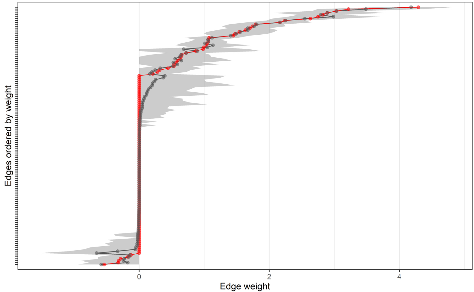

The social and financial support group (red) consists of four nodes that represent unemployment (FinSup), debts and severe social problems (SocRes and SocSpec). Financial support is connected to each of the other nodes in the group and it is the only node in the graph with connections to nodes in all five groups, although the edge with public transport (PubTr) in the disability support group is negative. All four social and financial support nodes are connected to general social care (GCsoc) and three of them are also linked to general youth care (GCyth). The social and financial support group is unlike other groups in the graph, which all broadly correspond to recognisable types of households and associated problems, for example: Physical disabilities, elderly with geriatric problems, adults in need of light support for independent living, and households with children or young adults facing youth-related problems. The social and financial support group, in contrast, is linked both to (adult-oriented) support for independent living and to youth related problems. The strongest of these links are the edges that connect financial support (FinSup) and debts to both forms of general care (GCsoc and GCyth).

The bootstrapped confidence intervals for all $136$ possible edges are displayed in Fig. 4, together with the estimated edge weights from the original sample (red) and the bootstrap means (black). The names of the corresponding node pairs are not shown here for the sake of readability. Overall, the sample weights and the bootstrap means match each other closely. The correlation between them is $0.99$ and the average difference between the estimates and the bootstrap means is very small ( $0.05$ ). All edges with confidence intervals that do not include $0$ are present in the graph. Edges that were excluded from the graph all are relatively weak with bootstrapped means well below $1.0$ .

4.2 Centrality

Figure 5 shows the standardized strength centrality scores of all nodes. General social care (GCsoc), public transport (PubTr), basic housekeeping (HKbasic) and general youth care (GCyht) highest strength scores. All of these nodes have in common that they are strongly connected to nodes within their own group and have relatively strong connections to nodes of other groups as well. If the public services in our data can be interpreted as proxies for underlying problems, then these centrality scores may provide clues to which problems are most likely to negatively impact other areas and may therefore be of interest to social policy makers who seek to improve prevention or social support efforts.

The high rankings of both general care (GCsoc and GCyth) forms reflect the role these services play in managing the involvement of specialised care, as well as the fact that households dealing with social and mental health issues are more likely to experience financial distress. Public transport (PubTr) and basic housekeeping (HKbasic) are connected to geriatric problems, but not necessarily to severe physical disabilities. The high strength scores of these nodes are caused by connections to services that are associated with physical disabilities. Hypothetically, this connection may be caused by the worsening of geriatric problems over time. Public transport and basic housekeeping could be early indicators of future requests for additional disability support; information like this may be of use to social policy makers, for example with regard to prognosticating future demand for social services.

Figure 5.

Centrality indices: Strength, closeness and betweenness.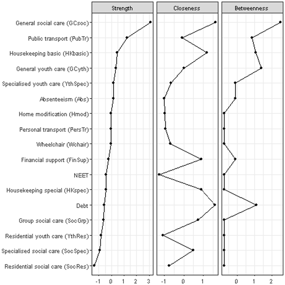

Figure 6.

Correlation of strength centrality indices from smaller bootstrapped samples with the original sample strength index. The lower limit of the CI (shaded area) reaches 0.7 for bootstrapped samples of 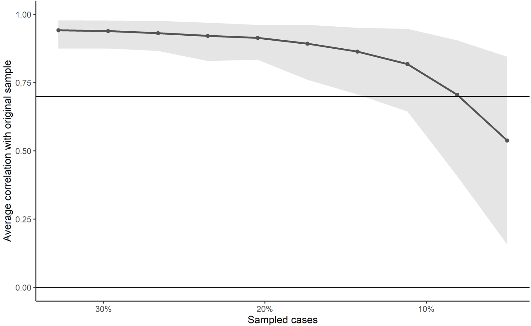$14\%$ of the original sample size.

The centrality indices for closeness and betweenness are also shown in Fig. 5. The scores for the debts node are the most strikingly different from the strength centrality score. This relatively weakly connected node has the highest closeness score and the third highest betweenness score. While there is no established way to interpret these indices, this does reinforce the qualitative observation that debts and financial support (FinSup) have a special position in the graph, as these link the youth-related nodes to nodes that involve social care. Another interesting observation on closeness and betweenness is that while absenteeism (Abs) has a relatively high strength centrality score, the closeness and betweenness scores are much lower. Since the high strength of absenteeism largely results from the strong link with NEET, closeness and betweenness seem to better reflect the position of absenteeism than strength centrality, or at least they provide a more nuanced picture than strength centrality by itself.

The stability of the strength centrality index was tested over $2,500$ bootstrapped samples with $m$ -out-of- $n$ case dropping and the recommended correlation threshold of $0.7$ [57]. The correlations of the bootstrap samples are summarised in Fig. 6. The centrality stability for Strength centrality $CS(cor=0.7)=0.86$ . In other words, the correlation between the original strength index and indices based on sub-samples will remain $0.7$ or higher with $95\%$ confidence as long as no more than $86\%$ of the cases are dropped from the sample. This is considerably better than the recommended minimum ( $0.25$ ) and preferred ( $0.5)$ cut-off scores based on simulation studies. The strength centrality index can be considered to be highly stable.

4.3 Classification performance

The graph can be used to predict node states if the states of neighbouring nodes are given. As discussed in Section 2.1, the conditional probability function for a single node is logistic. However, even when this fact is used in MRF estimation, the estimates from the MRF are not necessarily equal to those from logistic regression, due to the model restriction that edge weights (regression coefficients) should be equal for both nodes in each pair. Therefore, a difference in performance between the MRF logistic models and separately fitted logistic regression models is likely.

The graphical model was used to predict node outcomes on the test data. A univariate logistic regression model was fitted for each node, using all other nodes as predictor variables. The univariate logistic regression models were then used to predict node outcomes for comparison against the graphical model. The classification performance as measured by True positive rate (TPR/Sensitivity/Recall), Precision and F1-scores [84, 85] is shown in Table 2.

Table 2
Classification metrics of the graph and univariate logistic regression models (LR) compared: TRP (True positive rate), Prec (Precison) and F1 (F1 score)

Node	TPR: Graph	TPR: LR	Prec: Graph	Prec: LR	F1: Graph	F1: LR
Debt	0.00	0.02	0.00	0.38	0.00	0.04
FinSup	0.16	0.17	0.62	0.63	0.25	0.27
Abs	0.14	0.16	0.89	0.78	0.24	0.26
NEET	0.00	0.01	0.00	1.00	0.00	0.03
GCyth	0.21	0.23	0.73	0.71	0.32	0.35
GCsoc	0.48	0.53	0.78	0.77	0.59	0.63
Hmod	0.22	0.29	0.59	0.59	0.32	0.39
HKbasic	0.54	0.51	0.66	0.71	0.59	0.60
HKspec	0.00	0.07	0.00	0.73	0.00	0.13
PersTr	0.19	0.26	0.62	0.59	0.29	0.36
PubTr	0.45	0.45	0.71	0.71	0.55	0.56
SocGrp	0.00	0.00	0.00	0.00	0.00	0.00
SocRes	0.00	0.00	0.00	0.00	0.00	0.00
SocSpec	0.00	0.00	0.00	0.00	0.00	0.00
Wchair	0.25	0.25	0.56	0.57	0.35	0.35
YthSpec	0.13	0.14	0.76	0.73	0.22	0.23
YthRes	0.00	0.07	0.00	0.57	0.00	0.13
Mean score	0.16	0.17	0.41	0.56	0.22	0.25

As is to be expected with variables that have severe class imbalances (see Table 1), in absolute terms the graphical model struggles to correctly classify cases across all nodes. The mean scores reflect the poor overall performance of the model with TRP $=$ 0.16, Precision $=$ 0.41 and F1-score $=$ 0.22. However, the univariate logistic regression models did not fare much better (TPR $=$ 0.17; Precision $=$ 0.56; F1-score $=$ 0.25). Of these measures, Precision was most notably better for the logistic regression models, while the more crucial TPR was only slightly higher. For the nodes Debt, NEET and Residential youth care (ResYth) the graphical model failed to predict any positive cases, while the univariate models succeeded in identifying at least some positive cases. The logistic regression model for NEET has an optimal score for Precision. The model predicted only a single case of NEET, which happened to be correct. However, it failed to identify any other positive cases, which is reflected by a TPR of $0.01$ .

5. Discussion and conclusion

The aim of this article was to demonstrate how undirected models can be valuable to social policy by applying them to linked administrative data. The resulting graph provides an intuitively understandable overview of how 17 municipal social services at household level are related. The graph is readily interpreted, yet contains a large amount of information. This ability to present complexity in a way that makes it easy to interpret can by itself be regarded as a valuable result.

The high degree of centrality stability in our model indicates that the structural features of the graph can reliably be found in random subsets of the data. The estimated structure, therefore, cannot be attributed to mere random noise. General patterns of node interrelation correspond to prior knowledge and expectations. The groups that were discovered with a community-finding algorithm roughly match the a priori grouping. The few nodes that were found by the walktrap algorithm to be in different groups – basic housekeeping and specialised and residential social care – were all strongly connected to their expected groups. Overall, these results increase our confidence that the remaining findings also represent real-world phenomena.

Several of our findings from the graph result from the organization of social care in Netherlands. For example, “general social care” is a service that is administratively intended to play a central role in the further referral and provision of other social care, and this node is indeed found to have the highest centrality in the graph. While it could be said that such findings could have been predicted in advance based on the administrative organization of social services, administrative realities do not always match the reality on the ground.

Furthermore, several of our findings are potentially useful from a substantive point of view. Most striking is the high betweenness of financial hardship variables (central red nodes in Fig. 3). We conclude that these variables may play a pivotal role in conducting the “flow” between, on the one hand, disability-related and light social care problems such as a need for special housekeeping, and, on the other hand, youth care and educational problems. The estimated graph predicts that intervening on financial hardship problems makes these two groups of variables almost independent. In other words, vulnerability to financial problems is a common denominator for households with either of these different types of problems. We also note that, on a smaller scale, absenteeism plays a similar role in connecting NEET to the broader network.

Our work also has a number of limitations that warrant further study.

First, we have used observational, cross-sectional data to infer something of the (unknown) causal connections between variables. To some extent this drawback was mitigated by using undirected models, which do not attempt to infer causal direction. However, some caveats do remain with this approach. Temporal psychological networks have been used to predict key psycho-pathological transition events in patients with a history of depression, by applying the concept of critical slowing down before phase transitions that is used in research on climate and ecosystems, and recently also in medical and psychological research [62, 86]. Introducing time based on registration data into a graphical model will provide many new challenges. The added complexities that come with time and registration data were the reason not to include time in this study. In future work, we hope to leverage the fact that our full data set also contains longitudinal information.

Second, although administrative registers in the Netherlands have as an advantage that they contain all residents in the municipality at hand, a disadvantage is that the variables observed are simply those resulting from the administrative process, and were not necessarily intended for social research. In general this may result in problems of measurement error and validity [87, 88, 89].

Specifically, in our analysis the ideal measurements would have been those of social problems, but we have observed social services. While these two are very closely related, they are not identical, and we were only able to take account of these differences in the interpretation of our results through substantial knowledge of the basic administrative processes behind the generation of these registers. We caution others interested in applying our approach to administrative registers that involvement of a party intimately familiar with these processes is crucial.

A third limitation of our approach is that we were unable to obtain interpretable results using larger $n>$ 100,000 household datasets, and, furthermore, measures introduced in the psychological literature to evaluate stability and precision of the model estimates broke down at these sample sizes due to increased computation times. Because we believe assessment of the uncertainties is essential, we chose to reduce the sample size to $6,000$ , still well above the largest sample size at which MRFs were applied in social research to our knowledge. Future research might leverage more efficient computational methods or analytical results to achieve uncertainty quantification.

Fourth, classification performance by the graphical model, as well as logistic regression, was rather poor in an absolute sense. Classification will always be a challenge for any model due to the class imbalances present in all variables. Because our aim was to interpret the graph, rather than optimize prediction, no specific actions were taken to optimize the model for predictive purposes as is common in machine learning approaches. This means that model performance in the predictive sense could likely be improved. Exceptional model mining [90] might prove useful to identify subgroups with less class imbalance for which group-specific graphical models with atypical features can be estimated. Ultimately, in some cases it may simply be enough if the model can accurately identify cases with an increased risk of specific problems. For example, a municipality could include a question to screen for financial problems while offering certain other social services. This requires very little effort and it can be done unobtrusively, so there is no risk or cost associated with false positives.

Fifth, we did not examine individual differences in graph structure. The households in the sample consist of many different subgroups that are likely to have different needs of social services. For example, households without any children or young adults will not encounter youth care or educational support services; certain services are primarily requested by elderly citizens; and young single males and single parents are among households with the highest risk of problem debts. Group comparison is not a straightforward matter with the graphical model we used, however. For one, the number of observations in each group influences the size of regularisation parameter $\lambda$ (Eq. (4)) and the value of the extended BIC (Eq. (5)), so that graphs can only be compared directly if the sample sizes the groups are equal. We hope to explore group comparison in future studies. Conditional random fields may be suitable to include variables predictive of such group membership, such as age and household type, in the graphical model.

Sixth, we did not compare graphs obtained with different parameters or different methods of model selection. Instead we only used the eLasso method with hyper-parameter $\gamma=0.25$ as recommended by the authors of the method [53]. As a consequence, we do not know whether better models could have been found by using different values for $\gamma$ or with alternatives to the extended BIC [77, 91] for model selection. For model comparison purposes, in addition to classification performance as described in 2, it is possible to compute the joint likelihood in Eq. (1) for these models; this equation also yields the $G^{2}$ score traditionally used in the log-linear modelling literature for comparing models [65].

In conclusion, household poverty and debt, while complex social problems, can be better understood within a “network” of interrelated variables. We accomplished this by applying Markov random fields to linked administrative data, an approach that we believe can bring fruitful further insights for social policy and intervention. We hope other researchers will find the approach presented here equally useful when applied to other social problems.

Footnotes

Acknowledgments

We thank the municipality of Utrecht for creating the necessary conditions to study their data in compliance with Dutch General Data Protection Regulation.

Supplementary data

The supplementary files are available to download from https://dx-doi-org.web.bisu.edu.cn/10.3233/SJI-230028.

References

Balmer

Pleasence

Buck

Walker

. Worried Sick: The Experience of Debt Problems and their Relationship with Health, Illness and Disability. Social Policy and Society. 2006; 5: 39-51. doi: 10.1017/S147474640500271X.

Barba

Pivetti

. Rising Household Debt: Its Causes and Macroeconomic Implications-A Long-Period Analysis. Cambridge Journal of Economics. 2009; 33: 113-37. doi: 10.1093/cje/ben030.

Carter

Blakely

Collings

Gunasekara

Richardson

. What is the association between wealth and mental health? Journal of Epidemiology & Community Health. 2009; 63: 221-6. doi: 10.1136/jech.2008.079483.

Cuesta

Cotini

Herrarte

. The socioeconomic gradient in health: How important is material deprivation? The Journal of Economic Inequality. 2013; 12. doi: 10.1007/s10888-013-9248-5.

Hayhoe

Cho

Devaney

Worthy

Kim

Gorham

. How Do Distrust and Anxiety Affect Saving Behavior? Family and Consumer Sciences Research Journal. 2012 Sep; 41. doi: 10.1111/j.1552-3934.2012.02129.x.

Kamleitner

Hoelzl

Kirchler

. Credit use: Psychological perspectives on a multifaceted phenomenon. International Journal of Psychology: Journal International de Psychologie. 2012 Feb; 47: 1-27. doi: 10.1080/00207594.2011.628674.

Legge

Heynes

. Beyond reasonable debt: A background report on the indebtedness of New Zealand families. Social Policy Journal of New Zealand 2009 Jun; 35.

Leigh

Jencks

Smeeding

. The Oxford Handbook of Economic In- equality (2009). Oxford University Press, 2011; Chap. Health and Economic Inequality.

Lerner

Weber

. The Financial Costs of Sadness. Psychological Science. 2012 Nov; 24. doi: 10.1177/0956797612450302.

10.

McNair

Summers

Bruin

W Bruine de

Ranyard

. Individual-level factors predicting consumer financial behavior at a time of high pressure. Personality and Individual Differences. 2016 Sep; 99: 211-6. doi: 10.1016/j.paid.2016.05.034.

11.

Pickett

Wilkinson

. Income Inequality and Health: A Causal Review. Social Science & Medicine (1982). 2014 Dec; 128. doi: 10.1016/j.socscimed.2014.12.031.

12.

Oksanen

Aaltonen

Rantala

. Social Determinants of Debt Problems in a Nordic Welfare State: a Finnish Register-Based Study. Journal of Consumer Policy. 2015 May; 38. doi: 10.1007/s10603-015-9294-4.

13.

Oksanen

Aaltonen

Rantala

. Debt problems and life transitions: a register-based panel study of Finnish young people. Journal of Youth Studies. 2016; 19: 1184-203. doi: 10.1080/13676261.2016.1145638.

14.

Webley

Nyhus

. Life-Cycle and Dispositional Routes into Problem Debt. British Journal of Psychology (London, England: 1953). 2001 Sep; 92: 423-46. doi: 10.1348/000712601162275.

15.

Brady

Finnigan

Huübgen

. Rethinking the Risks of Poverty: A Framework for Analyzing Prevalences and Penalties. American Journal of Sociology. 2017; 123: 740-86. doi: 10.1086/693678.

16.

Livingstone

Lunt

. Predicting personal debt and debt repayment: Psy-chological, social and economic determinants. Journal of Economic Psychology. 1992; 13: 111-34. doi: 10.1016/0167-4870(92)90055-C.

17.

Schicks

. Over-Indebtedness in Microfinance – An Empirical Analysis of Related Factors on the Borrower Level. World Development. 2014; 54: 301-24.

18.

Brady

. Theories of the Causes of Poverty. Annual Review of Sociology. 2019; 45: 155-75.

19.

Schicks

. The Definition and Causes of Microfinance Over-Indebtedness: A Customer Protection Point of View. Oxford Development Studies. 2013 Aug; 41. doi: 10.1080/13600818.2013.778237.

20.

Richardson

Elliott

Roberts

. The relationship between personal unsecured debt and mental and physical health: A systematic review and metaanalysis. Clinical Psychology Review. 2013 Sep; 33: 1148-62. doi: 10.1016/j.cpr.2013.08.009.

21.

Avendano

Glymour

. Stroke Disparities in Older Americans Is Wealth a More Powerful Indicator of Risk Than Income and Education? Stroke; a Journal of Cerebral Circulation. 2008; 39: 1533-40. doi: 10.1161/STROKEAHA.107.490383.

22.

Averett

Smith

. Financial hardship and obesity. Economics & Human Biology. 2014; 15: 201-12. doi: 10.1016/j.ehb.2013.12.004.

23.

Wilkinson

Pickett

. The Spirit Level: Why Greater Equality Makes Societies Stronger. Bloomsbury Publishing, 2010.

24.

Bridges

Disney

. Debt and depression. Journal of Health Economics. 2010; 29: 388-403. doi: 10.1016/j.jhealeco.2010.02.003.

25.

Brown

Taylor

Price

. Debt and Distress: Evaluating the Psychological Cost of Credit. Journal of Economic Psychology. 2005; 26: 642-63. doi: 10.1016/j.joep.2005.01.002.

26.

Meltzer

Bebbington

Brugha

Farrell

Jenkins

. The relationship between personal debt and specific common mental disorders. European Journal of Public Health. 2012 Mar; 23. doi: 10.1093/eurpub/cks021.

27.

Pevalin

. Housing repossessions, evictions and common mental illness in the UK: results from a household panel study. Journal of Epidemiology & Community Health. 2009; 63: 949-51. doi: 10.1136/jech.2008.083477.

28.

Taylor

Pevalin

Todd

. The psychological costs of unsustainable housing commitments. Psychological Medicine. 2007 Aug; 37: 1027-36. doi: 10.1017/.S0033291706009767.

29.

Kim

Garman

. Financial Stress, Pay Satisfaction and Workplace Performance. Compensation & Benefits Review. 2004 Feb; 36: 69-76. doi: 10.1177/0886368703261215.

30.

Aittomaäki

Martikainen

Laaksonen

Lahelma

Rahkonen

. The associations of household wealth and income with self-rated health – A study on economic advantage in middle-aged Finnish men and women. Social Science & Medicine. 2010; 71: 1018-1026. doi: 10.1016/j.socscimed.2010.05.040.

31.

Morris

Sutton

Gravelle

. Inequity and inequality in the use of health care in England: An empirical investigation. Social Science & Medicine (1982). 2005 Apr; 60: 1251-66. doi: 10.1016/j.socscimed.2004.07.016.

32.

Mullainathan

Shafir

. Scarcity: Why Having Too Little Means so Much. New York: Times Books, Henry Holt and Company, 2013.

33.

Taylor

. Measuring Financial Capability and its Determinants Using Survey Data. Social Indicators Research 2011 Jun; 102: 297-314. doi: 10.1007/s11205-010-9681-9.

34.

Turunen

Hiilamo

. Health effects of indebtedness: A systematic review. BMC Public Health. 2014 May; 14: 489. doi: 10.1186/1471-2458-14-489.

35.

Barrett

Garg

Mcbride

. Well-Being Dynamics and Poverty Traps. Annual Review of Resource Economics. 2016; 8. doi: 10.1146/annurev-resource-100815-095235.

36.

Haushofer

Fehr

. On the psychology of poverty. Science (New York, N.Y.) 2014 May; 344: 862-7. doi: 10.1126/science.1232491.

37.

Ridley

Rao

Schilbach

Patel

. Poverty depression, and anxiety: Causal evidence and mechanisms. Science. 2020; 370. doi: 10.1126/science.aay0214.

38.

McGrath

. Conceptual Complexity and Construct Validity. Journal of Personality Assessment. 2005 Nov; 85: 112-24.

39.

Cramer

Waldorp

Maas

Borsboom

. Comorbidity: A network perspective. The Behavioral and Brain Sciences. 2010 Jun; 33: 137-50, discussion 150. doi: 10.1017/S0140525X09991567.

40.

Boccaletti

Latora

Moreno

Chavez

Hwang

. Complex networks: Structure and dynamics. Physics Reports. 2006; 424: 175-308. doi: 10.1016/j.physrep.2005.10.009.

41.

Goodman

. The Multivariate Analysis of Qualitative Data: Interactions among Multiple Classifications. Journal of the American Statistical Association. 1970; 65: 226-56. doi: 10.1080/01621459.1970.10481076.

42.

Koller

Friedman

. Probabilistic Graphical Models: Principles and Techniques. MIT Press. 2009; 13: 103-56.

43.

Pescosolido

Kelley

. Confronting Sociological Theory with Data: Regression Analysis, Goodman’s Log-Linear Models and Comparative Research. Sociology. 1983; 17: 359-79. doi: 10.1177/0038038583017003003.

44.

Fienberg

. Contingency Tables and Log-Linear Models: Basic Results and New Developments. Journal of the American Statistical Association. 2000; 95: 643-7. doi: 10.1080/01621459.2000.10474242.

45.

Wright

. Correlation and causation. Journal of Agricultural Research. 1921; 20: 557-85.

46.

Bollen

. Structural Equations with Latent Variables. John Wiley & Sons, Ltd, 1989, doi: 10.1002/9781118619179.fmatter.

47.

Kesteren van

Oberski

. Flexible Extensions to Structural Equation Models Using Computation Graphs. Structural Equation Modeling: A Multidisciplinary Journal. 2022; 29: 233-47. doi: 10.1080/10705511.2021.1971527.

48.

Pearl

. Causality: Models, Reasoning and Inference. 2nd. USA: Cambridge University Press, 2009.

49.

Vander Weele

. Explanation in causal inference: methods for mediation and interaction. Oxford University Press, 2015.

50.

Gibbs

. Elementary Principles in Statistical Mechanics, Developed with Especial Reference to the Rational Foundation of Thermodynamics. Dover Publications, 1902.

51.

Ising

. Beitrag zur Theorie des Ferromagnetismus. Zeitschrift fuür Physik. 1925; 31(1): 253-8.

52.

Murphy

. Machine learning: a probabilistic perspective. MIT press, 2012.

53.

Borkulo van

Borsboom

Epskamp

Blanken

Boschloo

Schoevers

Waldorp

. A new method for constructing networks from binary data. Scientific Reports. 2014 Aug; 4: 5918. doi: 10.1038/srep05918.

54.

Borsboom

Cramer

. Network Analysis: An Integrative Approach to the Structure of Psychopathology. Annual Review of Clinical Psychology. 2013; 9: 91-121. doi: 10.1146/annurev-clinpsy-050212-185608.

55.

Cramer

AOJ

Borsboom

. Problems Attract Problems: A Network Perspective on Mental Disorders. Emerging Trends in the Social and Behavioral Sciences American Cancer Society. 2015; 1-15. doi: 10.1002/.9781118900772.etrds0264.

56.

Dalege

Borsboom

Harreveld van

Maas

. Network Analysis on Attitudes: A Brief Tutorial. Social Psychological and Personality Science. 2017; 8. doi: 10.1177/1948550617709827.

57.

Epskamp

Borsboom

Fried

. Estimating Psychological Networks and their Accuracy: a Tutorial Paper. Behavior Research Methods. 2016a; 50. doi: 10.3758/s13428-017-0862-1.

58.

Epskamp

Rhemtulla

Borsboom

. Generalized Network Psychometrics: Combining Network and Latent Variable Models. Psychometrika. 2016b; 82. doi: 10.1007/s11336-017-9557-x.

59.

Fried

Eidhof

Palic

Costantini

Dijk

Bockting

Engelhard

Armour

Nielsen

Karstoft

. Replicability and Generalizability of Posttraumatic Stress Disorder (PTSD) Networks: A Cross-Cultural Multisite Study of PTSD Symptoms in Four Trauma Patient Samples. Clinical Psychological Science. 2018 Jan; 6: 216770261774509. doi: 10.1177/2167702617745092.

60.

Haslbeck

Fried

. How predictable are symptoms in psychopathological networks? A reanalysis of 18 published datasets. Psychological Medicine. 2017 Jun; 47: 1-10. doi: 10.1017/S0033291717001258.

61.

Haslbeck

Waldorp

. mgm: Estimating Time-Varying Mixed Graphical Models in High-Dimensional Data. Journal of Statistical Software. 2020 Apr; 93. doi: 10.18637/jss.v093.i08.

62.

Olde Rikkert

MGM

Dakos

Buchman

Boer

Glass

Cramer

AOJ

Levin

Nes van

Sugihara

Ferrari

Tolner

Leemput van de

Lagro

Melis

Scheffer

. Slowing Down of Recovery as Generic Risk Marker for Acute Severity Transitions in Chronic Diseases. Journal of Personality Assessment. 2016 Mar; 44.

63.

Bringmann

Elmer

Epskamp

Krause

Schoch

Wichers

Wigman

Snippe

. What Do Centrality Measures Measure in Psychological Networks? Journal of Abnormal Psychology. 2019 Jul; 128. doi: 10.1037/abn0000446.

64.

Haberman

. Analysis of Qualitative Data, Volume 1. Academic Press, 1978. doi: 10.1016/B978-0-12-312501-9.50010-9.

65.

Agresti

Caffo

. Measures of relative model fit. Computational Statistics & Data Analysis. 2002; 39: 127-36. doi: 10.1016/S0167-9473(01)00054-8.

66.

Burger

Isvoranu

Lunansky

Haslbeck

Epskamp

Hoekstra

Fried

Borsboom

Blanken

. Reporting standards for psychological network analyses in cross-sectional data. Psychological Methods. 2022 Apr. doi: 10.1037/.met0000471.

67.

Clifford

. Markov random fields in statistics. Disorder in physical systems: A volume in honour of John M. Hammersley. 1990; 19-32.

68.

Anandkumar

Tan

VYF

Huang

Willsky

. High-dimensional structure estimation in Ising models: Local separation criterion. The Annals of Statistics. 2012; 40: 1346-1375. doi: 10.1214/12-AOS1009.

69.

Bogdanov

Mossel

Vadhan

. The Complexity of Distinguishing Markov Random Fields. Approximation, Randomization and Combinatorial Optimization. Algorithms and Techniques Ed. by Goel A, Jansen K, Rolim JDP, and Rubinfeld R. Berlin, Heidelberg: Springer Berlin Heidelberg, 2008; 331-42.

70.

Sanghavi

Dimakis

. Sparse logistic regression learns all discrete pairwise graphical models. Advances in Neural Information Processing Systems. 2019; 32: 8071-81.

71.

Besag

. Nearest-Neighbour Systems and the Auto-Logistic Model for Binary Data. Journal of the Royal Statistical Society Series B (Methodological). 1972; 34: 75-83.

72.

Besag

. Spatial Interaction and the Statistical Analysis of Lattice Systems. Journal of the Royal Statistical Society Series B (Methodological). 1974; 36: 192-236.

73.

Tibshirani

. Regression Shrinkage and Selection Via the Lasso. Journal of the Royal Statistical Society: Series B (Methodological). 1996; 58: 267-88. doi: 10.1111/j.2517-6161.1996.tb02080.x.

74.

Ravikumar

Wainwright

Lafferty

. High-dimensional Ising model selection usingregularized logistic regression. Annals of Statistics ANN STATIST. 2010 Jun; 38. doi: 10.1214/09-AOS691.

75.

Meinshausen

Buühlmann

. High dimensional graphs and variable selection with the LASSO. The Annals of Statistics. 2006 Sep; 34. doi: 10.1214/009053606000000281.

76.

Friedman

Hastie

Tibshirani

. Regularization Paths for Generalized Linear Models via Coordinate Descent. Journal of Statistical Software. 2010; 33: 1-22.

77.

Chen

. Extended Bayesian information critera for model selection with large model spaces. Biometrika. 2008 Feb; 95: 759-71. doi: 10.1093/biomet/asn034.

78.

Petitjean

Webb

Nicholson

. Scaling Log-Linear Analysis to High-Dimensional Data. 2013 IEEE 13th International Conference on Data Mining. 2013; 597-606. doi: 10.1109/ICDM.2013.17.

79.

Epskamp

Borkulo van

Veen van der

Servaas

Isvoranu

Riese

Cramer

AOJ

. Personalized Network Modeling in Psychopathology: The Importance of Contemporaneous and Temporal Connections. Clinical Psychological Science. 2018; 6: 416-27. doi: 10.1177/2167702617744325.

80.

Pons

Latapy

. Computing Communities in Large Networks Using Ran- dom Walks. Computer and Information Sciences ISCIS 2005. Ed. by Yolum p, Güngör T, Gürgen F, and Özturan C. Berlin, Heidelberg: Springer Berlin Heidelberg, 2005; 284-93.

81.

Pons

Latapy

. Computing Communities in Large Networks Using Random Walks. J. Graph Algorithms Appl. 2006 Jan; 10: 191-218. doi: 10.7155/jgaa.00124.

82.

Yang

Algesheimer

Tessone

. A Comparative Analysis of Community Detection Algorithms on Artificial Networks. Scientific Reports. 2016; 6(1).

83.

Fruchterman

Reingold

. Graph drawing by force-directed placement. Software: Practice and Experience. 1991; 21: 1129-64.

84.

Chinchor

. MUC-4 Evaluation Metrics. Proceedings of the 4th; Conference on Message Understanding McLean, Virginia: Association for Computational Linguistics, 1992. doi: 10.3115/1072064.1072067.

85.

Rijsbergen

CJV

. Information Retrieval. 2nd. USA Butter- worth-Heinemann, 1979.

86.

Leemput van de

Wichers

Cramer

Borsboom

Tuerlinckx

Kuppens

Nes van

Viechtbauer

Giltay

Aggen

, et al. Critical slowing down as early warning for the onset and termination of depression. Proceedings of the National Academy of Sciences. 2014; 111: 87-92.

87.

Oberski

. Estimating error rates in an administrative register and survey questions using a latent class model. Total survey error in practice: improving quality in the era of big data Ed. by Biemer PP, Leeuw EDD, Eckman S, Edwards B, Kreuter F, Lyberg LE, Tucker C, and West BT. New York: Wiley, 2016.

88.

Hand

. Statistical challenges of administrative and transaction data. Journal of the Royal Statistical Society: Series A (Statistics in Society). 2018; 181: 555-605. doi: 10.1111/rssa.12315.

89.

Pankowska

Pavlopoulos

Bakker

Oberski

. Reconciliation of inconsistent data sources using hidden Markov models. Statistical Journal of the IAOS. 2020; 36: 1261-79.

90.

Duivesteijn

Feelders

Knobbe

. Exceptional model mining. Data Mining and Knowledge Discovery. 2016; 30: 47-98.

91.

Chen

. Extended BIC for small-n-large-p sparse GLM. Statistica Sinica. 2012 Apr; 22. doi: 10.5705/ss.2010.216.

Understanding financial distress by using Markov random fields on linked administrative data

Abstract

Keywords

1. Introduction

2.1 Model definition

2.3.1 Edge-weight accuracy and centrality stability

2.4 Model interpretation

2.4.1 Node centrality measures

3. Data

3.1 Data collection and preparation

3.1.1 Variables and descriptives

Table 1 Proportions of (semi-)public service use. High refers to High social housing ( n = 6 , 848 ), Other to Other neighbourhoods ( n = 117 , 544 )

Table 2 Classification metrics of the graph and univariate logistic regression models (LR) compared: TRP (True positive rate), Prec (Precison) and F1 (F1 score)

Footnotes

Acknowledgments

Supplementary data

References

Table 1
Proportions of (semi-)public service use. High refers to High social housing ( $n=6,848$ ), Other to Other neighbourhoods ( $n=117,544$ )

Table 2
Classification metrics of the graph and univariate logistic regression models (LR) compared: TRP (True positive rate), Prec (Precison) and F1 (F1 score)