Small data estimation for binary variables with big data: A comparison of calibrated nearest neighbour and hierarchical Bayes methods of estimation

Abstract

A recent application in machine learning has introduced a novel approach, complemented by big data sources, aimed at providing precise estimates for small geographical areas. This method employs a dual strategy: (a) hybrid estimation, involving the integration of big data sources with imputed values derived from $K$ nearest neighbours (KNN) to address missing target variable values from the big data source; and (b) calibration of the collective sum of small area estimates to an independent yet efficient national total. Evaluating its efficacy using simulated data from the 2016 Australian population census, the calibrated KNN (CKNN) method demonstrated superior performance compared to the Fay-Herriot method based on area-level covariates.

This paper enhances the comparative analysis by contrasting the CKNN method with a hierarchical Bayes method using the logit-normal model (LN) relevant for binary data. Broadly speaking, the LN method can be viewed as the Bayesian equivalent of Battese-Harter-Fuller (BHF) method, which incorporates unit-level covariates. Our results demonstrate the CKNN method’s superiority over the LN method. However, the application of hybrid estimation to the LN method significantly diminishes this superiority. Although CKNN estimates maintain better precision, they are not as accurate as the estimates from the hybridized LN method.

Keywords

Calibration KNN small area estimation

1. Introduction

The estimation of variables in small geographic areas, known as small area estimation (SAE), is recognized as a crucial yet inadequately addressed requirement by national statistical offices (NSOs) and is particularly pertinent to the needs of statistical users. While “small areas” typically refers to sub-national or local geographical regions, it is important to note that the same principles and methodologies for national estimates are equally applicable to the estimation for small population groups.

The unmet demand for SAE arises due to the inherent limitations of direct estimates for small areas, primarily stemming from the challenges associated with small, or non-existent sample sizes, leading to substantial sampling errors. To overcome this hurdle, NSOs employ a “model-based approach,” utilizing statistical models to leverage information and enhance estimation accuracy across areas [1, 2], over time [3], or resort to synthetic estimation techniques [4]. The Fay and Herriot (FH) and Battese, Harper and Fuller (BHF) models, which use area-level and unit-level covariates respectively, are commonly used by NSOs and are considered to be the industry-standards for SAE.

For a comprehensive understanding of the various methodologies employed in small area estimation, one may refer to the extensive literature, including [5, 6, 7, 8, 9, 10, 11, 12, 13, 14].

The FH model enhances the precision of SAE by “borrowing” strength across areas, employing what is known as “linking” models – refer to, for instance, equation 4.2.1 of [14]. This improvement is achieved by assuming shared regression coefficients in the linking model for area totals. By amalgamating the sampling error model (equation 4.2.3 of [14]) with the linking model, a mixed linear model (equation 4.2.5 of [14]) for the survey estimates (which are appropriately weighted) of the areas is derived. Subsequently, model parameters are estimated through this combined framework. Empirical Best Linear Unbiased Predictors (EBLUPs) for the small areas are then computed by plugging the estimated parameters into the mixed linear model, along with the area-level covariates.

The BHF builds upon the aforementioned concept by employing a mixed linear model, focusing not on the survey estimates of the areas, but on the survey units directly. An essential condition for implementing the BHF model is the presence of unit-level covariates, not only for the observed units in the survey sample but for the entire population. Through simulation studies [15, 16], it has been demonstrated that SAEs derived from BHF models surpass FH estimates in terms of precision and are less susceptible to bias. This superiority arises from the more granular information available in unit-level covariates, providing more informative estimation compared to the FH models operating at the area level.

In this paper, we employ the LN model instead of the BHF model for comparison. The LN model can be considered as the Bayesian equivalent to the BHF model as it also uses unit covariates for prediction, offering a compatible framework for our analysis. The principal reason for choosing the LN model instead of the BHF model is that, using Monte Carlo Markov Chain (MCMC) for computations, the LN model facilitates more efficient number-crunching compared to the BHF model.

The subsequent Sections of this paper are organized as follows. Section 2 provides an overview of the calibrated KNN (CKNN) methodology, elucidating its application in generating small area estimates and the associated computation of mean squared errors (MSE). Moving forward, Section 3 summarises the outcomes of a comparative analysis between CKNN estimates and those derived from the FH method. Section 4 reports the findings of a parallel assessment, contrasting CKNN estimates against both LN estimates and hybridized LN estimates. Our concluding remarks are presented in Section 5.

2. Harnessing big data for SAE

As big data gains prominence [17, 18], the question arises: Can we unlock its potential for SAE? The response is in the affirmative, as demonstrated in [19]. Addressing the well-recognized under-coverage bias associated with relying solely on big data for SAE, [19] mitigates this limitation by mass imputing the missing data using survey data as donors and counters the constraints posed by the small sample size in SAE by complementing the imputed data with big data. This symbiotic relationship between the two data sources underscores their complementarity in achieving robust SAE outcomes.

In what follows, we provide a bird’s eye view of the methodology used in [19] for SAE with big data.

2.1 Notation and the underlying idea

Suppose we have a finite population, $U=\{1,\ldots$ , $N\}$ comprising $N$ units with the following values, $x_{i}$ and $y_{i}$ , $\forall i\in U$ , where $x_{i}$ is a vector of auxiliary variables and is fully observed, and $y_{i}$ is the variable of interest. We assume that $U=B\cup C$ , where $B$ , of size $N_{B}$ , comprises the labels of the big data set and $C$ , of size $N_{C}$ , is the complement of $B$ . We assume further that $y_{i},\forall i\in B$ , are observed without error. Finally, we also assume that we have a probability sample, $A\subset U$ , with known design weights of the sample, $d_{i}$ , $\forall i\in A.$ Thus we have the following data available to the analyst for SAE: (a) $(x_{i},y_{i}$ ) for $i\in B$ ; (b) $(d_{i},x_{i},y_{i})$ for $i\in A$ ; (c) $x_{i}\forall i\in C$ and (d) information on where these units are located in the small area. Finally, let $\delta_{i}$ denote the big data inclusion indicator which is 1 if unit $i\in B$ and 0 otherwise. We assume that (e) $\delta_{i}$ , $\forall i\in A$ , is fully observed. Note that $\delta_{i}=1$ is observed for $\forall i\in B.$ In addition, note that the case when $A$ is subject to nonresponse and $\delta_{i}$ not fully observed was addressed in [20] and [21] respectively and will not be repeated here.

Suppose further that $U=U_{1}\cup\ldots U_{m}\cup\ldots\cup U_{M},B=B_{1}\cup\ldots B_{m}\cup\ldots% \cup B_{M}$ and $C=C_{1}\cup\ldots C_{m}\cup\ldots\cup C_{M}$ and $A=A_{1}\cup\ldots A_{m}\cup\ldots\cup A_{M},$ where $U_{m}=B_{m}\cup C_{m}$ and $m$ denotes the $m^{th}$ small area. For SAE, we are interested to estimate $T_{m}=\sum_{i\in U_{m}}{y_{i}},m=1,\ldots,M$ . As $T_{m}=\sum_{i\in B_{m}}{y_{i}}+\sum_{i\in A_{m}\backslash B_{m}}{y_{i}}+\sum_{% i\in C_{m}\backslash A_{m}}{y_{i}}=T_{B_{m}}+T_{A_{m}\backslash B_{m}}+T_{C_{m% }\backslash A_{m}},$ and because $T_{B_{m}}$ and $T_{A_{m}\backslash B_{m}}$ are fully observed, the SAE problem boils down to estimating $T_{C_{m}\backslash A_{m}}$ , using the information available from (a) to (e) above. Let $\hat{T}_{C_{m}\backslash A_{m}}$ and $\hat{T}_{m}$ denote the estimate of $T_{C_{m}\backslash A_{m}}$ and $T_{m}$ respectively. Then

$\displaystyle\hat{T}_{m}=T_{B_{m}}+T_{A_{m}\backslash B_{m}}+\hat{T}_{C_{m}% \backslash A_{m}}.$

Denote the population total by $T=\sum_{m=1}^{M}{T_{m}}$ . [21] showed that the data integrator, perhaps better referred to as a hybrid estimator, $\hat{T}_{P}=\sum_{i\in U}{\delta_{i}y_{i}}+N_{C}\frac{\sum\limits_{i\in A}{d_{% i}(1-\delta_{i})y_{i}}}{\sum\limits_{i\in A}{d_{i}(1-\delta_{i})}},$ is equivalent to a generalised regression estimator and hence is approximately designed unbiased They also showed that when $W_{B}=N_{B}/N$ is sufficiently large, $\hat{T}_{P}$ is a more efficient estimator than $\hat{T}_{A}=N\sum_{i\in A}{y_{i}/n}$ , where $N_{B},N$ and $n$ denote the size of the Big Data, population and sample respectively. As $\hat{T}_{P}$ is an efficient estimator of the population total, [19] uses it to calibrate the imputes for the missing values in $C\backslash A,$ using a KNN algorithm with the donors coming from $D=A\cap C$ . In other words, $\hat{T}=\sum_{m=1}^{M}{\hat{T}_{.m}}=\hat{T}_{P},$ and the methodology is called the CKNN algorithm.

2.2 The KNN algorithm

For a description of the KNN algorithm, refer to [19] and the references therein. To ascertain the optimum number of nearest neighbours, $K$ the number, $p$ , and selection of the covariates in $x$ to be used in finding the nearest neighbours, the following two steps are applied [19]: (a) a grid search on all possible combinations of $K=1,\ldots,20$ and all combinations of the covariates from $p=1,\ldots,\dim(x)$ ; and (b) a 5-fold cross validation methodology. The objective is to identify the combination of $K$ , $p$ and the specific $p$ covariates that minimises the aggregated sum of absolute prediction errors across all the small areas from $m=1,\ldots,M$ .

Furthermore, [19] utilizes the HasD distance metric [19, 22] to find the nearest neighbours in $D$ , i.e. extending beyond the boundaries of the specific area to encompass the entire donor pool. This approach ensures a thorough exploration of potential matches, transcending the limitations of a localized focus. Conceptually, by sharing the donors across all areas in $D$ , this mirrors the assumption of shared regression coefficients used in the FH and BHF models. Finally, the HasD metric, which can handle continuous and multinomial data, is bounded between 0 and $p$ and offers the important characteristic of being scale invariant.

2.3 The CKNN algorithm

Let the subscript $m_{i}$ denote the $i^{th}$ unobserved unit in $E_{m}=C_{m}\backslash D_{m}$ and $y_{m_{i}(j)}$ , $j=1,\ldots,K$ be the $j t h$ nearest neighbour of $m_{i}$ , where $y_{m_{i}(j)}\in D.$ Denoting $\hat{T}_{E_{m}(j)}$ by $\sum_{m_{i}\in E_{m}}{y_{m_{i}(j)}}$ , an estimate for the population total in area $m$ from the $j^{th}$ donors is given by $\hat{T}_{m(j)}=T_{B_{m}}+T_{D_{m}}+\hat{T}_{E_{m}(j)}$ . In KNN, $\hat{T}_{\textit{KNNm}}=\frac{1}{K}\sum_{j=1}^{K}{\hat{T}_{m(j)}}$ . In CKNN, we define $\hat{T}_{\textit{CKNNm}}=\sum_{j=1}^{K}{w_{j}\hat{T}_{m(j)}},$ where $w_{j},j=1,\ldots,K$ is chosen to minimise $\sum_{j=1}^{K}{\frac{1}{K}}(Kw_{j}-1)^{2}$ subject to the following conditions: (a) $\sum_{j=1}^{K}{w_{j}=1}$ ; and (b) $\sum_{m=1}^{M}{\hat{T}_{\textit{CKNNm}}=}\hat{T}_{p}$ . The Chi-square minimisation criteria follows those of [23] and ensures that each $w_{j}$ , $j=1$ , $\ldots$ , $K$ , is as close as possible to $\frac{1}{K}$ whilst condition (b) ensures that entire sum of the estimates across all the areas is calibrated to the independent estimate of the overall population total, $\hat{T}_{p}$ . To simply notation, we shall henceforth use $\hat{T}_{m}$ to denote $\hat{T}_{\textit{CKNNm}}$ , and refer $\hat{T}_{m}$ as a CKNN estimate or a hybrid estimate signalling its combination of big data and survey data. The $w_{j},j=1,\ldots,K$ are also referred to as calibration weights.

For an analytic solution for the calibration weights, the reader is referred to the Lemma in [19].

2.4 Estimating the MSE of $\hat{T}_{m}$

The MSE of $\hat{T}_{m}$ can be decomposed into variance and a squared bias components as follows:

$\displaystyle\textit{MSE}(\hat{T}_{m})=E(\hat{T}_{m}-T_{m})^{2}$ $\displaystyle\quad=E\left\{{\hat{T}_{E_{m}}-E(\hat{T}_{E_{m}})}\right\}^{2}+% \left\{{E(\hat{T}_{E_{m}})-T_{E_{m}}}\right\}^{2}$ $\displaystyle\quad=E\left\{{\hat{T}_{E_{m}}-E(\hat{T}_{E_{m}})}\right\}^{2}+E^% {2}(\hat{T}_{E_{m}})e_{m}^{2}$

where $e_{m}=\left\{{E(\hat{T}_{E_{m}})-T_{E_{m}}}\right\}/E(\hat{T}_{E_{m}})$ . The error, $E(\hat{T}_{E_{m}})-T_{E_{m}}$ , is due to the use of nearest neighbours to impute the missing values in $E_{m}$ and is the imputation bias. Hence, $e_{m}$ is the relative imputation bias.

The variance component, $E\left\{{\hat{T}_{E_{m}}-E(\hat{T}_{E_{m}})}\right\}^{2}$ , does not have a closed form, but can be estimated using the “fixed – K asymptotic bootstrap” of [19, 24]. How many bootstrap samples are required? According to [19, 24], to have the coefficient of variation of the “width” of the bootstrap confidence interval of about 7%, the number is 500.

To estimate the relative imputation error, the following steps are used [19]: (a) sequentially, each observed data point in $D$ undergoes imputation using the CKNN algorithm as outlined in Section 2.3. This entails (a1) using HasD to find the $K$ nearest neighbours for each simulated missing data point in $D$ ; (a2) applying calibration weights to the $K$ nearest neighbours for each simulated missing data point to calculate the imputed value; (b) the imputation error is calculated by summing the difference between the imputed value and the actual value of the data points in $D$ ; (c) $\hat{e}_{m}$ is calculated from dividing the imputation error derived in step (b) by the sum of the imputed values in $D .$ Finally, $E^{2}(\hat{T}_{E_{m}})e_{m}^{2}$ is estimated by $\hat{T}_{m}^{2}\hat{e}_{m}^{2}.$

3. Performance of the CKNN algorithm

To illustrate the methods, [19] used the 1% public use micro data file from the 2016 Australian Census (Australian Bureau of Statistics, 2016) (available at https://www.abs.gov.au/statistics/microdata-tablebuilder/log-your-accounts to authorised users) to simulate the population, big data, and the probability sample. The variable of interest for SAE is the number of volunteers for 56 small areas as defined geographically by the Australian Bureau of Statistics.

The population, $U,$ has 173,021 personal records. With 56 areas, there is an average of 3,089 personal records per area. Among the 173, 021 personal records, there was a total of 35,742 volunteers, giving an overall average volunteer participation rate of about 21%. The number of volunteers ranged between 46 to 1,236 amongst the 56 small areas, and the volunteer participation rate varies between 11% to 31%.

From $U$ , a simple random sample of 1,730 (i.e. 1% of $U$ ) of the personal records and a missing-not-at-random big data sample of 103,438 personal records (i.e. 60% of $U$ ) and 18,548 volunteers (52% of all volunteers) were created. For further details on how these samples were created, refer to [19].

Covariates available at the unit record level for computation of the HaD metric are: labour force status (employed, unemployed and not in the labour force), birth region (6 groups), age (7 broad groups) and sex (male, female).

Using the methods outlined in Section 2.2, [19] found that the optimum combination of the covariates is $K=5,p=3$ comprising the labour force status, birth region and age variables.

In addition, $\hat{T}_{p}$ was 36,312 as compared with the actual number of 35,742 volunteers.

Table 1
Estimates for $T_{m}$ , $\hat{T}_{m}^{\textit{HY}}$ , $\textit{RTM}\hat{S}E^{\textit{HY}}\hat{T}_{m}^{\textit{LN1}}$ , $\hat{S}D^{\textit{LN1}}$ , $\hat{T}_{m}^{\textit{LN2}}$ and $\hat{S}D^{\textit{LN2}}$

Area	$T_{m}$	$\hat{T}_{m}^{\textit{HY}}$	$\textit{RTM}\hat{S}E^{\textit{HY}}$	$\hat{T}_{m}^{\textit{LN1}}$	$\hat{S}D^{\textit{LN1}}$	$\hat{T}_{m}^{\textit{LN2}}$	$\hat{S}D^{\textit{LN2}}$
1	910	811	104	832	182	828	120
2	426	401	55	493	136	444	82
3	728	641	83	632	151	788	127
4	1014	879	111	879	201	949	143
5	839	676^*	78	626	161	694	111
6	383	404	59	320	103	350	72
7	529	468	62	524	130	521	91
8	730	741	88	700	160	773	113
9	447	387	55	411	122	352	78
10	433	364	43	350	101	398	74
11	544	630	93	506	161	519	111
12	751	733	87	773	207	730	124
13	1236	1119	122	1083	232	1197	148
14	650	636	87	684	179	665	117
15	350	400	62	423	123	359	80
16	499	521	64	552	143	495	80
17	312	392	58	449	128	371	81
18	768	701	88	904	181	842	108
19	507	436	52	535	122	475	74
20	857	714	91	1041	202	834	121
21	1026	990	119	925	207	1005	139
22	732	698	73	653	152	790	117
23	706	708	86	854	203	806	140
24	584	646	91	723	170	561	105
25	412	462	62	644	158	548	98
26	800	813	101	708	176	779	125
27	896	968	121	1142	218	980	148
28	794	859	110	777	184	906	146
29	391	438	56	287	97	372	74
30	607	596	76	526	128	602	101
31	632	698	90	615	144	664	107
32	543	561	65	435	120	635	114
33	920	861	95	670	165	806	112
34	445	457	65	340	102	408	86
35	670	641	84	493	128	676	107
36	685	798	110	708	172	677	117
37	741	739	94	770	174	741	115
38	387	406	56	383	116	379	81
39	515	563	78	571	148	586	110
40	611	692	87	634	161	692	112
41	589	639	37	460	120	609	48
42	459	504	32	358	103	452	36
43	898	970	54	766	176	929	62
44	570	657*	43	499	134	631	59
45	633	690	41	630	160	645	52
46	847	904	46	705	166	820	49
47	702	770	46	757	168	756	64
48	681	740	44	639	166	708	57
49	763	844	48	720	169	798	56
50	716	774	44	735	185	758	66
51	548	637^*	40	522	130	607	44
52	359	390	23	195	67	368	33
53	853	948	59	736	179	888	66
54	289	324	22	250	78	305	30
55	779	818	43	572	148	792	59
56	46	55^*	4	44^*	16	50	6
Total	35,742	36,312	$-$	34,158	$-$	36316
Average absolute estimation error	$-$	57	$-$	89	$-$	42	$-$
Average relative root mean squared error	$-$	$-$	11%	$-$	26%	$-$	15%
Estimated coverage rate	$-$	93%	$-$	98%	$-$	100%	$-$

Notes: (1) * denotes $T_{m}$ is not within $\hat{T}_{m}^{\textit{HY}}\pm 1.96\textit{RTMSE}^{\textit{HY}}$ , or $\hat{T}_{m}^{I}$ not within $\hat{T}_{m}^{I}\pm 1.96S\hat{D}^{I}$ i.e 95% Credible interval, $I=\textit{LN1},\textit{LN2}$ where $T_{m}$ denotes the actual size of the small area $m$ , the superscripts^{HY, LN1 and LN2} represent hybrid, logit-normal and hybridized logit-normal estimates respectively, and RTMSE and SD represent root mean squared error and standard deviation respectively. (2) Estimated coverage rate $=$ (# of true counts within the 95% confidence interval) divided by 56. The coverage rate of 98% and 100% are not statistically significantly different (95% confidence) from the nominal coverage rate of 95%.

The actual and CKNN estimates, denoted by $\hat{T}_{m}^{\textit{HY}}$ their root MSEs, denoted by $\textit{RTM}\hat{S}E^{\textit{HY}}$ , for the 56 areas are tabulated in Table 1, where the superscript ^HY denotes hybrid estimates The CKNN estimates have an average absolute estimation error of 57, average relative root MSE of 11% and an estimated coverage rate of 93% against a nominal coverage rate of 95%.

To assess the performance of hybrid (CKNN) estimates in comparison to FH estimates across the 56 areas, both estimates, accompanied by their respective error bars, are depicted against the actual number of volunteers in Fig. 1. In this representation, the black dots denote the hybrid or FH estimates, and the vertical lines denote the 95% confidence interval. The proximity of the black dots to the red line indicates the accuracy of the estimates relative to the true values. Additionally, shorter vertical lines signify greater precision in the estimates.

Figure 1.

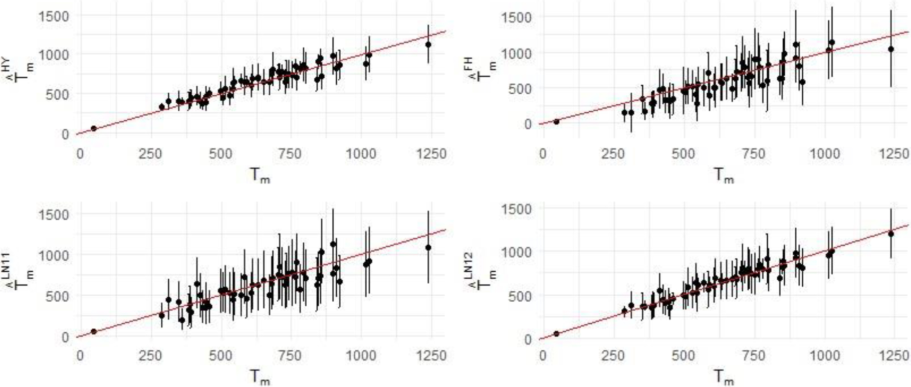
Plot of $\hat{T}_{m},\hat{T}_{m}^{\textit{FH}}$ and their 95% error bars against $T_{m}$ . Notes: (1) Data are sourced from Table 1 (left plot) and [19] (right plot). Error band is defined as $\hat{T}_{m}^{I}\pm 1.96\sqrt{M\hat{S}E(\hat{T}_{m}^{I}})$ where $I=\textit{HY}$ or FH. (2) $T_{m}$ denotes the actual size of the small area $m$ , the superscript^HY represent hybrid estimate.

As observed in Fig. 1, [19] concluded from this analysis that CKNN estimates outperform FH estimates. Specifically, the CKNN estimates exhibit better accuracy (closeness to the red line) and reduced uncertainty (shorter vertical lines) compared to their FH counterparts.

4. Levelling the playing field

The juxtaposition of CKNN estimates with FH estimates, as illustrated in Fig. 1, presents an inequitable comparison for two key reasons. Firstly, CKNN estimates are derived from unit-level covariates, while FH estimates are based on area-level covariates. This inherent difference in the granularity of covariate information disadvantages the FH estimates in the performance comparison.

Secondly, the CKNN estimates employ a hybrid approach by integrating big data, survey data and predicted missing data (due to the under-coverage of big data) to generate SAEs. In contrast, whilst they can be hybridized as shown by the hybridized LN estimates below, FH estimates do not currently adopt a hybrid estimation strategy, relying solely on the survey data without taking advantage of the information available from big data.

Given that, at the unit level, volunteer status is a binary variable, the application of the BHF model, designed for continuous variables, is not suitable. In their book, [14] delineate an Empirical Best Linear Unbiased Prediction (EBLUP) approach (Section 9.5.2) and a Hierarchical Bayes (HB) approach (Section 10.13.2) specifically tailored for binary variables. The EBLUP approach is also extensively discussed in [26]. However, for the purposes of this paper, we opted for the LN model under the HB approach, because it can be considered the Bayesian equivalent of the BHF model, it is applicable for binary response variables and software exists to facilitate with number crunching for HB models.

From a computational standpoint, the preference for the Hierarchical Bayes (HB) approach is substantiated by the availability of version 0.7.7 the R package, mcmcsae in the Comprehensive R Archive Network. Developed by Dr. HJ Boonstra of the Central Bureau of Statistics in the Netherlands. This package provides pre-built MCMC methods. These methods facilitate the generation of samples from the posterior distribution of SAE estimates, accommodating both continuous and binary target variables. With mcmcsae, users can efficiently compute posterior mean (and quantile) estimates along with their credible intervals, thus simplifying one’s computational burden.

For the 1% 2016 Census data, we use the LN model (equation 10.11.7 of [14]) for the volunteer data as follows:

(i)
$y_{m_{i}}|p_{m_{i}}\sim\textit{ind}$ Bernoulli ( $p_{m_{i}})$
(ii)
Logit ( $p_{m_{i}})=x_{m_{i}}^{T}\beta+\nu_{m}$ with $\nu_{m}\sim\textit{indN}$ $(0,\sigma_{\upsilon}^{2})$
(iii)
$\beta$ and $\sigma_{\upsilon}^{2}$ are mutually independent with $f(\beta)\propto 1$ and $\sigma_{\upsilon}^{-2}\sim G(a,b),a\geqslant 0,b>0,$ where $G(a,b)$ denotes the Gamma distribution with parameters $a$ and $b$ .

Utilising mcmcsae, Gibbs sampling was applied to the posterior distribution of $\psi=\{\beta,\nu_{1},\ldots,\nu_{M},\sigma_{\upsilon}^{2}\}$ to generate 2,000 non-burned-in MCMC samples of $\psi,$ with the Gelman-Rubin’s R_hat of each of $\psi$ lying between 0.9999 and 1.0017 demonstrating convergence. These are then plugged into (ii) to compute 2,000 estimates of $p_{m_{i}}$ , from which the posterior mean and credible intervals of $p_{m_{i}}$ are computed. For further details, refer to [14].

Using the LN model, we generated two sets of LN estimates for the small areas, denoted as $\hat{T}_{m}^{\textit{LN1}}$ and $\hat{T}_{m}^{\textit{LN2}}$ respectively, along with their credible intervals by $\hat{S}D^{\textit{LN1}}$ and $\hat{S}D^{\textit{LN2}}$ respectively. The $\hat{T}_{m}^{\textit{LN1}}$ is compiled without incorporating the big data in the estimation process, while $\hat{T}_{m}^{\textit{LN2}}$ employs a hybrid estimation approach akin to the method employed in CKNN estimates with the exception that calibration to the independent national total which is based on pro-rata, as the LN estimates is only 0.2% higher than the independent national benchmark total. These estimates were tabulated in the last four columns in Table 1, and visually represented in Fig. 2. The diagram on the left of the lower panel in Fig. 2 plots the LN1 data, and the diagram on the right plots the LN2 data.

From Table 1, we make the following observations:

Figure 2.
Plot of $\hat{T}_{m}^{HY},\hat{T}_{m}^{FH}$ , $\hat{T}_{m}^{LN1},\hat{T}_{m}^{LN2}$ and their 95% error bars against $T_{m}$ . a. Notes: (1) Data are sourced from Table 1 (upper left, lower left and left right plots) and [19] (upper right). Error band is defined as $\hat{T}_{m}^{I}\pm 1.96\psi$ where $\psi$ denotes root MSE (upper panel) and credible interval (lower panel). (2) $T_{m}$ denotes the actual size of the small area $m$ , the superscripts ^{HY, FH, LN1 and LN2} represent hybrid, Fay-Herriot,logit-normal and hybridized logit-normal estimates respectively.

1.
Without calibration, the national sum of the small area estimates from both LN estimates are further away (i.e. less accurate) from the actual number of volunteers of 35,742 than that of the CKNN estimates.
2.
The average absolute estimation error of CKNN estimates is smaller (i.e. more accurate) than the LN1 estimates, but higher (i.e. less accurate) than the LN2 estimates, suggesting the LN2 estimates are slightly more on target than CKNN estimates – an error of 42 for the LN2 estimates as compared with 57 for the CKNN estimates.
3.
The average relative root mean square error of the CKNN estimates is the smallest (i.e. the most accurate) and is 11% compared with 15% for LN2 estimates.
4.
The coverage rate of LN1 and LN2 estimates are numerically (but not statistically) higher than the CKNN estimates.

From Fig. 2, the following observations can be made:

1.
The CKNN (i.e. the hybrid estimates) plot (diagram on the left on the top panel) is better than the LN1 plot (diagram on left of the bottom panel), both in terms of numerical accuracy of the prediction, and reduction in uncertainty.
2.
The CKNN plot is worse than the LN2 plot (diagram on right of the bottom panel) in terms of numerical accuracy but better in terms of reduction in uncertainty.
3.
The performance of LN1 estimates is comparable with that of the FH estimates. At first glance, this contrasts with findings in the literature [15, 16]. However, those studies assume the linking model – specifically, assumption (ii) of the LN model – perfectly explains the target variable. The 2016 Census data, however, does not substantiate this assumption.
4.
Comparing the LN1 with the LN2 plots, it is evident that hybrid estimation is superior to no hybrid estimation.

5. Conclusion

The key results outlined in this paper underscore the superiority of CKNN estimates over LN and FH estimates, albeit with a notable reduction in this superiority when juxtaposed with hybridised LN estimation. Regardless of what methods one may choose for SAE, this result underpins the importance of adopting hybrid estimation.

It should be noted that the methods outlined in this paper require certain assumptions to be fulfilled [19]. They are:

The target variables, which are also collected in the survey, $A,$ are observed throughout the big data set without measurement errors – this condition is more likely to be satisfied when using administrative data for hybrid estimation than using many other types of big data. Where this condition is not satisfied, $A\cap B$ can be used as a training data set to construct a measurement error model to adjust the target variables in big data [28];

there are no over-coverage errors in the big data. Where this is not the case, $A_{m}\cap B_{m}$ can be used to estimate over-coverage rates in the small areas to remove the bias from $T_{B_{m}}$ ;

the donor set, $D,$ which depends on the size of $B$ and $A$ has to be sufficiently large, to support the imputations;

$\delta_{m}$ is fully observed for the units in the survey data set, $A$ – this can generally be made possible by matching the units between $A$ and $B$ through direct matching or probability matching [29]. When $\delta_{m}$ is not observed, or observed with error, one may use a semi-supervised classification technique to compute an EM estimator for $\delta_{m}$ [21]; and

associated with each unit of the population, there is a set of covariates which are available and known to the statistician. The assumption presumes the existence of a database with covariates covering the whole of the population.

The drawback of nearest neighbour methods arises when the dimensionality, i.e. $p,$ becomes too large [27, p. 22]. In such cases, the methods are susceptible to the curse of dimensionality, wherein the donors are positioned so far apart that they no longer genuinely qualify as nearest neighbours. In our numerical example, with $p=$ 3, the CKNN estimates of the total number of volunteers in small areas are not affected by this phenomenon.

An attraction of the CKNN method is in the variable-agnostic nature of the KNN algorithm. Put differently, this singular algorithm, configured only once, can be seamlessly applied to a spectrum of target variables. In contrast to the LN method, there is no necessity to construct variable-specific linking models for each target variable. This attribute allows the NSO to swiftly generate SAEs across a wide array of target variables. Additionally, in scenarios where unit record files are generated by the NSO for subsequent secondary analysis by researchers, the imputed data over this diverse array of target variables exhibit internal consistency across them without the need for further statistical processing.

Footnotes

Acknowledgments

We would like to thank Dr HJ Boonstra for his helpful advice on using mcmcsae to run the logit-normal model, and the two referees for their helpful comments on an earlier version of this paper.

Disclaimer

Views expressed in this paper are those of the author and do not necessarily represent those of the Australian Bureau of Statistics.

References

Fay

Herriot

. Estimates of Income for Small Places – An Application of James-Stein Procedures to Census data. Journal of the American Statistical Association. 1979; 74: 269-277.

Battese

Harter

Fuller

. An Error Component Model for Prediction of County Crop Areas Using Survey and Satellite Data. Journal of the American Statistical Association. 1988; 83: 28-36.

Pfeffermann

. Tiller

. Small area estimation with state-space models subject to benchmark constraints. Journal of the American Statistical Association. 2006; 101: 1387-1397.

Lehtone

Veijanen

. Design-based methods of estimation for domains and small areas. In Pfeffermann

Rao

. editors. Sample Surveys: Inference and Analysis Handbook of Statistics. Amsterdam: North-Holland; 2009; pp. 219–249.

Datta

. Model-based approach to small area estimation. In Pfeffermann

Rao

. editors. Sample Surveys: Inference and Analysis. Handbook of Statistics. Amsterdam: North-Holland. 2009; pp. 251-288.

Ghosh

Rao

JNK

. Small area estimation: An appraisal. Statistical Science. 1994; 9: 55-93.

Ghosh

. Small area estimation: its evolution in five decades. Statistics in Transition New Series; 21: 1-22.

Jiang

Lahiri

. Estimation of finite population domain means – A model-assisted empirical best prediction approach. Journal of the American Statistical Association. 2006; 101: 301-311.

Jiang

Lahiri,

. Mixed model prediction and small area estimation. Test. 2006; 15: 1-96.

10.

Pfeffermann

. Small area estimation – New developments and directions. International Statistical Review. 2002; 70: 125-143.

11.

Pfeffermann

. New important developments in small area estimation. Statistical Science 2013; 28: 40-68.

12.

Rao

JNK

. Inferential issues in small area estimation: Some new developments. Statistics in Transition. 2005; 7: 513-526.

13.

Rao

JNK

. Some methods for small area estimation. Revista Internazionale di Siencze Sociali. 2008; 4: 387-406.

14.

Rao

JNK

Molina

. Small Area Estimation. New York: John Wiley & Sons; 2015.

15.

Fay

. Further comparison of unit – and area – level small area estimators. Proceeding of the Survey Research Methods Section. 2018; 2057-2070.

16.

Hidiroglou

You

. Comparison of Unit Level and Area Level Small Area Estimators. Survey Methodology. 2016; 42: 41-61.

17.

Daas

PJH

Puts

van den Hurk

PAM

. Big data as a source for official statistics. Journal of Official Statistics 2015; 31: 249-262.

18.

Tam

Clarke

. Big data, official statistics and some initiative by the Australian Bureau of Statistics. International Statistical Review. 2015; 83: 436-448.

19.

Tam

Sharmeen

. A Calibrated Data-Driven Approach for Small Area Estimation using Big Data. Australian and New Zealand Journal of Statistics. 2024; 66: 125-145.

20.

Tam

Kim

Ang

Pham

. Mining the new oil for official statistics. In Hill

Biemer

Buskirk

Japec

Kitchner

Kolenikov

Lyberg

, editors. Big Data Meets Survey Science: A Collection of Innovation Methods. New York: John Wiley and Sons; 2020.

21.

Kim

Tam

. Data integration by combining big data and survey sample data for finite population inference. International Statistical Review. 2021; 89: 382-401.

22.

Hassanat

. Dimensionality Invariant Similarity Measure. Journal of American Science. 2014; 10: 221-226.

23.

Deville

Särndal

. Calibration estimators in survey sampling. Journal of the American Statistical Association. 1992; 87: 376-382.

24.

Otsu

Rai

. Bootstrap inference of matching estimators for average treatment effects. Journal of the American Statistical Association. 2017; 112: 1720-1732.

25.

Efron

. Better boostrap confidence intervals. Journal of the American Statistical Association. 1987; 82: 171-185.

26.

Hobza

Morale

. Empirical best prediction under unit-level logit mixed models. Journal of Official Statistics. 2016; 32: 661.

27.

Hastie

Tibshirani

Friedman

. The Elements of Statistical Learning: Data Mining, Inference and Prediction. New York: Springer; 2008.

28.

Medious

Goga

Ruiz-Gazen

Beaumont

Dessertaine

. Puech

. QR prediction for statistical data integration; 2023; [cited 2024 Aug 8]. Available from: https//www.tse-fr.eu/publications/qr-prediction-statistical-data-integration.

29.

Fellegi

Sunter

. A theory for record linkage. Journal of the American Statistical Association 1969; 40: 1183-1210.

Small data estimation for binary variables with big data: A comparison of calibrated nearest neighbour and hierarchical Bayes methods of estimation

Abstract

Keywords

1. Introduction

2. Harnessing big data for SAE

2.1 Notation and the underlying idea

2.2 The KNN algorithm

2.3 The CKNN algorithm

2.4 Estimating the MSE of T ^ m

3. Performance of the CKNN algorithm

Table 1 Estimates for T m , T ^ m 𝐻𝑌 , 𝑅𝑇𝑀 ⁢ S ^ ⁢ E 𝐻𝑌 ⁢ T ^ m LN1 , S ^ ⁢ D LN1 , T ^ m LN2 and S ^ ⁢ D LN2

Footnotes

Acknowledgments

Disclaimer

References

2.4 Estimating the MSE of $\hat{T}_{m}$

Table 1
Estimates for $T_{m}$ , $\hat{T}_{m}^{\textit{HY}}$ , $\textit{RTM}\hat{S}E^{\textit{HY}}\hat{T}_{m}^{\textit{LN1}}$ , $\hat{S}D^{\textit{LN1}}$ , $\hat{T}_{m}^{\textit{LN2}}$ and $\hat{S}D^{\textit{LN2}}$