Semantics and canonicalisation of SPARQL 1.1

Abstract

We define a procedure for canonicalising SPARQL 1.1 queries. Specifically, given two input queries that return the same solutions modulo variable names over any RDF graph (which we call congruent queries), the canonicalisation procedure aims to rewrite both input queries to a syntactically canonical query that likewise returns the same results modulo variable renaming. The use-cases for such canonicalisation include caching, optimisation, redundancy elimination, question answering, and more besides. To begin, we formally define the semantics of the SPARQL 1.1 language, including features often overlooked in the literature. We then propose a canonicalisation procedure based on mapping a SPARQL query to an RDF graph, applying algebraic rewritings, removing redundancy, and then using canonical labelling techniques to produce a canonical form. Unfortunately a full canonicalisation procedure for SPARQL 1.1 queries would be undecidable. We rather propose a procedure that we prove to be sound and complete for a decidable fragment of monotone queries under both set and bag semantics, and that is sound but incomplete in the case of the full SPARQL 1.1 query language. Although the worst case of the procedure is super-exponential, our experiments show that it is efficient for real-world queries, and that such difficult cases are rare.

Keywords

SPARQL RDF query semantics caching canonicalisation congruence equivalence

1. Introduction

The Semantic Web provides a variety of standards and techniques for enhancing the machine-readability of Web content in order to increase the levels of automation possible for day-to-day tasks. RDF [54] is the standard framework for the graph-based representation of data on the Semantic Web. In turn, SPARQL [24] is the standard querying language for RDF, composed of basic graph patterns extended with expressive features that include path expressions, relational algebra, aggregation, federation, among others.

The adoption of RDF as a data model and SPARQL as a query language has grown significantly in recent years [4,26]. Prominent datasets such as DBpedia [35] and Wikidata [61] contain in the order of hundreds of millions or even billions of RDF triples, and their associated SPARQL endpoints receive millions of queries per day [37,52]. Hundreds of other SPARQL endpoints are likewise available on the Web [4]. However, a survey carried out by Buil-Aranda et al. [4] found that a large number of SPARQL endpoints experience performance issues such as latency and unavailability. The same study identified the complexity of SPARQL queries as one of the main causes of these problems, which is perhaps an expected result given the expressivity of the SPARQL query language where, for example, the decision problem consisting of determining if a solution is given by a query over a graph is $PS PACE - hard$ for the SPARQL language [44].

One way to address performance issues is through caching of sub-queries [41,62]. The caching of queries is done by evaluating a query, then storing its result set, which can then be used to answer future instances of the same query without using any additional resources. The caching of sub-queries identifies common query patterns whose results can be returned for queries that contain said query patterns. However, this is complicated by the fact that a given query can be expressed in different, semantically equivalent ways. As a result, if we are unable to verify if a given query is equivalent to one that has already been cached, we are not using the cached results optimally: we may miss relevant results.

Ideally, for the purposes of caching, we could use a procedure to canonicalise SPARQL queries. To formalise this idea better, we call two queries equivalent if (and only if) they return the same solutions over any RDF dataset. Note however that this notion of equivalence requires the variables of the solutions of both queries to coincide. In practice, variable names will often differ across queries, where we would still like to be able to cache and retrieve the results for queries whose results are the same modulo variable names. Hence we call two queries congruent if they return the same solutions, modulo variable names, over any RDF dataset; in other words, two queries are congruent if (and only if) there exists a one-to-one mapping from the variables in one query to the variables of the other query that makes the former equivalent to the latter.

In this paper, we propose a procedure by which congruent SPARQL queries can be “canonicalised”. We call such a procedure sound if the output query is congruent to the input query, and complete if the same output query is given for any two congruent input queries.

Example 1.1.
Consider the following two SPARQL queries asking for names of aunts: Both queries are equivalent: they always return the same results for any RDF dataset. Now rather consider a third SPARQL query: Note that the pattern ?b :name ?n . in this query is redundant. This query is not equivalent to the former two because the variable that is returned is different, and thus the solutions (which contain the projected variable), will not be the same. However all three queries are congruent; for example, if we rewrite ?n to ?z in the third query, all three queries become equivalent.

Canonicalisation aims to rewrite all three (original) queries to a unique, congruent, output query.

The potential use-cases we foresee for a canonicalisation procedure include the following:
Query caching:
As aforementioned, a canonicalisation procedure can improve caching for SPARQL endpoints. By capturing knowledge about query congruence, canonicalisation can increase the cache hit rate. Similar techniques could also be used to identify and cache frequently appearing (congruent) sub-queries [41].
Views:
In a conceptually similar use case to caching, our canonical procedure can be used to describe views [9]. In particular, the canonicalisation procedure can be used to create a key that uniquely identifies each of the views available.
Log analysis:
SPARQL endpoint logs can be analysed in order to understand the importance of different SPARQL features [7,52], to build suitable benchmarks [52], to understand how users build queries incrementally [7,64], etc. Our canonicalisation procedure could be used to pre-process and group congruent queries in logs.
Query optimisation:
Canonicalisation may help with query optimisation by reducing the variants to be considered for query planning, detecting duplicate sub-queries that can be evaluated once, removing redundant patterns (as may occur under query rewriting strategies for reasoning [33]), etc.
Learning over queries:
Canonicalisation can reduce superficial variance in queries used to train machine learning models. For example, recent question answering systems learn translations from natural language questions to queries [10], where canonicalisation can be used to homogenise the syntax of queries used for training.

Other possible but more speculative use-cases involve signing or hashing SPARQL queries, discovering near-duplicate or parameterised queries (by considering constants as variables), etc. Furthermore, with some adaptations, the methods proposed here could be generalised to other query languages, such as to canonicalise SQL queries, Cypher queries [3], etc.

A key challenge for canonicalising SPARQL queries is the prohibitively high computational complexity that it entails. More specifically, the query equivalence problem takes two queries and returns true if and only if they return the same solutions for any dataset, or false otherwise. In the case of SPARQL, this problem is intractable ( $NP- complete$ ) even when simply permitting joins (with equality conditions). Even worse, the problem becomes undecidable when features such as projection and optional matches are added [45]. Since a canonicalisation procedure can be directly used to decide equivalence, this means that canonicalisation is at least as hard as the equivalence problem in computational complexity terms, meaning it will likewise be intractable for even simple fragments and undecidable when considering the full SPARQL language. There are thus fundamental limitations in what can be achieved for canonicalising SPARQL queries.

With these limitations in mind, we propose a canonicalisation procedure that is always sound, but only complete for a monotone fragment of SPARQL under set or bag semantics. This monotone fragment permits unions and joins over basic graph patterns, some examples of which were illustrated in Example 1.1. We further provide sound, but incomplete, canonicalisation of the full SPARQL 1.1 query language, whereby the canonicalised query will be congruent to the input query, but not all pairs of congruent input queries will result in the same output query. In the case of incomplete canonicalisation, we are still able to find novel congruences, in particular through canonical labelling of variables, which further allows for ordering operands in a consistent manner. Reviewing the aforementioned use-cases, we believe that this “best-effort” form of canonicalisation is still useful, as in the case of caching, where missing an equivalence will require re-executing the query (which would have to be done in any case), or in the case of learning over queries, where incomplete canonicalisation can still increase the homogeneity of the training examples used.

As a high-level summary, our procedure combines four main techniques for canonicalisation.

The first technique is to convert SPARQL queries to an algebraic graph, which abstracts away syntactic variances, such as the ordering of operands for operators that are commutative, and the grouping of operands for operators that are associative.

The second technique is to apply algebraic rewritings on the graph to achieve normal forms over combinations of operators. For example, we rewrite monotone queries – that allow any combination of join, union, basic graphs patterns, etc. – into unions of basic graph patterns; this would rewrite the first and third queries shown in Example 1.1 into a form similar to the second query.

The third technique is to apply redundancy elimination within the algebraic graph, which typically involves the removal of elements of the query that do not affect the results; this technique would remove the redundant ?b :name ?n . pattern from the third query of Example 1.1.

The fourth and final technique is to apply a canonical labelling of the algebraic graph, which will provide consistent labels to variables, and which in turn allows for the (unordered) algebraic graph to be serialised back into the (ordered) concrete syntax of SPARQL in a canonical way.

We remark that the techniques do not necessarily follow the presented order; in particular, the second and third techniques can be interleaved in order to provide further canonicalisation of queries.

This paper extends upon our previous work [50] where we initially outlined a sound and complete procedure for canonicalising monotone SPARQL queries. The novel contributions of this extended paper include:

We close a gap involving translation of monotone queries under bag semantics that cannot return duplicates into set semantics.

We provide a detailed semantics for SPARQL 1.1 queries; formalising and understanding this is a key prerequisite for canonicalisation.

We extend our algebraic graph representation in order to be able to represent SPARQL 1.1 queries, offering partial canonicalisation support.

We implement algebraic rewriting rules for specific SPARQL 1.1 operators, such as those relating to filters; we further propose techniques to canonicalise property path expressions.

We provide more detailed experiments, which now include results over a Wikidata query log, a comparison with existing systems from the literature that perform pairwise equivalence checks, and more detailed stress testing.

We also provide extended proofs of results that were previously unpublished [51], as well as providing extended discussion and examples throughout.

The outline of the paper is then as follows. Section 2 provides preliminaries for RDF, while Section 3 provides a detailed semantics for SPARQL. Section 4 provides a problem statement, formalising the notion of canonicalisation. Section 5 discusses related works in the areas of systems that support query containment, equivalence, and congruence. Sections 6 and 7 discuss our SPARQL canonicalisation framework for monotone queries, and SPARQL 1.1, respectively. Section 8 presents evaluation results. Section 9 concludes.
2. RDF data model

We begin by introducing the core concepts of the RDF data model over which the SPARQL query language will later be defined. The following is a relatively standard treatment of RDF, as can be found in various papers from the literature [22,28]. We implicitly refer to RDF 1.1 unless otherwise stated.

2.1. Terms and triples

RDF assumes three pairwise disjoint sets of terms: IRIs (I), literals (L) and blank nodes (B). Data in RDF are structured as triples, which are 3-tuples of the form $(s, p, o) \in I B \times I \times I B L$ denoting the subject s, the predicate p, and the object o of the triple.1

¹
In this paper we concatenate set names to denote their union; e.g., $I B L$ is used as an abbreviation for the union $I \cup B \cup L$ .

There are three types of literals: a plain literal s is a simple string, a language-tagged literal

(s, l)

is a pair of a simple string and a language tag, and

(s, d)

is a pair of a simple string and an IRI (denoting a datatype).

In this paper we use Turtle/SPARQL-like syntax, where :a, xsd:string, etc., denote IRIs; _:b, _:x1, etc., denote blank nodes; "a", "xy z", etc., denote plain literals; "hello"@en, "hola"@es, etc., denote language-tagged literals; and "true" $^$ $^$ xsd:boolean, "1" $^$ $^$ xsd:int, etc., denote datatype literals.

2.2. Graph

An RDF graph G is a set of RDF triples. It is called a graph because each triple $(s, p, o) \in G$ can be viewed as a directed labelled edge of the form $s \overset{p}{\to} o$ , and a set of such triples forms a directed edge-labelled graph.

2.3. Simple entailment and equivalence

Blank nodes in RDF have special meaning; in particular, they are considered to be existential variables. The notion of simple entailment [22,25] captures the existential semantics of blank nodes (among other fundamental aspects of RDF). This same notion also plays a role in how the SPARQL query language is defined.

Formally, let $α : B \to I B L$ denote a mapping that maps blank nodes to RDF terms; we call such a mapping a blank node mapping. Given an RDF graph G, let $bnodes (G)$ denote all of the blank nodes appearing in G. Let $α (G)$ denote the image of G under α; i.e., the graph G but with each occurrence of each blank node $b \in bnodes (G)$ replaced with $α (b)$ . Given two RDF graphs G and H, we say that G simple-entails H, denoted $G ⊧ H$ , if and only if there exists a blank node mapping α such that $α (H) \subseteq G$ [22,25]. Furthermore, if $G ⊧ H$ and $H ⊧ G$ , then we say that they are simple equivalent, denoted $G \equiv H$ .

Deciding simple entailment $G ⊧ H$ is known to be $NP- complete$ [22]. Deciding the simple equivalence $G \equiv H$ is likewise known to be $NP- complete$ .

We remark that the RDF standard defines further entailment regimes that cover the semantics of datatypes and the special RDF and RDFS vocabularies [25]; we will not consider such entailment regimes here.

2.4. Isomorphism

Given that blank nodes are defined as existential variables [25], two RDF graphs differing only in blank node labels are thus considered isomorphic [19,28].

Formally, if a blank node mapping of the form $α : B \to B$ is one-to-one, we call it a blank node bijection. Two RDF graphs G and H are defined as isomorphic, denoted $G ≃ H$ , if and only if there exists a blank node bijection α such that $α (G) = H$ ; i.e., the two RDF graphs differ only in their blank node labels. We remark that if $G ≃ H$ , then $G \equiv H$ ; however, the inverse does not always hold as we discuss in the following.

Deciding the isomorphism $G ≃ H$ is known to be $GI- complete$ [28] (as hard as graph isomorphism).

2.5. Leanness and core

Existential blank nodes may give rise to redundant triples. In particular, an RDF graph G is called lean if and only if there does not exist a proper subgraph $G^{'} ⊊ G$ of it such that $G^{'} ⊧ G$ ; otherwise G is called non-lean. Non-lean graphs can be seen, under the RDF semantics, as containing redundant triples. For example, given an RDF graph $G = {(:x, :y, :z), (:x, :y,_:b)}$ , the second triple is seen as redundant: it states that :x has some value on :y, but we know this already from the first triple, so the second triple says nothing new.

The core of an RDF graph G is then an RDF graph $G^{'}$ such that $G^{'} \equiv G$ and $G^{'}$ is lean; intuitively it is a version of G without redundancy. For example the core of the aforementioned graph would be $G^{'} = {(:x, :y, :z)}$ ; note that $G^{'} \equiv G$ and $G^{'}$ is lean, but $G^{'} ≄ G$ . The core of a graph is unique modulo isomorphism [22]; hence we refer to the core of a graph.

Deciding whether or not an RDF G is lean is known to be $CO NP- complete$ [22]. Deciding if $G^{'}$ is the core of G is known to be $DP- complete$ [22].

2.6. Merge

Blank nodes are considered to be scoped to a local RDF graph. Hence when combining RDF graphs, applying a merge (rather than union) avoids blank nodes with the same name in two (or more) graphs clashing. Given two RDF graphs G and $G^{'}$ , and a blank node bijection α such that $bnodes (α (G)) \cap bnodes (G^{'}) = \emptyset$ , we call $α (G) \cup G^{'}$ an RDF merge, denoted $G ⊎ G^{'}$ . The merge of two graphs is unique modulo isomorphism.

3. SPARQL 1.1 semantics

We now define SPARQL 1.1 in detail [24]. We will begin by defining a SPARQL dataset over which queries are evaluated. We then introduce an abstract syntax for SPARQL queries. Thereafter we discuss the evaluation of queries under different semantics.

These definitions extend similar preliminaries found in the literature. However, our definitions of the semantics of SPARQL 1.1 extend beyond the core of the language and rather aim to be exhaustive, where a clear treatment of the full language is a prerequisite for formalising the canonicalisation of queries using the language. Table 1 provides a summary of prior works that have defined the semantics of SPARQL features. We exclude works that came after one of the works shown and use a subset of the features of that work (even if they may contribute novel results about those features). Some SPARQL 1.0 features, such as UNION, FILTER and OPTIONAL, have been featured in all studies. In terms of SPARQL 1.1, the most extensive formal definitions have been provided by Polleres and Wallner [47], and by Kaminski et al. [32]. However, both works omit query features: Polleres and Wallner [47] omit federation and aggregation, whereas Kaminski et al. [32] omit named graphs, federation, and non-SELECT query forms. Compared to these previous works, we aim to capture the full SPARQL 1.1 query language, with one simplification: we define functions and expressions abstractly, rather than defining all of the many built-ins that SPARQL 1.1 provides (e.g., +, BOUND, COUNT, IF, etc.)

Table 1
Studies that define the semantics of features in SPARQL (1.1), including Monotone (basic graph patterns, joins, UNION, un-nested SELECT DISTINCT), Filters, Optionals, Negation (OPTIONAL & !BOUND, MINUS, FILTER (NOT) EXISTS), Named Graphs (GRAPH, FROM (NAMED)), Paths, Federation (SERVICE), Assignment (BIND, VALUES), Aggregation (GROUP BY and aggregate functions), Sub Queries (nested SELECT), Solution Modifiers (LIMIT, OFFSET, ORDER BY), Query Forms (CONSTRUCT, ASK, DESCRIBE), Expressions and Functions (e.g., +, BOUND, COUNT, IF), Bag Semantics; we denote by “” partial definitions or discussion

Paper Year Mon Filt Opt Neg NGra Path Fed Assn Agg SubQ SolM Form Exp Bag

Perez et al. [43,44] 2006 ✓ ✓ ✓ *

Polleres [46] 2007 ✓ ✓ ✓ * ✓ * * *

Alkhateeb et al. [2] 2009 ✓ ✓ ✓ * ✓ *

Arenas and Pérez [5] 2012 ✓ ✓ ✓ * * ✓ ✓ * * ✓

Polleres and Wallner [47] 2013 ✓ ✓ ✓ ✓ ✓ ✓ ✓ ✓ ✓ * * ✓

Kaminski et al. [32] 2017 ✓ ✓ ✓ ✓ ✓ ✓ ✓ ✓ * * ✓

Salas and Hogan 2021 ✓ ✓ ✓ ✓ ✓ ✓ ✓ ✓ ✓ ✓ ✓ ✓ * ✓

Paper	Year	Mon	Filt	Opt	Neg	NGra	Path	Fed	Assn	Agg	SubQ	SolM	Form	Exp	Bag
Perez et al. [43,44]	2006	✓	✓	✓	*									*
Polleres [46]	2007	✓	✓	✓	*	✓					*		*	*
Alkhateeb et al. [2]	2009	✓	✓	✓	*		✓							*
Arenas and Pérez [5]	2012	✓	✓	✓	*	*	✓	✓	*					*	✓
Polleres and Wallner [47]	2013	✓	✓	✓	✓	✓	✓		✓		✓	✓	*	*	✓
Kaminski et al. [32]	2017	✓	✓	✓	✓		✓		✓	✓	✓	*		*	✓
Salas and Hogan	2021	✓	✓	✓	✓	✓	✓	✓	✓	✓	✓	✓	✓	*	✓

Table 2

SPARQL property path syntax

The following are path expressions
p	a predicate (IRI)
$!(p_{1} \| \dots \| p_{k} \|^p_{k + 1} \| \dots \|^p_{n})$	any (inv.) predicate not listed
and if e , $e_{1}$ , $e_{2}$ are path expressions the following are also path expressions:
$^e$	an inverse path
$e_{1} / e_{2}$	a path of $e_{1}$ followed by $e_{2}$
$e_{1} \| e_{2}$	a path of $e_{1}$ or $e_{2}$
$e *$	a path of zero or more e
$e +$	a path of one or more e
$e ?$	a path of zero or one e
(e)	brackets used for grouping

3.1. Query syntax

Before we introduce an abstract syntax for SPARQL queries, we provide some preliminaries:

A triple pattern $(s, p, o)$ is a member of the set $V I B L \times V I \times V I B L$ (i.e., an RDF triple allowing variables in any position and literals as subject).

A basic graph pattern B is a set of triple patterns. We denote by $vars B : = ⋃_{(s, p, o) \in B} V \cap {s, p, o}$ the set of variables used in B.

A path pattern $(s, e, o)$ is a member of the set $V I B L \times P \times V I B L$ , where P is the set of all path expressions defined by Table 2.

A navigational graph pattern N is a set of paths patterns and triple patterns (with variable predicates). We denote by $vars N : = ⋃_{(s, e, o) \in N} V \cap {s, e, o}$ the set of variables used in N.

A term in $V I B L$ is a built-in expression. Let ⊥ denote an unbound value and ε an error. We call ϕ a built-in function if it takes a tuple of values from $I B L \cup {⊥, ε}$ as input and returns a single value in $I B L \cup {⊥, ε}$ as output. An expression $ϕ (R_{1}, \dots, R_{n})$ , where each $R_{1}, \dots, R_{n}$ is a built-in expression, is itself a built-in expression.

An aggregation function ψ is a function that takes a bag of tuples from $I B L$ as input and returns a value in $I B L \cup {⊥, ε}$ as output. An expression $ψ (R_{1}, \dots, R_{n})$ , where each $R_{1}, \dots, R_{n}$ is a built-in expression, is an aggregation expression.

If R is a built-in expression, and Δ is a boolean value indicating ascending or descending order, then $(R, Δ)$ is an order comparator.

We then define the abstract syntax of a SPARQL query as shown in Table 3. Note that we abbreviate OPTIONAL as opt, FILTER EXISTS as fe, and FILTER NOT EXISTS as fne. Otherwise mapping from SPARQL’s concrete syntax to this abstract syntax is straightforward, with the following exceptions:

For brevity, we consider the following SPARQL 1.1 operators to be represented as functions:

boolean operators: ! for negation, && for conjunction, || for disjunction;

equality and inequality operators: =, <, >, <=, >=, !=;

numeric operators: unary + and - for positive/negative numbers; binary + and - for addition/subtraction, * for multiplication and / for division;

for example, replacing

?a + ?b

, we assume addition to be defined as a function

SUM (?a, ?b)

We combine FROM and FROM NAMED into one feature, from, so they can be evaluated together.

A query such as DESCRIBE <x> <y> in the concrete syntax can be expressed in the abstract syntax with an empty pattern ${DESCRIBE}_{{x, y}} ({})$ .

Aggregates without grouping can be expressed with ${GROUP}_{{}} (Q) (D)$ . We assume that every query in the abstract syntax with a group-by pattern uses agg – possibly ${AGG}_{{}} (Q)$ – to generate a graph pattern (and “flatten” groups).

Some aggregation functions in SPARQL take additional arguments, including a DISTINCT modifier, or a delimiter in the case of CONCAT. For simplicity, we assume that these are distinct functions, e.g., count(·) versus countdistinct(·).

SPARQL allows SELECT * to indicate that values for all variables should be returned. Otherwise SPARQL requires that at least one variable be specified. A SELECT * clause can be written in the abstract syntax as ${SELECT}_{V} (Q)$ where Q is a graph pattern on V. Also the abstract syntax allows empty projections ${SELECT}_{{}} (Q)$ , which greatly simplifies certain definitions and proofs; this can be represented in the concrete syntax as SELECT ?empty, where ?empty is a fresh variable not appearing in the query.

In the concrete syntax, SELECT allows for built-in expressions and aggregation expressions to be specified. We only allow variables to be used. However, such expressions can be bound to variables using bind or agg.2

²
In our proposed abstract syntax and the concrete syntax, the ordering of variables in the SELECT is not meaningful, though in practice engines may often present variables in the results following the same order in which they are listed by the SELECT clause.

In the concrete syntax, ORDER BY allows for using aggregation expressions in the order comparators. Our abstract syntax does not allow this as it complicates the definitions of such comparators. Ordering on aggregation expressions can rather be achieved using sub-queries.

We use $[Q_{1} {SERVICE}_{x}^{Δ} Q_{2}]$ to denote SERVICE, where $Δ = true$ indicates the SILENT keyword is invoked, and $Δ = false$ indicates that it is not.

We do not consider SERVICE with variables as it has no normative semantics in the standard [48].

Aside from the latter point, these exceptions are syntactic conveniences that help simplify later definitions.

Table 3

Abstract SPARQL syntax

– B is a basic graph pattern.	∴ B is a graph pattern on $vars B$ .
– N is a navigational graph pattern.	∴ N is a graph pattern on $vars N$ .
– $Q_{1}$ is a graph pattern on $V_{1}$ .– $Q_{2}$ is a graph pattern on $V_{2}$ .	∴ [ $Q_{1} AND Q_{2}$ ] is a graph pattern on $V_{1} \cup V_{2}$ ;∴ [ $Q_{1} UNION Q_{2}$ ] is a graph pattern on $V_{1} \cup V_{2}$ ;∴ [ $Q_{1} OPT Q_{2}$ ] is a graph pattern on $V_{1} \cup V_{2}$ ;∴ [ $Q_{1} MINUS Q_{2}$ ] is a graph pattern on $V_{1}$ .
– Q is a graph pattern on V.– $Q_{1}$ is a graph pattern on $V_{1}$ .– $Q_{2}$ is a graph pattern on $V_{2}$ .– v is a variable not in V.– R is a built-in expression.	∴ ${FILTER}_{R} (Q)$ is a graph pattern on V;∴ $[Q_{1} FE Q_{2}]$ is a graph pattern on $V_{1}$ ;∴ $[Q_{1} FNE Q_{2}]$ is a graph pattern on $V_{1}$ ;∴ ${BIND}_{R, v} (Q)$ is a graph pattern on $V \cup {v}$ .
– Q is a graph pattern on V.– $M$ is a bag of solution mappings on $V_{M} = ⋃_{μ \in M} dom (μ)$ .	∴ ${VALUES}_{M} (Q)$ is a graph pattern on $V \cup V_{M}$ .
– Q is a graph pattern on V.– x is an IRI.– v is a variable.	∴ ${GRAPH}_{x} (Q)$ is a graph pattern on V.∴ ${GRAPH}_{v} (Q)$ is a graph pattern on $V \cup {v}$ .
– $Q_{1}$ is a graph pattern on $V_{1}$ .– $Q_{2}$ is a graph pattern on $V_{2}$ .– x is an IRI.– Δ is a boolean value.	∴ $[Q_{1} {SERVICE}_{x}^{Δ} Q_{2}]$ is a graph pattern on $V_{1} \cup V_{2}$ .
– Q is a graph pattern on V.– $Q^{'}$ is a group-by pattern on $(V^{'}, V)$ .– $V^{″}$ is a set of variables. – A is an aggregation expression– Λ is a (possibly empty) set of pairs ${(A_{1}, v_{1}), \dots, (A_{n}, v_{n})}$ , where $A_{1}$ , …, $A_{n}$ are aggregation expressions, $v_{1}$ , …, $v_{n}$ are variables not appearing in $V \cup V^{'}$ such that $v_{i} \neq v_{j}$ for $1 ⩽ i < j ⩽ n$ , and where $vars Λ = {v_{1}, \dots, v_{n}}$	∴ Q is a group-by pattern on (∅, V).∴ $Q^{'}$ is a graph pattern on $V^{'}$ .∴ ${GROUP}_{V^{″}} (Q)$ is a group-by pattern on $(V^{″}, V)$ .∴ ${HAVING}_{A} (Q^{'})$ is a group-by pattern on $(V^{'}, V)$ .∴ ${AGG}_{Λ} (Q^{'})$ is a graph pattern on $(V^{'} \cup vars Λ, V)$ .
– Q is a graph pattern or sequence pattern on V.– Ω is a non-empty sequence of order comparators.– k is a non-zero natural number.	∴ Q is a graph pattern and sequence pattern on V∴ ${ORDER}_{Ω} (Q)$ is a sequence pattern on V.∴ $DISTINCT (Q)$ is a sequence pattern on V.∴ $REDUCED (Q)$ is a sequence pattern on V.∴ ${OFFSET}_{k} (Q)$ is a sequence pattern on V.∴ ${LIMIT}_{k} (Q)$ is a sequence pattern on V.
– Q is a sequence pattern on V that does not contain the same blank node b in two different graph patterns.– $V^{'}$ is a set of variables.– B is a basic graph pattern.– X is a set of IRIs and/or variables.	∴ ${SELECT}_{V^{'}} (Q)$ is a query and a graph pattern on $V^{'}$ .∴ $ASK (Q)$ is a query.∴ ${CONSTRUCT}_{B} (Q)$ is a query.∴ ${DESCRIBE}_{X} (Q)$ is a query.
– Q is a query but not a from query– X and $X^{'}$ are sets of IRIs	∴ ${FROM}_{X, X^{'}} (Q)$ is a from query and a query.

3.2. Datasets

SPARQL allows for indexing and querying more than one RDF graph, which is enabled through the notion of a SPARQL dataset. Formally, a SPARQL dataset $D : = (G, {(x_{1}, G_{1}), \dots, (x_{n}, G_{n})})$ is a pair of an RDF graph G called the default graph, and a set of named graphs of the form $(x_{i}, G_{i})$ , where $x_{i}$ is an IRI (called a graph name) and $G_{i}$ is an RDF graph; additionally, graph names must be unique, i.e., $x_{j} \neq x_{k}$ for $1 ⩽ j < k ⩽ n$ . We denote by $G_{D}$ the default graph G of D and by $D^{*} = {(x_{1}, G_{1}), \dots, (x_{n}, G_{n})}$ the set of all named graphs in D. We further denote by $G_{D [x_{i}]}$ the graph $G_{i}$ such that $(x_{i}, G_{i}) \in D^{*}$ or the empty graph if $x_{i}$ does not appear as a graph name in $D^{*}$ .

3.3. Services

While the SPARQL standard defines a wide range of features that compliant services must implement, a number of decisions are left to a particular service. First and foremost, a service chooses what dataset to index. Along these lines, we define a SPARQL service as a tuple $S = (D, R, A, ⩽, describe)$ , where:

D is a dataset;

$R$ is a set of supported built-in expressions;

$A$ is a set of supported aggregation expressions;

⩽ is a total ordering of RDF terms and ⊥;

$describe$ is a function used to describe RDF terms.

We will denote by $D_{S}$ the dataset of a particular service. The latter two elements will be described in more detail as they are used. The SPARQL standard does define some minimal requirements on the set of built-in expressions, the set of aggregation expressions, the ordering of terms, etc., that a standards-compliant service should respect. We refer to the SPARQL standard for details on these requirements [24].

3.4. Query evaluation

The semantics of a SPARQL query Q can be defined in terms of its evaluation over a SPARQL dataset D, denoted $Q (D)$ which returns solution mappings that represent “matches” for Q in D.

3.4.1. Solution mappings

A solution mapping μ is a partial mapping from variables in V to terms $I B L$ . We denote the set of all solution mappings by M. Let $dom (μ)$ denote the domain of μ, i.e., the set of variables for which μ is defined. Given ${v_{1}, \dots, v_{n}} \subseteq V$ and ${x_{1} \dots, x_{n}} \subseteq I B L \cup {⊥}$ , we denote by ${v_{1} / x_{1}, \dots, v_{n} / x_{n}}$ the mapping μ such that $dom (μ) = {v_{i} ∣ x_{i} \notin {⊥, ε}}$ for $1 ⩽ i ⩽ n$ and $μ (v_{i}) = x_{i}$ for $v_{i} \in dom (μ)$ . We denote by $μ_{\emptyset}$ the empty solution mapping (such that $dom (μ_{\emptyset}) = \emptyset$ ).

We say that two solution mappings $μ_{1}$ and $μ_{2}$ are compatible, denoted $μ_{1} \sim μ_{2}$ , if and only if $μ_{1} (v) = μ_{2} (v)$ for every $v \in dom (μ_{1}) \cap dom (μ_{2})$ . We say that two solution mappings $μ_{1}$ and $μ_{2}$ are overlapping, denoted $μ_{1} * μ_{2}$ , if and only if $dom (μ_{1}) \cap dom (μ_{2}) \neq \emptyset$ .

Given two compatible solution mappings $μ_{1} \sim μ_{2}$ , we denote by $μ_{1} \cup μ_{2}$ their combination such that $dom (μ_{1} \cup μ_{2}) = dom (μ_{1}) \cup dom (μ_{2})$ , and if $v \in dom (μ_{1})$ then $(μ_{1} \cup μ_{2}) (v) = μ_{1} (v)$ , otherwise if $v \in dom (μ_{2})$ then $(μ_{1} \cup μ_{2}) (v) = μ_{2} (v)$ . Since the solution mappings $μ_{1}$ and $μ_{2}$ are compatible, for all $v \in dom (μ_{1}) \cap dom (μ_{2})$ , it holds that $(μ_{1} \cup μ_{2}) (v) = μ_{1} (v) = μ_{2} (v)$ , and thus $μ_{1} \cup μ_{2}$ = $μ_{2} \cup μ_{1}$ .

Given a solution mapping μ and a triple pattern t, we denote by $μ (t)$ the image of t under μ, i.e., the result of replacing every occurrence of a variable v in t by $μ (v)$ (generating an unbound ⊥ if $v \notin dom (μ)$ ). Given a basic graph pattern B, we denote by $μ (B)$ the image of B under μ, i.e., $μ (B) : = {μ (t) ∣ t \in B}$ . Likewise, given a navigational graph pattern N, we analogously denote by $μ (N)$ the image of N under μ.

Blank nodes in SPARQL queries can likewise play a similar role to variables though they cannot form part of the solution mappings. Given a blank node mapping α, we denote by $α (B)$ the image of B under α and by $bnodes (B)$ the set of blank nodes used in B; we define $α (N)$ and $bnodes (N)$ analogously.

Finally, we denote by $R (μ)$ the result of evaluating the image of the built-in expression R under μ, i.e., the results of replacing all variables v in R (including in nested expressions) with $μ (v)$ and evaluating the resulting expression. We denote by $μ ⊧ R$ that μ satisfies R, i.e., that $R (μ)$ returns a value interpreted as true.

3.4.2. Set vs. bag vs. sequence semantics

SPARQL queries can be evaluated under different semantics, which may return a set of solution mappings M, a bag of solution mappings $M$ , or a sequence of solution mappings $M$ . Sets are unordered and do not permit duplicates. Bags are unordered and permit duplicates. Sequences are ordered and permit duplicates.

Given a solution mapping μ and a bag of solution mappings $M$ , we denote by $M (μ)$ the multiplicity of μ in $M$ , i.e., the number of times that μ appears in $M$ ; we say that $μ \in M$ if and only if $M (μ) > 0$ (otherwise, if $M (μ) = 0$ , we say that $μ \notin M$ ). We denote by $| M | = \sum_{μ \in M} M (μ)$ the (bag) cardinality of $M$ . Given two bags $M$ and $M^{'}$ , we say that $M \subseteq M^{'}$ if and only if $M (μ) ⩽ M^{'} (μ)$ for all $μ \in M$ . Note that $M \subseteq M^{'}$ and $M^{'} \subseteq M$ if and only if $M = M^{'}$ .

Given a sequence $M$ of length n (we denote that $| M | = n$ ), we use $M [i]$ (for $1 ⩽ i ⩽ n$ ) to denote the i^th solution mapping of $M$ , and we say that $μ \in M$ if and only if there exists $1 ⩽ i ⩽ n$ such that $M [i] = μ$ . We denote by $M [i \dots j]$ (for $1 ⩽ i ⩽ j$ ) the sub-sequence $(M [i], M [i + 1], \dots, M [j - 1], M [j])$ of elements i to j of $M$ , inclusive, in order; if $i = j$ , then $M [i \dots j]$ is defined to be $(M [i])$ ; if $i > n$ , then $M [i \dots j]$ is defined to be the empty sequence $()$ ; otherwise if $j > n$ , then $M [i \dots j]$ is defined to be $M [i \dots n]$ . Given two sequences $M_{1}$ and $M_{2}$ , we denote by $M_{1} M_{2}$ their concatenation. For a sequence $M$ of length $n > 0$ , we define the deletion of index $i ⩽ n$ , denoted $del (M, i)$ , as the concatenation $M [1 \dots i - 1] M [i + 1 \dots n]$ if $1 < i ⩽ n$ , or $M [2 \dots n]$ if $i = 1$ , or $M [1 \dots n - 1]$ otherwise. We call j a repeated index of $M$ if there exists $1 ⩽ i < j$ such that $M [i] = M [j]$ . We define $dist (M)$ to be the fixpoint of recursively deleting repeated indexes from $M$ . We say that $M^{'}$ is contained in $M$ , denoted $M^{'} \subseteq M$ , if and only if we can derive $M^{'}$ by recursively removing zero-or-more indexes from $M$ . Note that $M^{'} \subseteq M$ and $M \subseteq M^{'}$ if and only if $M = M^{'}$ .

Next we provide some convenient notation to convert between sets, bags and sequences. Given a sequence $M$ of length n, we denote by $bag (M)$ the bag that preserves the multiplicity of elements in $M$ (such that $bag (M) (μ) : = | {i ∣ 1 ⩽ i ⩽ n and M [i] = μ} |$ ). Given a set M, we denote by $bag (M)$ the bag such that $bag (M) (μ) = 1$ if and only if $μ \in M$ ; otherwise $bag (M) (μ) = 0$ . Given a bag $M$ , we denote by $set (M) : = {μ ∣ μ \in M}$ the set of elements in $M$ ; we further denote by $seq (M)$ a random permutation of the bag $M$ (more formally, any sequence $seq (M)$ satisfying $bag (seq (M)) = M$ ). Given a sequence $M$ , we use $set (M)$ as a shortcut for $set (bag (M))$ , and given a set M, we use $seq (M)$ as a shortcut for $seq (bag (M))$ . Finally, given a set M, a bag $M$ and a sequence $M$ , we define that $set (M) = M$ , $bag (M) = M$ and $seq (M) = M$ .

We continue by defining the semantics of SPARQL queries under set semantics. Later we cover bag semantics, and subsequently discuss aggregation features. Finally we present sequence semantics.

3.5. Query patterns: Set semantics

Query patterns evaluated under set semantics return sets of solution mappings without order or duplicates. We first define a set algebra of operators and then define the set evaluation of SPARQL graph patterns.

3.5.1. Set algebra

The SPARQL query language can be defined in terms of a relational-style algebra consisting of unary and binary operators [18]. Here we describe the operators of this algebra as they act on sets of solution mappings. Unary operators transform from one set of solution mappings (possibly with additional arguments) to another set of solution mappings. Binary operators transform two sets of solution mappings to another set of solution mappings. In Table 4, we define the operators of this set algebra. This algebra is not minimal: some operators (per, e.g., the definition of left-outer join) can be expressed using the other operators.

Table 4
Set algebra, where M, $M_{1}$ , and $M_{2}$ are sets of solution mappings; V is a set of variables and v is a variable; and R is a built-in expression

$M_{1} ⋈ M_{2} : = {μ_{1} \cup μ_{2} ∣ μ_{1} \in M_{1}, μ_{2} \in M_{2} and μ_{1} \sim μ_{2}}$ Natural join

$M_{1} \cup M_{2} : = {μ ∣ μ \in M_{1} or μ \in M_{2}}$ Union

$M_{1} ⊳ M_{2} : = {μ_{1} \in M_{1} ∣ ∄ μ_{2} \in M_{2} : μ_{1} \sim μ_{2}}$ Anti-join

$M_{1} - M_{2} : = {μ_{1} \in M_{1} ∣ ∄ μ_{2} \in M_{2} : μ_{1} \sim μ_{2} and μ_{1} * μ_{2}}$ Minus

$M_{1} ⋈ M_{2} : = (M_{1} ⋈ M_{2}) \cup (M_{1} ⊳ M_{2})$ Left-outer join

$π_{V} (M) : = {μ^{'} ∣ \exists μ \in M : μ \sim μ^{'} and dom (μ^{'}) = V \cap dom (μ)}$ Projection

$σ_{R} (M) : = {μ \in M ∣ μ ⊧ R}$ Selection

$β_{R, v} (M) : = {μ \cup {v / R (μ)} ∣ μ \in M}$ Bind

3.5.2. Navigational graph patterns

Given an RDF graph G, we define the set of terms appearing as a subject or object in G as follows: $so (G) : = {x ∣ \exists p, y : (x, p, y) \in G or (y, p, x) \in G}$ . We can then define the evaluation of path expressions as shown in Table 5 [34], which returns a set of pairs of nodes connected by a path in the RDF graph G that satisfies the given path expression.

Table 5
Path expressions where G is an RDF graph, p, $p_{1} \dots p_{n}$ are IRIs, and e, $e_{1}$ , $e_{2}$ are path expressions

$p (G) : = {(s, o) ∣ (s, p, o) \in G}$ Predicate

$!(p_{1} | \dots | p_{n}) (G) : = {(s, o) ∣ \exists q : (s, q, o) \in G and q \notin {p_{1}, \dots, p_{n}}}$ Negated property set

$!(^p_{1} | \dots |^p_{n}) (G) : = {(s, o) ∣ \exists q : (o, q, s) \in G and q \notin {p_{1}, \dots, p_{n}}}$ Negated inverse property set

$!(p_{1} | \dots | p_{k} |^p_{k + 1} | \dots |^p_{n}) (G) : =!(p_{1} | \dots | p_{k}) (G) \cup!(^p_{k + 1} | \dots |^p_{n}) (G)$ Negated (inverse) property set

$^e (G) : = {(s, o) ∣ (o, s) \in e (G)}$ Inverse

$e_{1} / e_{2} (G) : = {(x, z) ∣ \exists y : (x, y) \in e_{1} (G) and (y, z) \in e_{2} (G)}$ Concatenation

$e_{1} | e_{2} (G) : = e_{1} (G) \cup e_{2} (G)$ Disjunction

$e + (G) : = {(y_{1}, y_{n + 1}) ∣ for 1 ⩽ i ⩽ n : \exists (y_{i}, y_{i + 1}) \in e (G)}$ One-or-more

$e * (G) : = e + (G) \cup {(x, x) ∣ x \in so (G)}$ Zero-or-more

$e ? (G) : = e (G) \cup {(x, x) ∣ x \in so (G)}$ Zero-or-one

Given a navigational graph pattern N, we denote by $paths (N) : = {e \in P ∣ \exists s, o : (s, e, o) \in N}$ the set of path expressions used in N (including simple IRIs, but not variables). We define the path graph of G under N, which we denote by $G^{N}$ , as the set of triples that materialise paths of N in G; more formally $G^{N} : = {(s, e, o) ∣ e \in paths (N) and (s, o) \in e (G)}$ .

3.5.3. Service federation

The SERVICE feature allows for sending graph patterns to remote SPARQL services. In order to define this feature, we denote by ω a federation mapping from IRIs to services such that, given an IRI $x \in I$ , then $ω (x)$ returns the service $S$ hosted at x or returns ε in the case that no service exists or can be retrieved. We denote by $S . Q (D_{S})$ the evaluation of a query Q on a remote service $S$ . When a service of the query evaluation is not indicated (e.g., $Q (D)$ ), we assume that it is evaluated on the local service. Finally, we define that $ε . Q (D_{ε})$ invokes a query-level error ε – i.e., the evaluation of the entire query fails – while $ε . Q^{*} (D_{ε})$ returns a set with the empty solution mapping ${μ_{\emptyset}}$ .3

³
We remark that ${μ_{\emptyset}}$ is the join identity; i.e., ${μ_{\emptyset}} ⋈ M = M$ . On the other hand ${}$ is the join zero; i.e., ${} ⋈ M = {}$ .

3.5.4. Set evaluation

The set evaluation of a SPARQL graph pattern transforms a SPARQL dataset D into a set of solution mappings. The base evaluation is given in terms of $B (D)$ and $N (D)$ , i.e., the evaluation of a basic graph pattern B and a navigational graph pattern N over a dataset D, which generate sets of solution mappings. These solution mappings can then be transformed and combined using the aforementioned set algebra by invoking the corresponding pattern. The set evaluation of graph patterns is then defined in Table 6. We remark that for the definition of fe (filter exists) and fne (filter not exists), there is some ambiguity about what $μ (Q_{2})$ precisely means when $Q_{2}$ involves variables mentioned outside of a basic graph pattern or a path expression; this is a known issue for the SPARQL 1.1 standard [27,32,42,55], which we will discuss in more detail in Section 3.10.

Table 6
Set evaluation of graph patterns where D is a dataset; B is a basic graph pattern; N is a navigational graph pattern; Q, $Q_{1}$ and $Q_{2}$ are graph patterns; V is a set of variables; R is a built-in expression; v is a variable; M is a set of solution mappings; and x is an IRI

$B (D) : = {μ ∣ \exists α : μ (α (B)) \subseteq G_{D} and dom (μ) = vars B and dom (α) = bnodes (B)}$

$N (D) : = {μ ∣ \exists α : μ (α (N)) \subseteq G_{D}^{N} \cup G_{D} and dom (μ) = vars N and dom (α) = bnodes (N)}$

$[Q_{1} AND Q_{2}] (D) : = Q_{1} (D) ⋈ Q_{2} (D)$

$[Q_{1} UNION Q_{2}] (D) : = Q_{1} (D) \cup Q_{2} (D)$

$[Q_{1} FE Q_{2}] (D) : = {μ \in Q_{1} (D) ∣ (μ (Q_{2})) (D) \neq \emptyset}$ (see † below)

$[Q_{1} FNE Q_{2}] (D) : = {μ \in Q_{1} (D) ∣ (μ (Q_{2})) (D) = \emptyset}$ (see † below)

$[Q_{1} MINUS Q_{2}] (D) : = Q_{1} (D) - Q_{2} (D)$

$[Q_{1} OPT Q_{2}] (D) : = Q_{1} (D) ⋈ Q_{2} (D)$

${SELECT}_{V} (Q) (D) : = π_{V} (Q (D))$

${FILTER}_{R} (Q) (D) : = σ_{R} (Q (D))$

${BIND}_{R, v} (Q) (D) : = β_{R, v} (Q (D))$

${VALUES}_{M} (Q) (D) : = Q (D) ⋈ M$

${GRAPH}_{x} (Q) (D) : = Q ((G_{D [x]}, D^{}))$

${GRAPH}_{v} (Q) (D) : = ⋃_{(x_{i}, G_{i}) \in D^{}} β_{x_{i}, v} (Q ((G_{i}, D^{})))$

$[Q_{1} {SERVICE}_{x}^{false} Q_{2}] (D) : = Q_{1} (D) ⋈ ω (x) . Q_{2} (D_{ω (x)})$

$[Q_{1} {SERVICE}_{x}^{true} Q_{2}] (D) : = Q_{1} (D) ⋈ ω (x) . Q_{2}^{} (D_{ω (x)})$

$^{†}$ $μ (Q_{2})$ is not well-defined in all cases. Please see Section 3.10 for discussion.

3.6. Query patterns: Bag semantics

Query patterns evaluated under bag semantics return bags of solution mappings. Like under set semantics, we first define a bag algebra of operators and then define the bag evaluation of SPARQL graph patterns.

3.6.1. Bag algebra

The bag algebra is analogous to the set algebra, but further operates over the multiplicity of solution mappings. We define this algebra in Table 7.

Table 7
Bag algebra where $M$ , $M_{1}$ , and $M_{2}$ are bags of solution mappings; μ, $μ^{'}$ , $μ_{1}$ and $μ_{2}$ are solution mappings; V is a set of variables and v is a variable; and R is a built-in expression; for legibility, we use iverson bracket notation where $[ϕ] = 1$ if and only if ϕ holds; otherwise, if ϕ is false or undefined, then $[ϕ] = 0$

$M_{1} ⋈ M_{2} (μ) : = \sum_{(μ_{1}, μ_{2}) \in M_{1} \times M_{2}} M_{1} (μ_{1}) \cdot M_{2} (μ_{2}) \cdot [μ_{1} \sim μ_{2} and μ_{1} \cup μ_{2} = μ]$ Natural join

$M_{1} \cup M_{2} (μ) : = M_{1} (μ) + M_{2} (μ)$ Union

$M_{1} ⊳ M_{2} (μ) : = M_{1} (μ) \cdot [∄ μ^{'} \in M_{2} : μ \sim μ^{'}]$ Anti-join

$M_{1} - M_{2} (μ) : = M_{1} (μ) \cdot [∄ μ^{'} \in M_{2} : μ \sim μ^{'} and μ * μ^{'}]$ Minus

$M_{1} ⋈ M_{2} (μ) : = ((M_{1} ⋈ M_{2}) \cup (M_{1} ⊳ M_{2})) (μ)$ Left-outer join

$π_{V} (M) (μ) : = \sum_{μ^{'} \in M} M (μ^{'}) \cdot [dom (μ^{'}) = V \cap dom (μ) and μ \sim μ^{'}]$ Projection

$σ_{R} (M) (μ) : = M (μ) \cdot [μ ⊧ R]$ Selection

$β_{R, v} (M) (μ) : = \sum_{μ^{'} \in M} M (μ^{'}) \cdot [μ^{'} \cup {v / R (μ^{'})} = μ]$ Bind

3.6.2. Bag evaluation

The bag evaluation of a graph pattern is based on the bag evaluation of basic graph patterns and navigational graph patterns, as defined in Table 8, where the multiplicity of each individual solution is based on how many blank node mappings satisfy the solution. With the exceptions of fe and fne – which are also defined in Table 8 – the bag evaluation of other graph patterns then follows from Table 6 by simply replacing the set algebra (from Table 4) with the bag algebra (from Table 7). Note that ${VALUES}_{M} (Q)$ can now also accept a bag of solutions, and that there are again issues with the definition of fe and fne that will be discussed in Section 3.10. The set evaluation of paths (from Table 5) is again used with the exception that some path expressions in navigational patterns are rewritten (potentially recursively) to analogous query operators under bag semantics. Table 9 lists these rewritings.

Table 8
Bag evaluation of graph patterns where D is a dataset; B is a basic graph pattern; N is a navigational graph pattern; $Q_{1}$ , $Q_{2}$ are graph patterns

$B (D) (μ) : = | {α ∣ μ (α (B)) \subseteq G_{D} and dom (α) = bnodes (B)} | \cdot [dom (μ) = vars B]$

$N (D) (μ) : = | {α ∣ μ (α (N)) \subseteq G_{D}^{N} and dom (α) = bnodes (N)} | \cdot [dom (μ) = vars N]$

$[Q_{1} FE Q_{2}] (D) (μ) : = Q_{1} (D) (μ) \cdot [(μ (Q_{2})) (D) \neq \emptyset]$ (see † below)

$[Q_{1} FNE Q_{2}] (D) (μ) : = Q_{1} (D) (μ) \cdot [(μ (Q_{2})) (D) = \emptyset]$ (see † below)

$^{†}$ $μ (Q_{2})$ is not well-defined in all cases. Please see Section 3.10 for discussion.

Table 9

Bag evaluation of navigational patterns where D is a dataset, N is a navigational pattern, and x is a fresh blank node

N (D) : = \{\begin{matrix} {(o, e, s)} \cup (N ∖ {(s,^e, o)}) (D) & if there exists (s,^e, o) \in N \\ {(s, e_{1}, x), (x, e_{2}, o)} \cup (N ∖ {(s, e_{1} / e_{2}, o)}) (D) & if there exists (s, e_{1} / e_{2}, o) \in N \\ [[{(s, e_{1}, o)} UNION {(s, e_{2}, o)}] AND N ∖ {(s, e_{1} | e_{2}, o)}] (D) & if there exists (s, e_{1} | e_{2}, o) \in N \\ N (D) under set semantics & otherwise \end{matrix}

3.7. Group-by patterns: Aggregation

Let $(μ, M)$ denote a solution group, where μ is a solution mapping called the key of the solution group, and $M$ is a bag of solution mappings called the bag of the solution group. Group-by patterns then return a set of solution groups $M : = {(μ_{1}, M_{1}), \dots, (μ_{n}, M_{n})}$ as their output. We now define their semantics along with the agg graph pattern, which allows for converting a set of solution groups to a set of solution mappings.

3.7.1. Aggregation algebra

We define an aggregation algebra in Table 10 under bag semantics with four operators that support the generation of a set of solution groups (aka., group by), the selection of solution groups (aka., having), the binding of new variables in the key of the solution group, as well as the flattening of a set of solution groups to a set of solution mappings by projecting their keys. Note that analogously to the notation for built-in expressions, given an aggregation expression A, we denote by $A (M)$ the result of evaluating A over $M$ , and we denote by $M ⊧ A$ the condition that $M$ satisfies A, i.e., that $A (M)$ returns a value interpreted as true. The aggregation algebra can also be defined under set semantics: letting M denote a set of solution mappings, we can evaluate $γ_{V} (bag (M))$ before other operators.

Table 10
Aggregation algebra under bag semantics, where $M$ and $M^{'}$ are bags of solution mappings; V is a set of variables and v is a variable; A is an aggregation expression; and $M$ is a set of solution groups; we recall that M is the set of all solution mappings

$γ_{V} (M) : = {(μ, M^{'}) ∣ μ \in π_{V} (M) and \forall μ^{'} \in M : M^{'} (μ^{'}) = M (μ^{'}) \cdot [π_{V} ({μ^{'}}) = {μ}]}$ Group (bag)

$σ_{A}^{'} (M) : = {(μ, M) \in M ∣ M ⊧ A}$ Selection (aggregation)

$β_{A, v}^{'} (M) : = {(μ \cup {v / A (M)}, β_{A (M), v} (M)) ∣ (μ, M) \in M}$ Bind (aggregation)

$ζ (M) : = {μ ∣ (μ, M) \in M}$ Flatten

3.7.2. Aggregation evaluation

We can use the previously defined aggregation algebra to define the semantics of group-by patterns in terms of their evaluation, per Table 11.

Table 11
Evaluation of group-by patterns where D is a dataset, Q is a graph pattern or group-by pattern, V is a set of variables, $v_{1}, \dots, v_{n}$ are variables, and $A, A_{1}, \dots, A_{n}$ are aggregation expressions

${GROUP}_{V} (Q) (D) : = γ_{V} (Q (D))$

${HAVING}_{A} (Q) (D) : = σ_{A}^{'} (Q (D))$

${AGG}_{{(A_{1}, v_{1}), \dots, (A_{n}, v_{n})}} (Q) (D) : = ζ (β_{A_{1}, v_{1}}^{'} (\dots (β_{A_{n}, v_{n}}^{'} (Q (D))) \dots))$ note: ${AGG}_{{}} (Q) (D) : = ζ (Q (D))$

3.8. Sequence patterns and semantics

Sequence patterns return sequences of solutions as their output, which allow duplicates and also maintain an ordering. These sequence patterns in general refer to solution modifiers that allow for ordering solutions, slicing the set of solutions, and removing duplicate solutions. We will again first define an algebra before defining the evaluation of sequence patterns.

3.8.1. Sequence algebra

Sequences deal with some ordering over solutions. We assume a total order ⩽ over $I B L \cup {⊥}$ to be defined by the service (see Section 3.3), i.e., over the set of all RDF terms and unbounds. Given a non-empty sequence of order comparators $Ω : = ((R_{1}, Δ_{1}), \dots, (R_{n}, Δ_{n}))$ , we define the total ordering $⩽_{Ω}$ of solutions mappings as follows:

$μ_{1} =_{Ω} μ_{2}$ if and only if $R_{i} (μ_{1}) = R_{i} (μ_{2})$ for all $1 ⩽ i ⩽ n$ ;

otherwise let j denote the least value $1 ⩽ j ⩽ n$ such that $R_{j} (μ_{1}) \neq R_{j} (μ_{2})$ ; then:

$R_{j} (μ_{1}) < R_{j} (μ_{2})$ and $Δ_{k}$ implies $μ_{1} <_{Ω} μ_{2}$ ;

$R_{j} (μ_{1}) > R_{j} (μ_{2})$ and $Δ_{k}$ implies $μ_{1} >_{Ω} μ_{2}$ ;

$R_{j} (μ_{1}) < R_{j} (μ_{2})$ and not $Δ_{k}$ implies $μ_{1} >_{Ω} μ_{2}$ ;

$R_{j} (μ_{1}) > R_{j} (μ_{2})$ and not $Δ_{k}$ implies $μ_{1} <_{Ω} μ_{2}$ .

In Table 12, we present an algebra composed of three operators for ordering sequences of solutions based on order comparators, and removing duplicates.

Table 12
Sequence algebra, where $M$ and $M^{'}$ are sequences of solutions, and Ω is a non-empty sequence of order comparators

${order}_{Ω} (M) : = M^{'}$ such that $bag (M^{'}) = bag (M)$ and $M^{'} [i] ⩽_{Ω} M^{'} [j]$ for all $1 ⩽ i < j ⩽ | M^{'} |$ Order by

$distinct (M) : = dist (M)$ Distinct

$reduced (M) : = M^{'}$ such that $M^{'} \subseteq M$ and $set (M) = set (M^{'})$ Reduced

3.8.2. Sequence evaluation

Using the sequence algebra, we can then define the evaluation of sequence patterns as shown in Table 13.

Table 13
Evaluation of sequence patterns where Ω is a non-empty sequence of order comparators, and k is a (non-zero) natural number

${ORDER}_{Ω} (Q) (D) : = {order}_{Ω} (seq (Q (D)))$

$DISTINCT (Q) (D) : = distinct (seq (Q (D)))$

$REDUCED (Q) (D) : = reduced (seq (Q (D)))$

${OFFSET}_{k} (Q) (D) : = seq (Q (D)) [(k + 1) \dots \infty]$

${LIMIT}_{k} (Q) (D) : = seq (Q (D)) [1 \dots k]$

3.9. Safe and possible variables

We now characterise different types of variables that may appear in a graph pattern in terms of being always bound, never bound, or sometimes bound in the solutions to the graph pattern. This characterisation will become important for rewriting algebraic expressions [53]. Specifically, letting Q denote a graph pattern, recall that we denote by $vars Q$ all of the variables mentioned (possibly nested) in Q; furthermore:

we denote by $svars (Q)$ the safe variables of Q, defined to be the set of variables $v \in V$ such that, for all datasets D, if $μ \in Q (D)$ , then $v \in dom (μ)$ ;

we denote by $pvars (Q)$ the possible variables of Q, defined to be the set of variables $v \in vars Q$ such that there exists a dataset D and a solution $μ \in Q (D)$ where $v \in dom (μ)$ .

Put more simply,

svars (Q)

denotes variables that are never unbound in any solution, while

pvars (Q)

denotes variables that may be unbound but are bound in at least one solution over some dataset.4

⁴
It may be tempting to think that $svars (Q) \subseteq pvars (Q)$ , but if Q never returns results (e.g., $Q = [Q^{'} MINUS Q^{'}]$ ), then $svars (Q) = V$ and $pvars (Q) = \emptyset$ per the previous definitions.

Example 3.1.

Consider the query (pattern) Q: Now:

$vars Q = {?s, ?x, ?y, ?z}$ ;

$svars (Q) = {?s}$ ;

$pvars (Q) = {?s, ?x, ?y}$ .

Unfortunately, given a graph pattern Q, deciding if $v \in svars (Q)$ or $v \in pvars (Q)$ is undecidable for the full SPARQL 1.1 language as it can answer the question of the satisfiability of Q, i.e., whether or not Q has any solution over any dataset; specifically, $v \notin vars Q$ is safe in Q if and only if Q is unsatisfiable, while $v \notin vars Q$ is possible in ${BIND}_{1, v} (Q)$ if and only if Q is satisfiable. For this reason we resort to syntactic approximations of the notions of safe and possible variables. In fact, when we say that $Q_{1}$ is a graph pattern on $V_{1}$ , we can consider $V_{1}$ to be a syntactic over-approximation of the possible variables of Q (called “in-scope” variables by the standard [24]), which ensures no clashes of variables in solutions (e.g., defining ${BIND}_{1, v} (Q)$ when Q can bind v). Later (in Table 21) we will define a syntactic over-approximation of safe variables to decide when it is okay to apply rewriting rules that are invalid in the presence of unbound variables.

3.10. Issues with (NOT) EXISTS

The observant reader may have noticed that in Table 6 and Table 8, in the definitions of $[Q_{1} FE Q_{2}]$ (FILTER EXISTS) and $[Q_{1} FNE Q_{2}]$ (FILTER NOT EXISTS), we have used the expression $μ (Q_{2})$ . While we have defined this for a basic graph pattern B and a navigational graph pattern N – replace any variable $v \in dom (μ)$ appearing in B or N, respectively, with $μ (v)$ – per the definition of the syntax, $Q_{2}$ can be any graph pattern. This leaves us with the question of how $μ ({SELECT}_{V} (Q^{'}))$ or $μ ([Q_{1}^{'} MINUS Q_{2}^{'}])$ , for example, is defined. Even in the case where $Q_{2}$ is a basic graph pattern, it is unclear how we should handle variables that are replaced with blank nodes, or predicate variables that are replaced with literals. The standard does not define such cases unambiguously [27,32,42,55]. The precise semantics of $[Q_{1} FE Q_{2}]$ and $[Q_{1} FNE Q_{2}]$ thus cannot be defined until the meaning of $μ (v)$ – which the standard calls substitution – is clarified. We provide an example illustrating one issue that arises.

Example 3.2.
We will start with a case that is not semantically ambiguous. Take a query: To evaluate it on a dataset D, we take each solution $μ \in {(?x, :sister, ?y)} (D)$ from the left of the FILTER NOT EXISTS and keep the solution μ in the final results of the query if and only if the evaluation of the pattern ${(μ (?y), :sister, ?z)} (D)$ is empty.

We next take an example of a query that is syntactically valid, but semantically ill-defined. Given a solution μ from the left, if we follow the standard literally and replace “every occurrence of a variable v in [the right pattern] by $μ (v)$ for each v in $dom (μ)$ ”, the result is a pattern ${SELECT}_{{μ (? y)}} (μ (Q_{2}))$ . For example, if $μ (? y) = :a$ , then the right pattern, in concrete syntax, would become: which is syntactically invalid.

A number of similar issues arise from ambiguities surrounding substitution, and while work is underway to clarify this issue, at the time of writing, various competing proposals are being discussed [32,42,55]. We thus postpone rewriting rules for negation until a standard semantics for substitution is agreed upon.
3.11. Queries

A query accepts a set, bag or sequence of solution modifiers, depending on the semantics selected (and features supported). In the case of a SELECT query, the output will likewise be a set, bag or sequence of solution modifiers, potentially projecting away some variables. An ASK query rather outputs a boolean value. Finally, CONSTRUCT and DESCRIBE queries output an RDF graph. We will define the evaluation of these queries in terms of solution sequences, though the definitions generalise naturally to bags and sets (through $bag (\cdot)$ and $set (\cdot)$ ). First we give preliminary notation. Given a sequence of solution mappings $M$ , we denote by $π_{V} (M)$ a projection that preserves the input order of solution mappings (and such that $bag (π_{V} (M)) = π_{V} (bag (M))$ ). Given a dataset D and a set of RDF terms X, we assume a function $describe (X, D)$ that returns an RDF graph “describing” each term $x \in X$ to be defined by the service (see Section 3.3); as a simple example, $describe (X, D)$ may be defined as the set of triples in $G_{D}$ that mention any $x \in X$ . The evaluation of queries is then shown in Table 14.

Table 14
Evaluation of queries where D is a dataset, Q is a sequence pattern or graph pattern, V is a set of variables, B is a basic graph pattern, and X is a set of IRIs and/or variables

${SELECT}_{V} (Q) (D) : = π_{V} (Q (D))$

$ASK (Q) (D) : = true if set (Q (D)) \neq \emptyset$ ; false otherwise

${CONSTRUCT}_{B} (Q) (D) : = ⨄_{μ \in Q (D)} {μ (s, p, o) \in I B \times I \times I B L ∣ (s, p, o) \in B}$

${DESCRIBE}_{X} (Q) (D) : = describe (X^{'}, D)$ where $X^{'} : = {x^{'} \in I B L ∣ x^{'} \in X, or \exists x \in X \cap V, μ \in Q (D) : μ (x) = x^{'}}$

3.12. Dataset modifier

Queries are evaluated on a SPARQL dataset D, where dataset modifiers allow for changing the dataset considered for query evaluation. First, let X and $X^{'}$ denote (possibly empty or overlapping) sets of IRIs and let D denote a SPARQL dataset. We then denote by $D (X, X^{'}) : = (⨄_{x \in X} G_{D [x]}, {(x^{'}, G_{D [x^{'}]}) ∣ x^{'} \in X^{'}})$ a new dataset formed from D by merging all named graphs of D named by X to form the default graph of $D (X, X^{'})$ , and by selecting all named graphs of D named by $X^{'}$ as the named graphs of $D (X, X^{'})$ . We define the semantics of dataset modifiers in Table 15.

Table 15
Evaluation of dataset modifiers where X and $X^{'}$ are sets of IRIs

${FROM}_{X, X^{'}} (Q) (D) : = Q (D (X, X^{'}))$

3.13. Non-determinism

A number of features can lead to non-determinism in the evaluation of graph patterns as previously defined. When such features are used, there may be more than one possible valid result for the graph pattern on a dataset. These features are as follows:

Built-in expressions and aggregation expressions may rely on non-deterministic functions, such as rand() to generate a random number, SAMPLE to randomly sample solutions from a group, etc.

$REDUCED (Q) (D)$ permits a range of multiplicities for solutions (between those for $Q (D)$ under bag semantics and $DISTINCT (Q) (D)$ ).

The use of sequence patterns without an explicit ${ORDER}_{Ω} (Q)$ gives a non-deterministic ordering (e.g., with ${OFFSET}_{k} (Q)$ and/or ${LIMIT}_{k} (Q)$ ).

In non-deterministic cases, we can say that $Q (D)$ returns a family of (potentially infinite) valid sets/bags/sequences of solutions, denoting the space of possible results for evaluating the graph pattern. In practice any such set/bag/sequence of solutions can be returned. If $Q (D)$ returns a singleton family for all datasets D, we consider Q to be deterministic (even if using a non-deterministic feature), where it returns the set/bag/sequence of solutions rather than the singleton; for example, we assume that $REDUCED (Q)$ is deterministic if Q cannot generate duplicates.

3.14. Relationships between the semantics

The SPARQL standard is defined in terms of sequence semantics, i.e., it is assumed that the solutions returned have an order. However, unless the query explicitly uses the sequence algebra (and in particular ORDER BY), then the semantics is analogous to bag semantics in the sense that the ordering of solutions in the results is arbitrary. Likewise when a query does not use the sequence algebra or the aggregation algebra, but invokes SELECT DISTINCT (in the outermost query), ASK, CONSTRUCT or DESCRIBE, then the semantics is analogous to set semantics. Note however that when the aggregate or sequence algebra is included, set semantics is not the same as bag semantics with DISTINCT. Under set semantics, intermediate results are treated as sets of solutions. Under bag semantics, intermediate results are treated as bags of solutions, where final results are deduplicated. If we apply a count aggregation, for example, then set semantics will disregard duplicate solutions, while bag semantics with distinct will consider duplicate solutions (the distinct is applied to the final count, with no effect).

3.15. Query containment and equivalence

Query containment states that the results of one graph pattern are contained in the other. To begin, take two deterministic graph patterns $Q_{1}$ and $Q_{2}$ . We say that $Q_{1}$ is contained in $Q_{2}$ under set, bag or sequence semantics, denoted $Q_{1} ⊑ Q_{2}$ , if and only if for every dataset D, it holds that $Q_{1} (D) \subseteq Q_{2} (D)$ .

If $Q_{1}$ and $Q_{2}$ are non-deterministic, then under set semantics we assume that $Q_{1} (D)$ and $Q_{2} (D)$ will return a family of sets of solutions. If for every dataset D, and for all $M_{1} \in Q_{1} (D)$ , there exists an $M_{2} \in Q_{1} (D)$ such that $M_{1} \subseteq M_{2}$ , then we say that $Q_{1}$ is contained in $Q_{2}$ under set semantics, again denoted $Q_{1} ⊑ Q_{2}$ . On the other hand, if $Q_{1}$ is deterministic, and $Q_{2}$ is non-deterministic, then $Q_{1} ⊑ Q_{2}$ if and only if for every dataset D and for all $M \in Q_{2} (D)$ , it holds that $Q_{1} (D) \subseteq M$ . Conversely if $Q_{2}$ is deterministic, and $Q_{1}$ is non-deterministic, then $Q_{1} ⊑ Q_{2}$ if and only if for every dataset D and for all $M_{1} \in Q_{1} (D)$ , it holds that $M_{1} \subseteq Q_{2} (D)$ . Containment can be defined analogously for bags or sequences.

Query equivalence is a relation between graph patterns that states that the results of one graph pattern are equal to the other. Specifically, given two graph patterns $Q_{1}$ and $Q_{2}$ (be they deterministic or non-deterministic), we say that they are equivalent under set, bag or sequence semantics, denoted $Q_{1} \equiv Q_{2}$ , if and only if for every dataset D, it holds that $Q_{1} (D) = Q_{2} (D)$ . We remark that if $Q_{1}$ and $Q_{2}$ are deterministic, then $Q_{1} \equiv Q_{2} \Leftrightarrow Q_{1} ⊑ Q_{2} \land Q_{2} ⊑ Q_{1}$ under the corresponding semantics. If they are non-deterministic, then $Q_{1} \equiv Q_{2} \Rightarrow Q_{1} ⊑ Q_{2} \land Q_{2} ⊑ Q_{1}$ , but $Q_{1} \equiv Q_{2} ⇍ Q_{1} ⊑ Q_{2} \land Q_{2} ⊑ Q_{1}$ .5

⁵
For example, if $Q_{1} (D) = {{μ_{1}, μ_{2}}, {μ_{1}}}$ and $Q_{2} (D) = {{μ_{1}, μ_{2}}, {μ_{2}}}$ , this is consistent with $Q_{1}$ and $Q_{2}$ being contained in each other, but not with their being equivalent.

Example 3.3.

In Fig. 1 we provide examples of query containment and equivalence. The leftmost query finds the maternal grandparents of :Bob while the latter three queries find both maternal and paternal grandparents. Hence the first query is contained in the latter three queries, which are themselves equivalent.

Fig. 1.

Examples of query containment and equivalence.

Fig. 2.

Example of query congruence.

Regarding equivalence of non-deterministic graph patterns, we highlight that any change to the possible space of results leads to a non-equivalent graph pattern. For example, for a graph pattern Q, it holds that $DISTINCT (Q) ⊑ REDUCED (Q) ⊑ Q$ , and if Q cannot return duplicates (e.g., Q is a basic graph pattern without blank nodes), then $DISTINCT (Q) \equiv REDUCED (Q) \equiv Q$ . However, if Q may give duplicates, then $DISTINCT (Q) ≢ REDUCED (Q) ≢ Q ≢ DISTINCT (Q)$ under bag or sequence semantics. Likewise, for example, replacing a function like RAND() in Q with a constant like 0.5 changes the semantics of Q, generating a non-equivalent graph pattern.

While the previous discussion refers to graph patterns (which may include use of (sub)SELECT), we remark that containment and equivalence can be defined for ASK, CONSTRUCT and DESCRIBE in a natural way. For two deterministic ASK queries $Q_{1}$ and $Q_{2}$ , we say that $Q_{1}$ is contained in $Q_{2}$ , denoted $Q_{1} ⊑ Q_{2}$ , if and only if for any dataset D, it holds that $Q_{1} (D)$ implies $Q_{2} (D)$ ; i.e., for any dataset which $Q_{1}$ returns true, $Q_{2}$ also returns true. For two deterministic CONSTRUCT queries or DESCRIBE queries $Q_{1}$ and $Q_{2}$ , we say that $Q_{1}$ is contained in $Q_{2}$ , denoted $Q_{1} ⊑ Q_{2}$ , if and only if for any dataset D, it holds that $Q_{2} (D) ⊧ Q_{1} (D)$ under simple entailment. Two queries $Q_{1}$ and $Q_{2}$ are then equivalent, denoted $Q_{1} \equiv Q_{2}$ if and only if $Q_{1} ⊑ Q_{2}$ and $Q_{2} ⊑ Q_{1}$ . Containment and equivalence of non-deterministic queries are then defined as before.

3.16. Query isomorphism and congruence

Many use-cases for canonicalisation prefer not to distinguish queries that are equivalent up to variable names. We call a one-to-one variable mapping $ρ : V \to V$ a variable renaming. We say that $Q_{1}$ and $Q_{2}$ are isomorphic, denoted $Q_{1} ≃ Q_{2}$ if and only if there exists a variable renaming ρ such that $ρ (Q_{1}) = Q_{2}$ . Note that in the case of SELECT queries, isomorphism does not imply equivalence as variable naming matters to the solutions produced. For this reason we introduce the notion of query congruence. Formally we say that two graph patterns $Q_{1}$ and $Q_{2}$ are congruent, denoted $Q_{1} ≅ Q_{2}$ , if and only if there exists a variable renaming ρ such that $ρ (Q_{1}) \equiv Q_{2}$ . It is not difficult to see that isomorphism implies congruence.

Example 3.4.
We provide an example of non-equivalent but congruent queries in Fig. 2. If we rewrite the variable ?gp to ?x in the first query, we see that the two queries become equivalent.

Like equivalence and isomorphism, congruence is reflexive ( $Q ≅ Q$ ), symmetric ( $Q_{1} ≅ Q_{2} \Leftrightarrow Q_{2} ≅ Q_{1}$ ) and transitive ( $Q_{1} ≅ Q_{2} \land Q_{2} ≅ Q_{3} \Rightarrow Q_{1} ≅ Q_{3}$ ); in other words, congruence is an equivalence relation. We remark that congruence is the same as equivalence for ASK, CONSTRUCT and DESCRIBE queries since the particular choice of variable names does not affect the output of such queries in any way.
3.17. Query classes

Based on a query of the form ${SELECT}_{V} (Q)$ , we define eleven syntactic query classes corresponding to classes that have been well-studied in the literature.

basic graph patterns (BGPs): Q is a BGP and $V = vars Q$ .

unions of basic graph patterns (UBGPs): Q is a graph pattern using BGPs and union and $V = vars Q$ .

conjunctive queries (CQs): Q is a BGP.

unions of conjunctive queries (UCQs): Q is a graph pattern using BGPs and union.

monotone queries (MQs): Q is a graph pattern using BGPs, union and and.6

⁶
Here we use “monotone queries” to refer to a syntactic class of queries, per the work of Sagiv and Yannakakis [49], rather than a semantic class of queries [6]. All monotone queries are (semantically) monotonic [6], but there may be monotonic SPARQL queries that are not (syntactically) monotone.

non-monotone queries (NMQs): Q is a graph pattern using BGPs, union, and and minus.

navigational graph patterns (NGPs): Q is an NGP and $V = vars Q$ .

unions of navigational graph patterns (UNGPs): Q is a graph pattern using NGPs and union and $V = vars Q$ .

conjunctive path queries (CPQs): Q is an NGP.

unions of conjunctive path queries (UCPQs): Q is a graph pattern using NGPs and union.

monotone path queries (MPQs): Q is a graph pattern using NGPs, union and and.

non-monotone path queries (NMPQs): Q is a graph pattern using NGPs, union, and and minus.

These query classes are evaluated on an RDF graph (the default graph) rather than an RDF dataset, though results extend naturally to the RDF dataset case. Likewise, since we do not consider the sequence algebra, we have the (meaningful) choice of set or bag semantics under which to consider the tasks; furthermore, since the aggregation algebra is not considered, set and distinct-bag semantics coincide.

Unlike UCQs, which are strictly unions of joins (expressed as basic graph patterns), MQs further permit joins over unions. As such, UCQs are analogous to a disjunctive normal form. Though any monotone query (under set semantics) can be rewritten to an equivalent UCQ, certain queries can be much more concisely expressed as MQs versus UCQs, or put another way, there exist MQs that are exponentially longer when rewritten as UCQs. For example, the first three queries of Fig. 1 are MQs, but only the third is a UCQ; if we use a similar pattern as the third query to go search back n generations, then we would require $2^{n}$ BGPs with n triple patterns each; if we rather use the most concise MQ, based on the second query, we would need $2 n$ BGPs with one triple pattern each.

CPQs and UCPQs are closely related to the query fragments of conjunctions of 2-way regular paths queries (C2RPQs) and unions of conjunctions of 2-way regular paths queries (UC2RPQs), but additionally allow negated property sets and variables in the predicate position [34]. NMQs are semantically related to the fragment with BGPs, projection, union, and, optional and ${FILTER}_{!bound}$ as studied by Pérez et al. [44].

3.18. Complexity

We here consider four decision problems:

Query Evaluation

Given a solution μ, a query Q and a graph G, is $μ \in Q (G)$ ?

Query Containment

Given two queries $Q_{1}$ and $Q_{2}$ , does $Q_{1} ⊑ Q_{2}$ hold?

Query Equivalence

Given two queries $Q_{1}$ and $Q_{2}$ , does $Q_{1} \equiv Q_{2}$ hold?

Query Congruence

Given two queries $Q_{1}$ and $Q_{2}$ , does $Q_{1} ≅ Q_{2}$ hold?

In Table 16, we summarise known complexity results for these four tasks considering both bag and set semantics along with a reference for the result. The results refer to combined complexity, where the size of the queries and data (in the case of Evaluated) are included. The “Full” class refers to any SELECT query using any of the deterministic SPARQL features,7

⁷
We assume that built-in and aggregation expressions can be evaluated using at most polynomial space, as is the case for SPARQL.

while BGP′, UBGP′, NGP′ and UNGP′ refer to BGPs, UBGPs, NGPs and UNGPs without blank nodes, respectively.8

⁸

Blank nodes act like projection, where their complexity then follows that of *CQs and *CPQs.

We do not present results for query classes allowing paths under bag semantics as we are not aware of work in this direction; lower bounds can of course be inferred from the analogous fragment without paths under bag semantics.

Table 16

Complexity of SPARQL tasks on core fragments (considering combined complexity for Evaluation)

	Evaluation	Containment	Equivalence	Congruence
Set semantics
BGP′	PTime [44]	PTime [1]*	PTime [1]*	$GI- complete$ [1,12]*
UBGP′	PTime [44]*	PTime [1,49]*	PTime [1,49]*	$GI- hard$ , NP
CQ	$NP- complete$ [44]	$NP- complete$ [11]*	$NP- complete$ [11]*	$NP- complete$
UCQ	$NP- complete$ [44]	$NP- complete$ [11]*	$NP- complete$ [11]*	$NP- complete$
MQ	$NP- complete$	$Π_{2}^{P} - complete$ [49]*	$Π_{2}^{P} - complete$ [49]*	$Π_{2}^{P} - complete$
NMQ	$PS PACE - complete$ [44]	Undecidable [60]*	Undecidable [60]*	Undecidable
NGP′	PTime [34]	$PS PACE - complete$ [34]	PSpace	$GI- hard$ , EXPSpace
UNGP′	PTime [34]	$PS PACE - complete$ [34]	PSpace	$GI- hard$ , EXPSpace
CPQ	$NP- complete$ [34]	$EXPS PACE - complete$ [34]	$NP- hard$ , EXPSpace	$NP- hard$ , EXPSpace
UCPQ	$NP- complete$ [34]	$EXPS PACE - complete$ [34]	$NP- hard$ , EXPSpace	$NP- hard$ , EXPSpace
MPQ	$NP- hard$ [34]*	$EXPS PACE - hard$ [34]*	$Π_{2}^{P} - hard$	$Π_{2}^{P} - hard$
NMPQ	$PS PACE - hard$	Undecidable	Undecidable	Undecidable
Full	$PS PACE - hard$	Undecidable	Undecidable	Undecidable
Bag semantics
BGP′	PTime	PTime [1]*	PTime [1]*	$GI- complete$
CQ	$NP- complete$	$NP- hard$ , Decidability open	$GI- complete$ [12]*	$GI- complete$
UCQ	$NP- complete$	Undecidable [30]*	$GI- complete$ [17]*	$GI- complete$
MQ	$NP- complete$	Undecidable	$GI- hard$	$GI- hard$
NMQ	$PS PACE - complete$	Undecidable	Undecidable [45]*	Undecidable
Full	$PS PACE - hard$	Undecidable	Undecidable	Undecidable

An asterisk implies that the result is not explicitly stated, but trivially follows from a result or technique used. These cases include analogous results for relational settings, upper-or-lower bounds from tasks with obvious reductions to or from the stated problem, etc. We may omit references in case a result directly follows from other results in the table. A less obvious case is that of Congruence, which has not been studied in detail. However, with the exception of queries without projection (nor blank nodes), the techniques used to prove equivalence apply analogously for Congruence, which is similar to resolving the problem of non-projected variables whose names may differ across the input queries without affecting the given relation. In the case of BGPs (without projection nor blank nodes), it is sufficient to find an isomorphism between the input queries; in fact, without projection, since the input graph is a set of triples,9

⁹

This is also known as bag–set semantics, where the data form a set of tuples, but the query is evaluated under bag semantics [12].

BGPs cannot produce duplicates, and thus results for set and bag semantics coincide.

Some of the more notable results include:

The decidability of Containment of CQs under bag semantics is a long open problem [12].

Equivalence (and Congruence) of CQs and UCQs are potentially easier under bag semantics (GI-complete) than under set semantics ( $NP- complete$ ) as the problem under bag semantics relates to isomorphism, rather than homomorphic equivalence under set semantics.

Although UCQ and MQ classes are semantically equivalent (each UCQ has an equivalent MQ and vice versa), under set semantics the problems of Containment and Equivalence (and Congruence) are potentially harder for MQs than UCQs; this is because MQs are more concise.

While Containment for NMQs is undecidable under set semantics (due to the undecidability of FOL satisfiability), the same problem for UCQs under bag semantics is already undecidable (it can be used to solve Hilbert’s tenth problem).

These results – in particular those of Congruence – form an important background for this work.

4. Problem

With these definitions in hand, we now state the problem we wish to address: given a query Q, we wish to compute a canonical form of the query $can (Q)$ such that $can (Q) ≅ Q$ (sound), and for all queries such that $Q^{'} ≅ Q$ , it holds that $can (Q) = can (Q^{'})$ (complete). In other words, we aim to compute a syntactically canonical form for the class of queries congruent to Q where the canonical query is also in that class.

With this canonicalisation procedure, we can decide the congruence $Q ≅ Q^{'}$ by deciding the equality $can (Q) = can (Q^{'})$ . We can thus conclude from Table 16 that canonicalisation is not feasible for queries in NMQ as it could be used to solve an undecidable problem. Rather we aim to compute a sound and complete canonicalisation procedure for MQs (which can decide a $Π_{2}^{P} - complete$ problem, per Table 16) under both bag and set semantics, and a sound procedure for the full language under any semantics. This means that for two queries Q and $Q^{'}$ that fall outside the MQ class, with a sound but incomplete canonicalisation procedure, $can (Q) = can (Q^{'})$ implies $Q ≅ Q^{'}$ , but $can (Q) \neq can (Q^{'})$ does not necessarily imply $Q ≇ Q^{'}$ .

Indeed, even in the case of MQs, deciding $can (Q) = can (Q^{'})$ is likely to be a rather inefficient way to decide $Q ≅ Q^{'}$ . Our intended use-case is rather to partition a set of queries $Q = {Q_{1}, \dots, Q_{n}}$ into the quotient set $Q /_{≅}$ , i.e., to find all sets of congruent queries in $Q$ . This is useful, for example, in the context of caching applications where $Q$ represents a log or stream of queries, where given $Q_{j}$ , we wish to know if there exists a query $Q_{i}$ ( $i < j$ ) that is congruent in order to reuse its results. Rather than applying pairwise congruence checks, we can canonicalise queries and use their canonical forms as keys for partitioning. While these pairwise checks do not affect the computational complexity, in practice most queries are small and relatively inexpensive to canonicalise, where the $O (| Q |^{2})$ cost of pairwise checks can dominate, particularly for a large set of queries $Q$ . We will later analyse this experimentally. As per the introduction, canonicalisation is also potentially of interest for analysing logs, optimising queries, and/or learning over queries.

5. Related works

In this section, we discuss implementations of systems relating to containment, equivalence and canonicalisation of SPARQL queries.

A number of systems have been proposed to decide the containment of SPARQL queries. Among these, Letelier et al. [36] propose a normal form for quasi-well-designed pattern trees – a fragment of SPARQL allowing restricted use of OPTIONAL over BGPs – and implement a system called SPARQL Algebra for deciding containment and equivalence in this fragment based on the aforementioned normal form. The problem of determining equivalence of SPARQL queries can also be addressed by reductions to related problems. Chekol et al. [14] have used a μ-calculus solver and an XPath-equivalence checker to implement SPARQL containment/equivalence checks. These works implement pairwise checks.

Some systems have proposed isomorphism-based indexing of sub-queries. In the context of a caching system, Papailiou et al. [41] apply a canonical labelling algorithm (specifically Bliss [31]) on BGPs in order to later find isomorphic BGPs with answers available; their approach further includes methods for generalising BGPs such that it is more likely that they will be reused later. More recently, Stadler et al. [57] propose a system called JSAG for solving the containment of SPARQL queries. The system computes normal forms for queries, before representing them as a graph and applying subgraph isomorphism algorithms to detect containments. Such approaches do not discuss completeness, and would appear to miss containments for CQs under set semantics (and distinct-bag semantics), which require checking for homomorphisms rather than (sub-graph) isomorphisms.

We remark that in the context of relational database systems, there are likewise few implementations of query containment, equivalence, etc., as also observed by Chu et al. [15,16], who propose two systems for deciding the equivalence of SQL queries. Their first system, called Cosette [16], translates SQL into logical formulae, where a constraint solver is used to try to find counterexamples for equivalence; if not found, a proof assistant is used to prove equivalence. Chu et al. [15] later proposed the UDP system, which expresses SQL queries – as well as primary and foreign key constraints – in terms of unbounded semiring expressions, thereafter using a proof assistant to test the equivalence of those expressions; this approach is sound and complete for testing the equivalence of UCQs under both set and bag semantics. Zhou et al. [65] recently propose the EQUITAS system, which converts SQL queries into FOL-based formulae, reducing the equivalence problem to a satisfiability-modulo-theories (SMT) problem, which allows for capturing complex selection criteria (inequalities, boolean expressions, cases, etc.). Aside from targeting SQL, a key difference with our approach is that such systems apply pairwise checks.

In summary, while problems relating to containment and equivalence have been well-studied in the theoretical literature, relatively few practical implementations have emerged, perhaps because of the high computational costs, and indeed the undecidability results for the full SPARQL/SQL language. Of those that have emerged, they either offer sound and complete checks in a pairwise manner for query fragments, such as UCQs (e.g., [15]), or they offer sound but incomplete canonicalisation focused on isomorphic equivalence (e.g., [41]). To the best of our knowledge, the approach that we propose here, which we call QCan, is the only one that allows for canonicalising queries with respect to congruence, and that is sound and complete for monotone queries under both set and bag semantics. Our experiments will show that despite high theoretical computational complexity, QCan can be deployed in practice to detect congruent equivalence classes in large-scale, real-world query logs or streams, which are dominated by relatively small and simple queries.

6. Canonicalisation of monotone queries

In this section, we will first describe the different steps of our proposed canonicalisation process for monotone queries (MQs), i.e., queries with basic graph patterns, joins, unions, outer projection and distinct (see Section 3.17). In fact, we consider a slightly larger set of queries that we call extended monotone queries (EMQs), which are monotone queries that additionally support property paths using the (non-recursive) features “/” (followed by), “^” (inverse) and “|” (disjunction); property paths using such queries can be rewritten to monotone queries. We will cover the (sound but incomplete) canonicalisation of other features of SPARQL 1.1 later in Section 7.

As mentioned in the introduction, the canonicalisation process consists of: algebraic rewriting of parts of the query into normal forms, the representation of the query as a graph, the minimisation of the monotonic parts of the query by leaning and containment checks, the canonical labelling of the graph, and finally the mapping back to query syntax. We describe these steps in turn and then conclude the section by proving that canonicalisation is sound and complete for EMQs.

6.1. UCQ normalisation

In this section we describe the rules used to rewrite EMQs into a normal form based on unions of conjunctive queries (UCQs). We first describe the steps we apply for rewriting property paths into monotone features (where possible), thus converting EMQs into MQs. We then describe the rewriting of MQs into UCQ normal form. We subsequently describe some postprocessing of variables to ensure that those with the same name are correlated and that variables that are always unbound are removed. Finally we extend the normal form to take into account set vs. bag semantics.

6.1.1. Property path elimination

Per Table 9, property paths that can be rewritten to joins and unions are considered to be equivalent to their rewritten form under both bag and set semantics. We make these equivalences explicit by rewriting such property paths to joins and unions; i.e.: $\begin{array}{l} (o,^e, s) \Rightarrow (s, e, o) \\ (s, e_{1} / e_{2}, o) \Rightarrow (s, e_{1}, x), (x, e_{2}, o) \\ (s, e_{1} | e_{2}, o) \Rightarrow [(s, e_{1}, o) UNION (s, e_{2}, o)] \end{array}$ where x denotes a fresh blank node. The exact rewriting is provided in Table 9. These rewritings may be applied recursively, as needed. If the input query is an EMQ, then the output of the recursive rewriting will be an MQ, i.e., a query without property paths.

Example 6.1.
Consider the following query based on Example 1.1 looking for names of aunts. This query will be rewritten to: And then recursively to: In this case we succeed in removing all property paths; however, property paths with * or + cannot be rewritten to other query features in this way.

6.1.2. Union normalisation

Pérez et al. [44] establish that, under set semantics, joins and unions in SPARQL are commutative and associative, and that joins distribute over unions. We summarise these results in Table 17. Noting that under set semantics, the multiplicity of joins and unions is given by the multiplication and addition of natural numbers, respectively; that both multiplication and addition are commutative and associative; and that multiplication distributes over addition; the same results also apply under bag semantics.

Table 17
Equivalences given by Pérez et al. [44] for set semantics

Join is commutative $[Q_{1} AND Q_{2}] \equiv [Q_{2} AND Q_{1}]$

Union is commutative $[Q_{1} UNION Q_{2}] \equiv [Q_{2} UNION Q_{1}]$

Join is associative $[Q_{1} AND [Q_{2} AND Q_{3}]] \equiv [[Q_{1} AND Q_{2}] AND Q_{3}]$

Union is associative $[Q_{1} UNION [Q_{2} UNION Q_{3}]] \equiv [[Q_{1} UNION Q_{2}] UNION Q_{3}]$

Join distributes over union $[Q_{1} AND [Q_{2} UNION Q_{3}]] \equiv [[Q_{1} AND Q_{2}] UNION [Q_{1} AND Q_{3}]]$

Another (folklore) result of interest is that BGPs can be rewritten to equivalent joins of their triple patterns. However, care must be taken when considering blank nodes in BGPs; otherwise the same blank node in two different triple patterns might be matched to two different terms, breaking the equivalence. Along these lines, let $η : B \to V$ denote a one-to-one mapping of blank nodes to variables; we assume that η will rewrite blank nodes to fresh variables not appearing elsewhere in a query. Given a basic graph pattern $B = {t_{1}, \dots, t_{n}}$ and a mapping η such that $η (B) = {t_{1}^{'}, \dots, t_{n}^{'}}$ – where $t_{i}^{'} = η (t_{i})$ for $1 ⩽ i ⩽ n$ – the following holds: $\begin{matrix} B \equiv {SELECT}_{vars B} ([{t_{1}^{'}} AND [\dots AND {t_{n}^{'}}]]) \end{matrix}$ i.e., a BGP B is equivalent to the result of rewriting its blank nodes to fresh variables, joining the individual triple patterns, and projecting only the variables originally in B. This equivalence again holds under bag semantics since the multiplicity of a solution $μ \in B (D)$ under bag semantics is defined in SPARQL as the number of blank node mappings satisfying the solution μ.

These known results give rise to a UCQ normal form for MQs [44]. More specifically, given a pattern $[Q_{1} AND [Q_{2} UNION Q_{3}]]$ , we can rewrite this to $[[Q_{1} AND Q_{2}] UNION [Q_{1} AND Q_{3}]]$ ; in other words, we translate joins of unions to (equivalent) patterns involving unions of joins. Also, as Schmidt et al. [53] observe, $[Q AND Q] \equiv Q$ and $[Q UNION Q] \equiv Q$ under set semantics. Hence we can abstract the commutativity and associativity of both joins and unions by introducing two new syntactic operators: $\begin{array}{l} AND (Q_{1}, \dots, Q_{n}) : = [Q_{1} AND [\dots AND Q_{n}]] \\ UNION (Q_{1}, \dots, Q_{n}) : = [Q_{1} UNION [\dots UNION Q_{n}]] \end{array}$

Given the aforementioned equivalences, the arguments of $AND (\cdot)$ and $UNION (\cdot)$ can be considered as a set of operands under set semantics and a bag of operands under bag semantics (wherein duplicate operands may affect the multiplicities of results).

The UCQ normal form for MQs is then of the form ${SELECT}_{V} (UNION (Q_{1}, \dots, Q_{n}))$ , where each $Q_{i}$ ( $1 ⩽ i ⩽ n$ ) is of the form $AND ({t_{i, 1}}, \dots, {t_{i, m}})$ , where each $t_{i, j}$ ( $1 ⩽ k ⩽ m$ ) is a triple pattern. Given that duplicate triple patterns in a join do not affect the multiplicity of results, we can further remove these duplicates such that in our normal form, $t_{i, j} \neq t_{i, k}$ for $1 ⩽ j < k ⩽ m$ . For this reason, in the case of UCQs, we can analogously consider each $Q_{1}, \dots, Q_{n}$ to be a set of triple patterns without blank nodes.

Example 6.2.

We show a case where the multiplicity of union operands changes the multiplicity of results under bag semantics. Consider the following MQ Q: Assume a dataset D with a default graph ${(:s, :p, :o)}$ . Let $μ = {?s / :s, ?o / :o}$ . Note that $Q (D) (μ) = 4$ since each union generates μ twice, where the multiplicity of the join is then the product of both. We can describe the multiplicity of μ as $(1 + 1) (1 + 1) = 4$ .

If we rewrite this query to a UCQ, in the first step, pushing the first join inside the union, we generate: We may now describe the multiplicity of μ as $1 (1 + 1) + 1 (1 + 1) = 4$ . In the next step, we have: The multiplicity of this query is described as $(1 \cdot 1 + 1 \cdot 1) + (1 \cdot 1 + 1 \cdot 1) = 4$ . Since BGPs are sets of triple patterns, we should remove the duplicates. Subsequently unnesting the unions, the query then becomes: The multiplicity is then $1 + 1 + 1 + 1 = 4$ . In this case, the duplicate union operands are needed to preserve the original multiplicities of the query.

As was previously mentioned, the UCQ normal form may be exponentially larger than the original MQ; for example, a relatively concise EMQ of the form ${(x, (p_{1} | q_{1}) / \dots / (p_{n} | q_{n}), y)}$ would be rewritten to an MQ with a join of n unions with two triple patterns each, and then to a UCQ with a union of $2^{n}$ BGPs (for each combination of $p_{i}$ and $q_{i}$ ), with each BGP containing n triple patterns.

Example 6.3.

Let us take the output query of Example 6.1 and apply the UCQ normal form. Blank nodes are rewritten to variables, and then join is distributed over union, giving the following query: If we were to consider the names of aunts or uncles (:sister|:brother) then we would end up with four unions of BGPs with four triple patterns each. If we were to consider the names of children (:son|:daughter) of aunts or uncles, we would end up with eight unions of BGPs with five triple patterns each. In this way, the UCQ rewriting may result in a query that is exponentially larger than the input.

6.1.3. Unsatisfiability normalisation

We recall that a graph pattern Q is considered unsatisfiable if and only if there does not exist a dataset D such that $Q (D)$ is non-empty; i.e., the graph pattern never generates solutions. There is one trivial case of unsatisfiability for UCQs that must be taken into account: when subjects are literals. Specifically, SPARQL allows literal subjects even though they are disallowed in RDF graphs; this was to enable forwards-compatibility with a possible future generalisation of RDF to allow literal subjects, which has not happened as of RDF 1.1. As such, BGPs with any literal subject are unsatisfiable.

Lemma 6.1.
Let Q denote a BGP. Q is unsatisfiable if and only if it contains a literal subject.

Please see Appendix A.1.1 for the proof.

Moving to UCQs, it is not difficult to see that a union is satisfiable if and only if one of its operands is satisfiable, or, equivalently, that it is unsatisfiable if and only if all of its operands are unsatisfiable.
Lemma 6.2.
Let $Q = UNION (Q_{1}, \dots, Q_{n})$ . Q is unsatisfiable if and only if all of $Q_{1}, \dots, Q_{n}$ are unsatisfiable. Further assume that $Q_{k}$ is unsatisfiable and let $Q^{'} = UNION (Q_{1}, \dots, Q_{k - 1}, Q_{k + 1}, \dots, Q_{n})$ denote Q removing the operand $Q_{k}$ . It holds that $Q \equiv Q^{'}$ .

Please see Appendix A.1.2 for the proof.

To deal with CQs of the form ${SELECT}_{V} (Q)$ , where Q is a BGP containing a triple pattern with a literal subject, we simply replace this CQ with an arbitrary but canonical unsatisfiable query $Q_{\emptyset}$ ; for example, $Q_{\emptyset} : = {SELECT}_{{?u}} ({("uns", ?u, ?u)})$ . In the case of UCQs, we remove operand BGPs that are unsatisfiable; if all operands are unsatisfiable, we replace the entire UCQ with the canonical query $Q_{\emptyset}$ . If $Q_{\emptyset}$ is produced, canonicalisation can stop. Example 6.4.
Take the CQ: We replace this with the canonical query:

Next take the UCQ: We will rewrite this to by removing the unsatisfiable operand.

6.1.4. Variable normalisation

The same variable may sometimes occur in multiple query scopes such that replacing an occurrence of the variable in one scope with a fresh variable does not change the query results. We say that such variable occurrences are not correlated. There is one case where this issue may arise in UCQs. We call a variable v a union variable if it occurs in a union $Q = UNION (Q_{1}, \dots, Q_{n})$ ( $n > 1$ ). An occurrence of v does not correlate with other occurrences of v in different operands of the same union unless v is correlated outside of Q in a query.10

¹⁰
If considering the direct results of a query pattern, then the naming of variables matters as they are bound in the solutions.

In the particular case of UCQs, occurrences of non-projected union variables in different operands of the union do not correlate.

Lemma 6.3.

Let $Q = {SELECT}_{V} (UNION (Q_{1}, \dots, Q_{n}))$ denote a UCQ. Let $λ_{1}, \dots, λ_{n}$ denote variable-to-variable mappings such that for $1 ⩽ i ⩽ n$ , $λ_{i} : V \to V$ where $dom (λ_{i}) = vars Q_{i} ∖ V$ , and, for all $v \in dom (λ_{i})$ , it holds that $λ_{i} (v) \notin vars Q$ and there does not exist $λ_{j}$ ( $1 ⩽ i < j ⩽ n$ ) and $v^{'} \in dom (λ_{j})$ such that $λ_{i} (v) = λ_{j} (v^{'})$ . In other words, each variable-to-variable mapping rewrites each non-projected variable of each union operand to a fresh variable. Then the following equivalence holds: $\begin{array}{l} {SELECT}_{V} (UNION (Q_{1}, \dots, Q_{n})) \\ \equiv {SELECT}_{V} (UNION (λ_{1} (Q_{1}), \dots, λ_{n} (Q_{n}))) \end{array}$

Please see Appendix A.1.3 for the proof.

These non-correlated variables give rise to non-trivial equivalences based on the “false” correspondences between variables with the same name that have no effect on each other. We address such cases by differentiating union variables that appear in multiple operands of the union but not outside the union.

Example 6.5.

We take the output of Example 6.3: The variable ?z correlates across both operands because both occurrences correlate with the same external appearance of ?z in the SELECT clause. Conversely, the variables ?w, ?x and ?y do not correlate across both operands of the union as they do not correlate with external occurrences of the same variable. Hence we differentiate ?w, ?x and ?y in both operands: The resulting query is equivalent to the original query, but avoids “false correspondences” of variables.

Next we apply a simple rule to remove variables that are always unbound in projections. Left unattended, such variables could otherwise constitute a trivial counterexample for the completeness of canonicalisation. We recall from Section 3.9 the notation $pvars (Q)$ to denote the possible variables of a graph pattern, i.e., the variables that are bound to some RDF term in some solution of Q over some dataset D.

Lemma 6.4.

Let Q be a graph pattern, let $V^{'}$ be a set of variables, and let $V^{″}$ be a set of variables such that $pvars (Q) \cap V^{″} = \emptyset$ . It holds that: $\begin{matrix} {SELECT}_{V^{'}} (Q) \equiv {SELECT}_{V^{'} \cup V^{″}} (Q) \end{matrix}$

Please see Appendix A.1.4 for the proof.

We deal with such cases by removing variables that are always unbound from the projection.11

¹¹

In concrete SPARQL syntax, a SELECT query must specify either * or at least one variable. Allowing an empty projection in the abstract syntax avoids having to deal explicitly with the empty projection case, simplifying matter. When mapping from abstract syntax to concrete syntax we can simply add a fresh canonical variable to the SELECT clause in order to represent empty projections.

Example 6.6.

Take a query: We can remove the variable ?z without changing the semantics of the query as it will always be unbound, no matter what dataset is considered. In practice engines may return solution tables with blank columns for variables like ?z, but our definitions do not allow such columns (such columns can easily be added in practice if required).

6.1.5. Set vs. bag normalisation

The presence or absence of DISTINCT (or REDUCED) in certain queries does not affect the solutions that are generated because no duplicates can occur. In the case of UCQs, this can occur under two specific conditions. The first such case involves CQs.

Lemma 6.5.
Let Q denote a satisfiable BGP. It holds that: $\begin{matrix} DISTINCT ({SELECT}_{V} (Q)) \equiv {SELECT}_{V} (Q) . \end{matrix}$ if and only if $vars Q \subseteq V$ and $bnodes (Q) = \emptyset$ .

Please see Appendix A.1.5 for the proof.

The second case involves unions.
Lemma 6.6.
Let $Q_{1}, \dots, Q_{n}$ denote satisfiable BGPs and let $Q = Q_{1} \cup \dots \cup Q_{n}$ denote the set union of their triple patterns. It holds that: $\begin{array}{l} DISTINCT ({SELECT}_{V} (UNION (Q_{1}, \dots, Q_{n}))) \\ \equiv {SELECT}_{V} (UNION (Q_{1}, \dots, Q_{n})) \end{array}$ if and only if $vars Q \subseteq V$ , $bnodes (Q) = \emptyset$ and $vars Q_{i} \neq vars Q_{j}$ for all $1 ⩽ i < j ⩽ n$ .

Please see Appendix A.1.6 for the proof.

The same equivalences trivially hold for REDUCED, which becomes deterministic when no duplicate solutions are returned. We deal with all such equivalences by simply adding DISTINCT in such cases (or replacing REDUCED with DISTINCT).12
¹²
The choice to add rather than remove DISTINCT is for convenience: it allows us to later keep track of queries that can be normalised under set semantics. However, if performance were a focus, removing DISTINCT might lead to slightly more efficient queries where the planner will not invoke unnecessary deduplication.

Example 6.7.
Take a query such as: Since the query is a BGP with all variables projected and no blank nodes, no duplicates can be produced, and thus we can add a DISTINCT keyword to ensure that canonicalisation will detect equivalent or congruent queries irrespective of the inclusion or exclusion of DISTINCT or REDUCED in such queries. If the query were to not project a single variable, such as ?z, then duplicates become possible and adding DISTINCT would change the semantics of the query.

An example of a case involving union is as follows: First we note that the individual basic graph patterns forming the operands of the UNION do not contain blank nodes and have all of their variables projected; hence they cannot lead to duplicates by themselves. Regarding the union, the set of variables is different in each operand, and hence no duplicates can be given: the first operand will (always and only) produce unbounds for ?y, ?z in its solutions; the second will produce unbounds for ?x, ?z; and the third will produce unbounds for ?x, ?y. Hence no operand can possibly duplicate a solution from another operand. Since the query cannot produce duplicates, we can add DISTINCT without changing its semantics. If we were instead to project ${?w, ?n}$ , then adding DISTINCT would change the semantics of the query as the three operands may produce the same solution, and individual BGPs may duplicate solutions.

6.1.6. Summary

Given an EMQ Q, we denote by $U (Q)$ the process described herein involving the application of:

property path elimination (§6.1.1);

union normalisation (§6.1.2);

unsatisfiability normalisation (§6.1.3);

variable normalisation (§6.1.4);

set vs. bag normalisation (§6.1.5).

6.2. Graph representation

Given an EMQ as input, the previous steps either terminate with a canonical unsatisfiable query, or provide us with a satisfiable query in UCQ normal form, with blank nodes replaced by fresh variables, non-correlated variables differentiated, variables that are always unbound removed from the projection (while ensuring that the projection is non-empty), and the DISTINCT keyword invoked in cases where duplicate solutions can never be returned. Before continuing, we first review an example that illustrates the remaining syntactic variations and redundancies in congruent UCQs that are left to be canonicalised.

Example 6.8.
Consider the following UCQs: These queries are congruent, but differ in:
the ordering of triple patterns within BGPs;

the ordering of BGPs within the UCQ;

the naming of variables;

a redundant triple pattern in each BGP of the first query (those containing ?z and ?d, ?e);

the redundant third BGP in the second query.

We are left to canonicalise such variations.

Table 18
Definitions for representational graphs $R (Q)$ of a UCQ Q, where “ $a$ ” abbreviates rdf:type, B is a basic graph pattern, $Q_{1}, \dots, Q_{n}, Q^{'}$ are graph patterns, V is a set of variables, and $(s, p, o)$ is a triple pattern

· $R (\cdot)$

$AND (Q_{1}, \dots, Q_{n})$ ${(ι (\cdot), :arg, ι (Q_{1})), \dots, (ι (\cdot), :arg, ι (Q_{n})), (ι (\cdot), a, :And)} \cup R (Q_{1}) \cup \dots \cup R (Q_{n})$

$UNION (Q_{1}, \dots, Q_{n})$ ${(ι (\cdot), :arg, ι (Q_{1})), \dots, (ι (\cdot), :arg, ι (Q_{n})), (ι (\cdot), a, :Union)} \cup R (Q_{1}) \cup \dots \cup R (Q_{n})$

${SELECT}_{V} (Q^{'})$ ${(ι (\cdot), :arg, ι (Q^{'})), (ι (\cdot), a, :Select)} \cup ⋃_{v \in V} {(ι (\cdot), :var, ι (v))} \cup R (Q^{'})$

$DISTINCT (Q^{'})$ ${(ι (\cdot), :arg, ι (Q^{'})), (ι (\cdot), a, :Distinct)} \cup R (Q^{'})$

$(s, p, o)$ ${(ι (\cdot), :s, ι (s)), (ι (\cdot), :p, ι (p)), (ι (\cdot), :o, ι (o)), (ι (\cdot), a, :TP)}$

Our overall approach to address such variations is to encode queries as RDF graphs that we call representational graphs (r-graphs). This representation will allow for identifying and removing redundancies, and for canonically labelling variables such that elements of the query can be ordered deterministically.

We first establish some notation. Let $λ ()$ denote a function that returns a fresh blank node, and $λ (x)$ denote a function that returns a fresh blank node unique to x. Let $ι (\cdot)$ denote an id function such that:
if $x \in I L$ , then $ι (x) = x$ ;

if $x \in V B$ , then $ι (x) = λ (x)$ ;

if x is a natural number then

$ι (x) = " x "^^xsd:integer$ ;

if x is a boolean value then

$ι (x) = " x "^^xsd:boolean$ ;

otherwise $ι (x) = λ ()$ .
We assume that natural numbers and boolean values produce datatype literals in canonical form (for example, we assume that $ι (2) = "2"^^xsd:integer$ rather than, say, "+02"^^xsd:integer).

Table 18 then provides formal definitions for transforming a UCQ Q in abstract syntax into its r-graph $R (Q)$ ; we assume that a BGP is expressed as a join of its triple patterns. Note that for brevity, when we write $ι (\cdot)$ , we assume that the same blank node is used for the current expression as was assigned in the parent expression. The result is then deterministic modulo isomorphism. In order to capture the intuition, we provide a more visual depiction of this transformation of UCQs in Table 19, where dashed nodes of the form are replaced with , and the graph extended with $R (x)$ . We further provide the following example.
Example 6.9.
We present an example of a UCQ and its r-graph in Fig. 3. For clarity (in particular, to avoid non-planarity), we embed the types of nodes into the nodes themselves; e.g., the lowermost node expands to . Given an input query $Q_{1}^{'}$ that varies from $Q_{1}$ in the naming of variables, applying the same process, the r-graph for $Q_{1}$ and $Q_{1}^{'}$ would be isomorphic, varying only in blank node labels.

Table 19
Mapping UCQs to r-graphs

Part of the benefit of this graph representation is that it abstracts away the ordering of the operands of query operators where such order does not affect the semantics of the operator. This representation further allows us to leverage existing tools to eliminate redundancy and later canonically label variables.
6.3. Minimisation

The minimisation step removes two types of redundancies: redundant triple patterns in BGPs, and redundant BGPs in unions. It is important to note that such redundancies only apply in the case of set semantics [49]; under bag semantics, these “redundancies” affect the multiplicity of results, and thus cannot be removed without changing the query’s semantics.

6.3.1. BGP minimisation

The first type of redundancy we consider stems from redundant triple patterns. Consider a BGP Q (without blank nodes, for simplicity). We denote by $ρ : V \to V I B L$ a partial mapping from variables to variables and RDF terms, whose domain is denoted by $dom (ρ)$ . Now, for a given mapping ρ such that $dom (ρ) = vars Q$ , it holds that $ρ (Q) \equiv DISTINCT ({SELECT}_{vars ρ (Q)} (Q))$ if and only if $ρ (Q) \subseteq Q$ . This is due to a classical result by Chandra and Merlin [11], where ρ is a homomorphism of Q onto itself: Q and $ρ (Q)$ are homomorphically equivalent.

One may note a correspondence to RDF entailment (see Section 2.5), which is also based on homomorphisms, where the core of an RDF graph represents a redundancy-free (lean) version of the graph. We can exploit this correspondence to remove redundancies in BGPs by computing their core. However, care must be taken to ensure that we do not remove variables from the BGP that are projected; we achieve this by temporarily replacing them with IRIs so that they cannot be eliminated during the core computation.

Fig. 3.

UCQ (above) and its r-graph (below).

Fig. 4.

BGP (above) and its r-graph (below) with the sub-graph removed during the core computation shown dashed (and in blue).

Example 6.10.

Consider the following query, Q: Though perhaps not immediately obvious, this query is congruent with the three queries of Example 1.1. After applying UCQ normal forms and creating the base r-graph for Q, we end up with an r-graph analogous to the following query with a union of three BGPs: We then replace the blank node for the projected variable ?z with a fresh IRI, and compute the core of the sub-graph for each BGP (the graph induced by the BGP node with type :And and any node reachable from that node in the directed r-graph). Figure 4 depicts the sub-r-graph representing the third BGP (omitting the :And -typed node for clarity: it will not affect the core). Dashed nodes and edges are removed from the core per the blank node mapping: $\begin{array}{l} {_:vx3 /_:vd3,_:t35 /_:t32,_:t33 /_:t32,_:vp3 / :sister, \\ _:ve3 /_:vy3,_:t34 /_:t36,_:vf3 / :vz, \dots} \end{array}$ with the other nodes mapped to themselves. Observe that the projected variable :vz is now an IRI, and hence it cannot be removed from the graph.

If we consider applying this core computation over all three conjunctive queries, we would end up with an r-graph corresponding to the following query: We see that the projected variable is preserved in all BGPs. However, we can still see (inter-BGP) redundancy with respect to the first and third BGPs (the first is contained in the third), which we address now.

6.3.2. Union minimisation

After removing redundancy from the individual BGPs, we may still be left with a union containing redundant BGPs as highlighted by the output of Example 6.10, where the first BGP is contained in the third BGP: when we take the union, the names of :Jo’s aunts returned by the first BGP will already be contained in the third, and since we apply distinct/set semantics, the duplicates (if any) will be removed. Hence we must now apply a higher-level normalisation of unions of BGPs in order to remove such redundancy. Specifically, we must take into consideration the following equivalence [49]; let $Q : = UNION (Q_{1}, \dots, Q_{n})$ and $Q^{'} : = UNION (Q_{1}, \dots, Q_{k - 1}, Q_{k + 1}, \dots Q_{n})$ ; then: $\begin{array}{l} DISTINCT ({SELECT}_{V} (Q)) \equiv DISTINCT ({SELECT}_{V} (Q^{'})) \end{array}$ if and only if ${SELECT}_{V} (Q_{k}) ⊑ {SELECT}_{V} (Q_{j})$ for $i ⩽ j ⩽ n$ , $i ⩽ k ⩽ n$ , $j \neq k$ . 13

¹³
One may observe that this relates to the aforementioned rule for unsatisfiability in the case of UCQs; however, while the unsatisfiability rule applies in the case of both bag and set semantics, this rule only applies in the case of set semantics.

To resolve such equivalences, we remove from Q:

all $Q_{k}$ ( $1 ⩽ k ⩽ n$ ) such that there exists $Q_{j}$ ( $1 ⩽ j < k ⩽ n$ ) such that ${SELECT}_{V} (Q_{j}) \equiv {SELECT}_{V} (Q_{k})$ ; and

all $Q_{k}$ ( $1 ⩽ k ⩽ n$ ) where there exists $Q_{j}$ ( $1 ⩽ j ⩽ n$ ) such that ${SELECT}_{V} (Q_{j}) ⊏ {SELECT}_{V} (Q_{k})$ (and ${SELECT}_{V} (Q_{j}) ≢ {SELECT}_{V} (Q_{k})$ );

i.e., we first remove all but one BGP from each group of equivalent BGPs and then remove all BGPs that are properly contained in another (considering in both cases the projected variables V).

To implement condition (1), let us first assume that all BGPs contain all projected variables. Note that in the previous step we have removed all redundancy from the CQs and hence it is sufficient to check for isomorphism between them; we can thus take the current r-graph $G_{j}$ for each $Q_{j}$ and apply iso-canonicalisation of $G_{j}$ , removing any other $Q_{k}$ ( $k > j$ ) whose $G_{k}$ is isomorphic. Thereafter, to implement step (2), we can check the simple entailment $G_{k} ⊧ G_{j}$ ( $j \neq k$ ), where if such an entailment holds, we can remove $G_{k}$ (and thus $Q_{k}$ ); more specifically, we can implement this entailment check using a boolean SPARQL ASK query encoding $G_{j}$ and evaluated over $G_{k}$ (which will return true if the entailment holds). Note that in both processes, we should preserve projected variables in V, meaning they should only be mapped to each other; to ensure this, we can simply maintain the unique IRIs created for them earlier.

Per this process, the first BGP in the output of Example 6.10 is removed as it is contained in the third BGP, with the projected variable corresponding in both. We now take another example.

Example 6.11.

Consider the following UCQ, where each BGP contains the lone projected variable: If we consider the first two BGPs, they do not contribute the same results to ?n; however, had we left the blank node _:vn to represent ?n, their r-graphs would be isomorphic whereas temporarily grounding :vn ensures they are no longer isomorphic. On the other hand, the r-graphs of the second and third BGP will remain isomorphic and thus one will be removed (for the purposes of the example, let’s arbitrarily say the third is removed). There are no further isomorphic CQs and thus we proceed to containment checks.

The fourth BGP maps to (i.e., contains) the first BGP, and thus the first BGP will be removed. This containment check is implemented by creating the following ASK query from the r-graph for the fourth BGP: and applying it to the r-graph of the first BGP: This returns true and hence the first BGP is removed. Likewise the fourth BGP maps to the fifth BGP and also the sixth BGP and hence the fifth and sixth BGPs will also be removed. This leaves us with an r-graph representing the following UCQ query: This UCQ query is redundancy-free.

Now we drop the assumption that all CQs contain the same projected variables in V, meaning that we can generate unbounds. To resolve such cases, we can partition the BGP operands $Q = {Q_{1}, \dots, Q_{n}}$ of the union into sets of queries ${Q_{1}, \dots, Q_{m}}$ based on the projected variables they contain. More formally, given two graph patterns $Q_{1}$ and $Q_{2}$ , let $Q_{1} \sim_{V} Q_{2}$ denote the equivalence relation such that $pvars (Q_{1}) \cap V = pvars (Q_{2}) \cap V$ . Then ${Q_{1}, \dots, Q_{m}}$ is the quotient set of $Q$ by $\sim_{V}$ . We can then apply the same procedure as described previously, checking equivalence and containment within each such set $Q_{1}, \dots, Q_{m}$ .

Example 6.12.

Take the following UCQ, where the BGPs now contain different projected variables: Let ${Q_{1}, \dots, Q_{6}}$ denote the six BGPs, respectively. Further let $V = {?v, ?w}$ denote the set of projected variables. Partitioning the BGPs by the projected variables, we end up with three sets of BGPS: ${{Q_{1}, Q_{2}}, {Q_{3}, Q_{4}}, {Q_{5}, Q_{6}}}$ given by ${?v, ?w}$ , ${?v}$ and ${}$ , respectively. Within each group we apply the previous conditions. Thus, for example, we do not remove $Q_{1}$ even though it would be naively contained in, for example, $Q_{3}$ (where ?x3 in $Q_{3}$ would map to the IRI :vw in $Q_{1}$ ). Rather, $Q_{1}$ , $Q_{2}$ , $Q_{3}$ (or $Q_{4}$ ), and $Q_{6}$ would be maintained, resulting in the query: The first two BGPs can return multiple solutions, where none can have an unbound; the third BGP will return the same solutions for ?v as the first CQ but ?w will be unbound each time; the fourth CQ will return a single tuple with an unbound for ?v and ?w if and only if the RDF graph is not empty.

The result of this process will be an r-graph for a redundancy-free UCQ. On this r-graph, we apply some minor post-processing: (i) we replace the temporary IRIs for projected variables with their original blank nodes to allow for canonical labelling in a subsequent phase; and (2) we remove unary and or union operators from the r-graph, reconnecting child and parent.

6.3.3. Summary

Given a UCQ Q being evaluated under set semantics (with distinct), we denote by $M (Q)$ the result of minimising the UCQ, involving the two procedures:

BGP minimisation (§6.3.1);

union minimisation (§6.3.2).

Given a UCQ Q being evaluated under bag semantics (without distinct), we define that $M (Q) = Q$ . If bag semantics is selected, the UCQ can only contain a syntactic form of redundancy: exact duplicate triple patterns in the same BGP, which are implicitly removed since we model BGPs as sets of triple patterns. Any other form of redundancy mentioned previously – be it within or across BGPs – will affect the multiplicity of results [12]. Hence if bag semantics is selected, we do not apply any redundancy elimination other than removing duplicate triple patterns in BGPs.

6.4. Canonical labelling

The second-last step of the canonicalisation process consists of applying a canonical labelling to the blank nodes of the RDF graph output from the previous process [28]. Specifically, given an RDF graph G, we apply a canonical labelling function $L (\cdot)$ such that $L (G) ≃ G$ and for all RDF graphs $G^{'}$ , it holds that $G ≃ G^{'}$ if and only if $L (G) = L (G^{'})$ ; in other words, $L (\cdot)$ bijectively relabels the blank nodes of G in a manner that is deterministic modulo isomorphism, meaning that any isomorphic graph will be assigned the same labels. This is used to assign a deterministic labelling of query variables represented in the r-graph as blank nodes; other blank nodes presenting query operators will also be labelled as part of the process but their canonical labels are not used.

6.5. Inverse mapping

The final step of the canonicalisation process is to map from the canonically labelled r-graph to query syntax. More specifically, we define an inverse r-mapping, denoted $R^{-} (G)$ , to be a partial mapping from RDF graphs to query expressions such that $R^{-} (R (Q)) = Q$ ; i.e. converting Q to its r-graph and then applying the inverse r-mapping yields the query Q again.14

¹⁴
Here we assume the use of $UNION (\cdot)$ , etc., to abstract away the ordering of operands of commutative operators.

We can achieve this by applying the inverse of Table 18, where canonical blank nodes in RDF term or variable positions (specifically, the objects of triples in the r-graph with predicate :s, :p, :o, or :el) are mapped to canonical variables or blank nodes using a fixed, total, one-to-one mapping

ξ : B \to V B

[50].15

¹⁵

Inverting Table 19, we can define ξ as $ξ (_:vx) = ?x$ , $ξ (_:bx) =_:x$ , and so forth for all blank nodes and variables. For the case of EMQs, all blank nodes are mapped to variables since blank nodes in BGPs were replaced earlier by variables.

To arrive at a canonical concrete syntax, we order the operands of commutative operators using a syntactic ordering on the canonicalised elements, and then serialise these operands in their lexicographical order. This then concludes the canonicalisation of EMQs.

6.6. Soundness and completeness

Given an EMQ as input, we prove soundness – i.e., that the output query is congruent to the input query – and completeness – i.e., that the output for two input queries is the same if and only if the input queries are congruent – for the proposed canonicalisation scheme.

6.6.1. Soundness

We begin the proof of soundness by showing that the UCQ normalisation preserves congruence.

Lemma 6.7.
For an EMQ Q, it holds that: $\begin{matrix} U (Q) ≅ Q . \end{matrix}$

Please see Appendix A.1.7 for the proof.

Next we prove that the canonical labelling of blank nodes in the r-graph does not affect the properties of the inverse r-mapping.
Lemma 6.8.
Given a UCQ Q, it holds that: $\begin{matrix} R^{-} (L (R (Q))) ≅ Q . \end{matrix}$

Please see Appendix A.1.8 for the proof.

Finally we prove that the minimisation of UCQs through their r-graphs preserves congruence.
Lemma 6.9.
Given a UCQ Q, it holds that: $\begin{matrix} R^{-} (M (R (Q))) ≅ Q . \end{matrix}$

Please see Appendix A.1.9 for the proof.

The following theorem then establishes soundness; i.e., that the proposed canonicalisation procedure preserves congruence of EMQs.
Theorem 6.1.
For an EMQ Q, it holds that: $\begin{matrix} R^{-} (L (M (R (U (Q))))) ≅ Q . \end{matrix}$

Please see Appendix A.1.10 for the proof.
6.6.2. Completeness

We now establish completeness: that for any two EMQs, they are congruent if and only if their canonicalised queries are equal. We will prove this by proving lemmas for various cases.

We begin by stating the following remark, which will help us to abbreviate some proofs.

Remark 6.1.
The following hold:
if $Q_{1} ≃ Q_{2}$ , then $U (Q_{1}) ≃ U (Q_{2})$ .

if $U (Q_{1}) ≃ U (Q_{2})$ , then $R (U (Q_{1})) ≃ R (U (Q_{2}))$ ;

if $R (U (Q_{1})) ≃ R (U (Q_{2}))$ , then

$M (R (U (Q_{1}))) ≃ M (R (U (Q_{2})))$ ;

if $M (R (U (Q_{1}))) ≃ M (R (U (Q_{2})))$ , then

$L (M (R (U (Q_{1})))) = L (M (R (U (Q_{2}))))$ ;

if $L (M (R (U (Q_{1})))) = L (M (R (U (Q_{2}))))$ , then

$R^{-} (L (M (R (U (Q_{1}))))) = R^{-} (L (M (R (U (Q_{2})))))$ .

Thus, if any premise 1–5 is satisfied, it holds that $R^{-} (L (M (R (U (Q_{1}))))) = R^{-} (L (M (R (U (Q_{2})))))$ .

In order to prove the result for various cases, our goal is thus to prove isomorphism of the input queries, the queries in UCQ normal form, the r-graphs of the queries, or the minimised r-graphs.

Our first lemma deals with unsatisfiable UCQs, which is a corner-case specific to SPARQL.
Lemma 6.10.
Let $Q_{1}$ and $Q_{2}$ denote UCQs. If $Q_{1}$ and $Q_{2}$ are unsatisfiable (which implies $Q_{1} ≅ Q_{2}$ ), then: $\begin{matrix} R^{-} (L (M (R (U (Q_{1}))))) = R^{-} (L (M (R (U (Q_{2}))))) . \end{matrix}$

Please see Appendix A.1.11 for the proof.

In practice, if a UCQ Q is unsatisfiable, then the canonicalisation process can stop after $U (Q)$ yields $Q_{\emptyset}$ . We state the result in this way to align the process for both satisfiable and unsatisfiable cases. We can now focus on cases where both queries are satisfiable.

We will start with satisfiable CQs evaluated under set semantics (with distinct).
Lemma 6.11.
Let $Q_{1}$ and $Q_{2}$ denote satisfiable BGPs and $V_{1}$ and $V_{2}$ sets of variables. Further let $Q_{1}^{'} = DISTINCT ({SELECT}_{V_{1}} (Q_{1}))$ and likewise let $Q_{2}^{'} = DISTINCT ({SELECT}_{V_{2}} (Q_{2}))$ . If $Q_{1}^{'} ≅ Q_{2}^{'}$ then $\begin{matrix} R^{-} (L (M (R (U (Q_{1}^{'}))))) = R^{-} (L (M (R (U (Q_{2}^{'}))))) . \end{matrix}$

Please see Appendix A.1.12 for the proof.

We move to CQs evaluated under bag semantics (without distinct; the result also considers cases where the CQ cannot return duplicates).
Lemma 6.12.
Let $Q_{1}$ and $Q_{2}$ denote satisfiable BGPs and $V_{1}$ and $V_{2}$ sets of variables. Further let $Q_{1}^{'} = {SELECT}_{V_{1}} (Q_{1})$ and $Q_{2}^{'} = {SELECT}_{V_{2}} (Q_{2})$ . If $Q_{1}^{'} ≅ Q_{2}^{'}$ then $\begin{matrix} R^{-} (L (M (R (U (Q_{1}^{'}))))) = R^{-} (L (M (R (U (Q_{2}^{'}))))) . \end{matrix}$

Please see Appendix A.1.13 for the proof.

We now move to UCQs evaluated under set semantics (with distinct).
Lemma 6.13.
Let $Q_{1}$ and $Q_{2}$ denote satisfiable UCQs with distinct. If $Q_{1} ≅ Q_{2}$ then $\begin{matrix} R^{-} (L (M (R (U (Q_{1}))))) = R^{-} (L (M (R (U (Q_{2}))))) . \end{matrix}$

Please see Appendix A.1.14 for the proof.

We next consider UCQs under bag semantics (without distinct; again, this also holds in the case that the UCQs cannot return duplicates).
Lemma 6.14.
Let $Q_{1}$ and $Q_{2}$ denote satisfiable UCQs without distinct. If $Q_{1} ≅ Q_{2}$ then $\begin{matrix} R^{-} (L (M (R (U (Q_{1}))))) = R^{-} (L (M (R (U (Q_{2}))))) . \end{matrix}$

Please see Appendix A.1.15 for the proof.

Finally we consider what happens when one (U)CQ has distinct, and the other does not but is congruent to the first query.
Lemma 6.15.
Let Q denote a satisfiable UCQ without distinct. Let $Q^{'} = DISTINCT (Q)$ . If $Q ≅ Q^{'}$ , then: $\begin{matrix} R^{-} (L (M (R (U (Q))))) = R^{-} (L (M (R (U (Q^{'}))))) . \end{matrix}$

Please see Appendix A.1.16 for the proof.

Having stated all of the core results, we are left to make the final claim of completeness.
Theorem 6.2.
Given two EMQs $Q_{1}$ and $Q_{2}$ , if $Q_{1} ≅ Q_{2}$ then $\begin{matrix} R^{-} (L (M (R (U (Q_{1}))))) = R^{-} (L (M (R (U (Q_{2}))))) . \end{matrix}$

Please see Appendix A.1.17 for the proof.

Finally we can leverage soundness and completeness for the following stronger claim.
Theorem 6.3.
Given two EMQs $Q_{1}$ and $Q_{2}$ , it holds that $Q_{1} ≅ Q_{2}$ if and only if $\begin{matrix} R^{-} (L (M (R (U (Q_{1}))))) = R^{-} (L (M (R (U (Q_{2}))))) . \end{matrix}$

Please see Appendix A.1.18 for the proof.
6.6.3. Complexity

With respect to the complexity of the problem of computing the canonical form of (E)MQs in SPARQL, a solution to this problem can be trivially used to decide the equivalence of MQs, which is $Π_{2}^{P} - complete$ .

With respect to the complexity of the algorithm $R^{-} (L (M (R (U (\cdot)))))$ , for simplicity we will assume as input an MQ Q such that all projected variables are contained in the query,16

¹⁶
Other cases are not difficult to manage, but require considering the length of a property path, the number of projected variables not appearing the query, etc., in the input, which we consider to be inessential to the complexity, and to our discussion here.

which will allow us to consider the complexity at the level of triple patterns. We will denote by n the number of triple patterns in Q.

Letting $n = k m$ , then the largest query that can be produced by $U (Q)$ is when we have as input: $\begin{array}{l} Q = & AND (UNION ({t_{1, 1}}, \dots, {t_{1, k}}), \\ \dots, \\ UNION ({t_{m, 1}}, \dots, {t_{m, k}})) \end{array}$ which will produce a query with a union of $k^{m}$ BGPs, each of size m: $\begin{array}{l} U (Q) = & UNION ({t_{1, 1}, \dots, t_{1, k}} \\ \times \dots \\ \times {t_{m, 1}, \dots, t_{m, k}}) \end{array}$ Thus $U (Q)$ may produce a UCQ with $m k^{m}$ triple patterns in total. Given $n = k m$ , when $n > 2$ , then $k^{m}$ is maximised in the general case when $k = ⌈ e ⌉ = 3$ (e is Euler’s number) and $m = n / k = n / 3$ . We thus have at most $O (m k^{m}) = O ((n / 3) 3^{n / 3}) = O (n 3^{n / 3})$ triple patterns for $U (Q)$ in the worst case, with at most $O (3^{n / 3})$ BGPs, and the largest BGP having at most $O (n)$ triple patterns. We remark that the complexity of the other steps for $U (Q)$ is trivially upper-bounded by $O (n 3^{n / 3})$ .

With respect to $R (\cdot)$ , the number of triples in the r-graph is $O (j)$ on j the number of triple patterns in the input query, giving us $O (n 3^{n / 3})$ for the $R (\cdot)$ step in $R (U (\cdot))$ , i.e., applying $R (\cdot)$ on the result of $U (\cdot)$ .

With respect to $M (\cdot)$ , first we consider BGP minimisation, which requires computing the core of each BGP’s r-graph G. Letting j denote the number of unique subject and objects in G being minimised, which is also an upper bound for the number of blank nodes, we will assume a brute-force $O (j^{j})$ algorithm that searches over every mapping of blank nodes to terms in G, looking for the one that maps to the fewest unique terms (this mapping indicates the core [28]). Note that the number of triples in the r-graph for each BGP is bounded by $O (n)$ , and so is the number of unique subjects and objects. Furthermore, the number of BGPs is bounded by $O (3^{n / 3})$ . Thus the cost of minimising all BGPs is $O (3^{n / 3} n^{c n})$ for some constant $c > 1$ . We must also check containment between each pair of BGP r-graphs $(G^{'}, G^{″})$ in order to apply UCQ minimisation. Again, assuming the number of subjects and objects in $G^{'} \cup G^{″}$ to be bounded by j, we can assume a brute-force $O (j^{j})$ algorithm that considers all mappings. Given $O (3^{n / 3})$ BPGs, we have $O ({(3^{n / 3})}^{2}) = O (3^{2 n / 3})$ pairs of BGPs to check, giving us a cost of $O (3^{2 n / 3} n^{c n})$ . Adding both BGP and UCQ minimisation costs, we have $O (n^{c n} (3^{n / 3} + 3^{2 n / 3})) = O (n^{c n} 3^{2 n / 3})$ for the $M (\cdot)$ step in $M (R (U (\cdot)))$ . We can then reduce $O (n^{c n} 3^{2 n / 3})$ to $O (2^{c n log n})$ by converting both bases to 2 and removing the constant factors.17

¹⁷

With $n^{c n} = {(2^{log n})}^{c n} = 2^{c n log n}$ , and $3^{2 n / 3} = {(2^{log 3})}^{2 n / 3} = 2^{2 n / 3 log 3}$ , then $n^{c n} 3^{2 n / 3} = 2^{c n log n + 2 n / 3 log 3} \in O (2^{c n log n})$ .

With respect to $L (\cdot)$ , letting j denote the number of triples in the input, we will assume a brute-force $O ((c j)!)$ algorithm, for some constant $c > 0$ , that searches over all ways of canonically labelling blank nodes from the set ${_:x1, \dots,_:x b}$ , where b is the number of blank nodes (in $O (j)$ ). We remark that the total size of the r-graph is still bounded by $O (n 3^{n / 3})$ , as the minimisation step does not add to the size of the r-graph. Since the number of blank nodes is bounded by $O (n 3^{n / 3})$ , the cost of the $L (\cdot)$ step in $L (M (R (U (\cdot))))$ is $O ((c n 3^{n / 3})!)$ for some constant $c > 0$ .

Finally, given a graph with j triples, then $R^{-} (\cdot)$ is possible in time $O (j log j)$ , where some sorting is needed to ensure a canonical form. Given an input r-graph of size $O (n 3^{n / 3})$ , we have a cost of $O (n 3^{n / 3} log n 3^{n / 3}) = O (n 3^{n / 3} (log n + (n / 3) log 3)) = O (n^{2} 3^{n / 3})$ for the $R^{-} (\cdot)$ step in $R^{-} (L (M (R (U (\cdot)))))$ .

Putting it all together, the complexity of canonicalising an MQ Q with n triple patterns using the procedure $R^{-} (L (M (R (U (Q)))))$ is as follows: $\begin{matrix} O (n 3^{n / 3} + n 3^{n / 3} + 2^{c n log n} + (c n 3^{n / 3})! + n^{2} 3^{n / 3}) \end{matrix}$ which we can reduce to $O ((c n 3^{n / 3})!)$ , with the factorial canonical labelling of the complete exponentially-sized UCQ r-graph yielding the dominant term.

Overall, this complexity assumes worst cases that we expect to be rare in practice, and our analysis assumes brute-force methods for finding homomorphisms, computing cores, labelling blank nodes, etc., whereas we use more optimised methods. For example, the exponentially-sized UCQ r-graphs form a tree-like structure connecting each BGP, where it would be possible to canonically label this structure in a more efficient manner than suggested by this worst-case analysis. Thus, though the method has a high computational cost, this does not necessarily imply that it will be impractical for real-world queries. Still, we can conclude that the difficult cases for canonicalisation are represented by input queries with joins of unions, and that minimisation and canonical labelling will likely have high overhead. We will discuss this further in the context of experiments presented in Section 8.

7. Canonicalisation of SPARQL 1.1 queries

While the previous section describes a sound and complete procedure for canonicalising EMQs, many SPARQL 1.1 queries in practice use features that fall outside of this fragment. Unfortunately we know from Table 16 that deciding equivalence for the full SPARQL 1.1 language is undecidable, and thus that an algorithm for sound and complete canonicalisation (that is guaranteed to halt) does not exist. Since completeness is not a strong requirement for certain use-cases (e.g., for caching, it would imply a “cache miss” that would otherwise happen without canonicalisation), we rather aim for a sound canonicalisation procedure that supports all features of SPARQL 1.1. Such a procedure supports all queries found in practice, preserving congruence, but may produce different canonicalised output for congruent queries.

7.1. Algebraic rewritings

We now describe the additional rewritings we apply in the case of SPARQL 1.1 queries that are not EMQs, in particular for filters, for distinguishing local variables, and for property paths (RPQs). We further describe how canonicalisation of monotone sub-queries is applied based on the previous techniques.

7.1.1. Filter normalisation

Schmidt et al. [53] propose a number of rules for filters, which form the basis for optimising queries by applying filters as early as possible to ensure that the number of intermediate results are reduced. We implement the rules shown in Table 20. It is a folklore result that such rewritings further hold in the case of bag semantics, where they are used by a wide range of SPARQL engines for optimisation purposes: intuitively, filters set to zero the multiplicity of solutions that do not pass in the case of both bag or set semantics, and preserve the multiplicity of other solutions.

Table 20
Equivalences given by Schmidt et al. [53] for filters under set semantics

Pushing filters inside/outside union $[{FILTER}_{R} (Q_{1}) UNION {FILTER}_{R} (Q_{2})] \equiv {FILTER}_{R} ([Q_{1} UNION Q_{2}])$

Filter conjunction ${FILTER}_{R_{1}} ({FILTER}_{R_{2}} (Q_{1})) \equiv {FILTER}_{R_{1} \land R_{2}} (Q)$

Filter disjunction $[{FILTER}_{R_{1}} (Q) UNION {FILTER}_{R_{2}} (Q)] \equiv {FILTER}_{R_{1} \lor R_{2}} (Q)$

Pushing filters inside/outside join $[{FILTER}_{R} (Q_{1}) AND Q_{2}] \equiv {FILTER}_{R} ([Q_{1} AND Q_{2}])$ if $vars R \subseteq svars (Q_{1})$

Pushing filters inside/outside optional $[{FILTER}_{R} (Q_{1}) OPT Q_{2}] \equiv {FILTER}_{R} ([Q_{1} OPT Q_{2}])$ if $vars R \subseteq svars (Q_{1})$

With respect to the latter two rules, we remark that this holds only if the variables of the filter expression R are contained within the safe variables of $Q_{1}$ , i.e., the variables that must be bound in any solution of $Q_{1}$ over any dataset. While we defined this notion semantically in Section 3.9, in order to apply such rules in practice, Schmidt et al. [53] define safe variables syntactically. We extend their syntactic definitions to cover more features of SPARQL 1.1, as shown in Table 21. These syntactic definitions do not cover all cases, but rather under-approximate the set of safe variables; as was mentioned in Section 3.9, deciding if a variable is (semantically) safe or not is undecidable. By conservatively under-approximating safe variables, we will apply rewritings in a subset of the cases in which they may actually apply, choosing soundness over completeness in the face of undecidability.

Table 21

Syntactic approximation of safe variables where B is a basic graph pattern; N is a navigational graph pattern; $Q^{'}$ , $Q_{1}$ and $Q_{2}$ are graph patterns; x is an IRI, v is a variable; V is a set of variables; R s a built-in expression; $M$ is a bag of solution mappings; Λ is a set of aggregation expression–variable pairs; and $Q^{″}$ is a group-by pattern

$Q = B$	$∴ svars (Q) = vars B$
$Q = N$	$∴ svars (Q) = vars N$
$Q \in {[Q_{1} AND Q_{2}], [Q_{1} {SERVICE}_{x}^{false} Q_{2}]}$	$∴ svars (Q) = svars (Q_{1}) \cup svars (Q_{2})$
$Q = [Q_{1} UNION Q_{2}]$	$∴ svars (Q) = svars (Q_{1}) \cap svars (Q_{2})$
$Q \in {[Q_{1} FE Q_{2}], [Q_{1} FNE Q_{2}], [Q_{1} MINUS Q_{2}], [Q_{1} OPT Q_{2}], [Q_{1} {SERVICE}_{x}^{true} Q_{2}]}$	$∴ svars (Q) = svars (Q_{1})$
$Q \in {{SELECT}_{V} (Q^{'}), {GROUP}_{V} (Q^{'})}$	$∴ svars (Q) = svars (Q^{'}) \cap V$
$Q \in {{FILTER}_{R} (Q^{'}), {BIND}_{R, v} (Q^{'}), {GRAPH}_{x} (Q^{'})}$	$∴ svars (Q) = svars (Q^{'})$
$Q = {GRAPH}_{v} (Q^{'})$	$∴ svars (Q) = svars (Q^{'}) \cup {v}$
$Q = {VALUES}_{M} (Q^{'})$	$∴ svars (Q) = svars (Q^{'}) \cup svars (M)$
$Q \in {{HAVING}_{A} (Q^{″}), {AGG}_{Λ} (Q^{″})}$	$∴ svars (Q) = svars (Q^{″})$

In our case, rather than decomposing filters with disjunction or conjunction, we join them together, creating larger filter expressions that can be normalised.

Example 7.1.

Consider the following query: We will rewrite this as follows: Note that the FILTER inside the optional cannot be moved: if there is a solution μ such that $μ (?x) = μ (?z)$ , having the filter inside the OPTIONAL may result in $?z$ being unbound, while having it outside would always filter the solution entirely.

7.1.2. Local variable normalisation

Like in the case of union variables, we identify another case where the correspondences between variables in different scopes is coincidental; i.e., where variables with the same name do not correlate. Specifically, we call a variable v local to a graph pattern Q on V (see Table 3) if $v \in vars Q$ and $v \notin V$ . Much like in the case of union variables, we can simply rename local variables to distinguish them from variables with the same name in other scopes.

Example 7.2.
Consider the following query looking for the names of aunts of people without a father or without a mother. In this case, we distinguish the union variables. However, the variables ?f and ?m are local to the first and second MINUS clauses, respectively, and thus we can also differentiate them as follows: The resulting query is equivalent to the original query, but avoids “false correspondences” of variables.

7.1.3. UCQ normalisation

We continue to apply many of the rules of UCQ normalisation described in Section 6.1. Most of these rules were stated in a general way, and thus apply when other (non-EMQ) features are used in the subqueries of the union and join operators (or outside such operators). There are, however, certain caveats to consider in the more general case:

In the case of variable normalisation, deciding the set of possible variables becomes undecidable for the full language. It suffices for soundness (but not completeness) to use an overapproximation; given a graph pattern Q on V, we can thus simply take V as the set of possible variables.

In the case of unsatisfiability normalisation, there are now many other possible causes of unsatisfiable graph patterns; unfortunately, deciding if a pattern is unsatisfiable or not for the full language is undecidable [60]. We currently only remove BGPs with literal subjects, as before for EMQs.

In the case of set vs. bag normalisation, deciding whether or not a query can return duplicate solutions is undecidable (noting that $UNION (Q, Q)$ cannot return duplicates if and only if Q is unsatisfiable). Currently we only apply this normalisation in EMQs, though this could be extended in future to consider other cases (such as C2RPQs).

7.1.4. Well-designed pattern normalisation

As mentioned in Section 3, SPARQL allows the querying of optional data, that is, values are returned if they are matched by a graph pattern, or are unbound otherwise. Well-designed patterns denote a class of graph patterns where for each sub-pattern of the form $Q = [Q_{1} OPT Q_{2}]$ it follows that all variables that appear both outside of Q and in $Q_{2}$ must also appear in $Q_{1}$ . We can check for well-designedness in linear time over the size of the query pattern and the number of optional sub-patterns it contains. A classical result for SPARQL is that well-designed patterns can avoid leaps in computational complexity for the evaluation of queries when adding (unrestricted) OPTIONAL. Furthermore, well-designed patterns permit additional normal forms involving OPTIONAL to be applied [44], per Table 22. We exploit these rules to capture additional equivalences involving such patterns.

Table 22
Equivalences given by Pérez et al. [44] for set semantics and well-designed patterns

Join can be pushed into optional $[Q_{1} AND [Q_{2} OPT Q_{3}]] \equiv [[Q_{1} AND Q_{2}] OPT Q_{3}]$

Join can be pushed into optional $[[Q_{1} OPT Q_{2}] AND Q_{3}] \equiv [[Q_{1} AND Q_{3}] OPT Q_{2}]$

Filter expression can be pushed into optional ${FILTER}_{R} ([Q_{1} OPT Q_{2}]) \equiv [{FILTER}_{R} (Q_{1}) OPT Q_{2}]$

Example 7.3.

Let us consider the query $Q_{1}$ : This query is not well-designed due to the variable ?n appearing on the right but not the left of an OPTIONAL, while also appearing outside the OPTIONAL.

On the other hand, the following query $Q_{2}$ contains a well-designed pattern inside its WHERE: Thus we can rewrite it to: per the second rule of Table 22.

Note that if we were to try to apply the same rule on the non-well-designed pattern in $Q_{1}$ , we would get: This query is not equivalent to $Q_{1}$ : it returns the first names (?n) of children (?x) with some father (?y); in other words, the OPTIONAL is redundant. On the other hand, $Q_{1}$ returns the first names (?n) of children (?x) with some father (?y) that does not have a first name or has a first name the same as the child (?n); this is because in the original query, the variable ?n is potentially bound to the father’s first name (if it exists) before the join on the child’s first name is applied.

We note that for queries with well-designed patterns, these rules are not sufficient for the purposes of completeness; we will show an example of incompleteness later in Section 7.5.4. Per the results of Pichler and Skritek [45], equivalence considering projection and well-designed patterns is already undecidable.

7.1.5. Summary

Given a SPARQL 1.1 query Q, we denote by $A (Q)$ the process involving the application of:

filter normalisation (§7.1.1);

local variable normalisation (§7.1.2);

UCQ normalisation (§7.1.3);

well-designed pattern normalisation (§7.1.4).

7.2. Graph representation

We extend the graph representation defined for EMQs in Section 7.2 so as to cover all SPARQL 1.1 query features. This extension is provided in Table 23 (we again include the EMQ features for reference).

Table 23
Definitions for representational graphs $R (Q)$ of graph patterns Q, where “ $a$ ” abbreviates rdf:type, B is a basic graph pattern, N is a navigational graph pattern, $Q_{1}, \dots, Q_{n}, Q^{'}$ are graph patterns, c is an RDF term, e is a non-simple property path (not an IRI), k is a non-zero natural number, v is a variable, w is a variable or IRI, x is an IRI, y is a variable or property path, μ is a solution mapping, Δ is a boolean value, V is a set of variables, X is a set of variables and/or IRIs, Y and $Y^{'}$ are sets of IRIs, R is a built-in expression, A is an aggregate expression, $M$ is a bag of solution mappings, Λ is a set of aggregate expression–variable pairs, and Ω is a non-empty sequence of order comparators

· $R (\cdot)$

B ${(ι (\cdot), a, :And)} \cup ⋃_{(s, p, o) \in B} {(ι (\cdot), :arg, ι ((s, p, o))} \cup R ((s, p, o))$

N ${(ι (\cdot), a, :And)} \cup ⋃_{(s, y, o) \in N} {(ι (\cdot), :arg, ι ((s, y, o))} \cup R ((s, y, o))$

$AND (Q_{1}, \dots, Q_{n})$ ${(ι (\cdot), :arg, ι (Q_{1})), \dots, (ι (\cdot), :arg, ι (Q_{n})), (ι (\cdot), a, :And)} \cup R (Q_{1}) \cup \dots \cup R (Q_{n})$

$UNION (Q_{1}, \dots, Q_{n})$ ${(ι (\cdot), :arg, ι (Q_{1})), \dots, (ι (\cdot), :arg, ι (Q_{n})), (ι (\cdot), a, :Union)} \cup R (Q_{1}) \cup \dots \cup R (Q_{n})$

$[Q_{1} MINUS Q_{2}]$ ${(ι (\cdot), :left, ι (Q_{1})), (ι (\cdot), :right, ι (Q_{2})), (ι (\cdot), a, :Minus)} \cup R (Q_{1}) \cup R (Q_{2})$

$[Q_{1} OPT Q_{2}]$ ${(ι (\cdot), :left, ι (Q_{1})), (ι (\cdot), :right, ι (Q_{2})), (ι (\cdot), a, :Optional)} \cup R (Q_{1}) \cup R (Q_{2})$

${FILTER}_{R} (Q^{'})$ ${(ι (\cdot), :arg, ι (Q^{'})), (ι (\cdot), :exp, ι (R)), (ι (\cdot), a, :Filter)} \cup R (Q^{'}) \cup R (R)$

$[Q_{1} FE Q_{2}]$ ${(ι (\cdot), :left, ι (Q_{1})), (ι (\cdot), :right, ι (Q_{2})), (ι (\cdot), a, :Exists)} \cup R (Q_{1}) \cup R (Q_{2})$

$[Q_{1} FNE Q_{2}]$ ${(ι (\cdot), :left, ι (Q_{1})), (ι (\cdot), :right, ι (Q_{2})), (ι (\cdot), a, :NotExists)} \cup R (Q_{1}) \cup R (Q_{2})$

${BIND}_{R, v} (Q^{'})$ ${(ι (\cdot), :arg, ι (Q^{'})), (ι (\cdot), :exp, ι (R)), (ι (\cdot), :var, ι (v)), (ι (\cdot), a, :Bind)} \cup R (Q^{'}) \cup R (R)$

${VALUES}_{M} (Q^{'})$ ${(ι (\cdot), :arg, ι (Q^{'})), (ι (\cdot), :vals, ι (M)), (ι (\cdot), a, :Values)} \cup R (Q^{'}) \cup R (M)$

${GRAPH}_{w} (Q^{'})$ ${(ι (\cdot), :arg, ι (Q^{'})), (ι (\cdot), :graph, ι (w))} \cup R (Q^{'})$

$[Q_{1} {SERVICE}_{x}^{Δ} Q_{2}]$ ${(ι (\cdot), :left, ι (Q_{1})), (ι (\cdot), :right, ι (Q_{2})), (ι (\cdot), :srv, x), (ι (\cdot), :sil, ι (Δ)), (ι (\cdot), a, :Service)} \cup R (Q_{1}) \cup R (Q_{2})$

${GROUP}_{V} (Q^{'})$ ${(ι (\cdot), :arg, ι (Q^{'})), (ι (\cdot), a, :GroupBy)} \cup ⋃_{v \in V} {(ι (\cdot), :var, ι (v))} \cup R (Q^{'})$

${HAVING}_{A} (Q^{'})$ ${(ι (\cdot), :arg, ι (Q^{'})), (ι (\cdot), :exp, ι (A)), (ι (\cdot), a, :Having)} \cup R (Q^{'}) \cup R (A)$

${AGG}_{Λ} (Q^{'})$ ${(ι (\cdot), :arg, ι (Q^{'})), (ι (\cdot), :exp, ι (Λ)), (ι (\cdot), a, :Aggregate)} \cup R (Q^{'}) \cup R (Λ)$

${ORDER}_{Ω} (Q^{'})$ ${(ι (\cdot), :arg, ι (Q^{'})), (ι (\cdot), :exp, ι (Ω)), (ι (\cdot), a, :OrderBy)} \cup R (Q^{'}) \cup R (Ω)$

$DISTINCT (Q^{'})$ ${(ι (\cdot), :arg, ι (Q^{'})), (ι (\cdot), a, :Distinct)} \cup R (Q^{'})$

$REDUCED (Q^{'})$ ${(ι (\cdot), :arg, ι (Q^{'})), (ι (\cdot), a, :Reduced)} \cup R (Q^{'})$

${OFFSET}_{k} (Q^{'})$ ${(ι (\cdot), :arg, ι (Q^{'})), (ι (\cdot), :off, ι (k)), (ι (\cdot), a, :Offset)} \cup R (Q^{'})$

${LIMIT}_{k} (Q^{'})$ ${(ι (\cdot), :arg, ι (Q^{'})), (ι (\cdot), :limit, ι (k)), (ι (\cdot), a, :Limit)} \cup R (Q^{'})$

${SELECT}_{V} (Q^{'})$ ${(ι (\cdot), :arg, ι (Q^{'})), (ι (\cdot), a, :Select)} \cup ⋃_{v \in V} {(ι (\cdot), :var, ι (v))} \cup R (Q^{'})$

$ASK (Q^{'})$ ${(ι (\cdot), :arg, ι (Q^{'})), (ι (\cdot), a, :Ask)} \cup R (Q^{'})$

${CONSTRUCT}_{B} (Q^{'})$ ${(ι (\cdot), :arg, ι (Q^{'})), (ι (\cdot), :cons, ι (B)), (ι (\cdot), a, :Construct)} \cup R (Q^{'}) \cup R (B)$

${DESCRIBE}_{X} (Q^{'})$ ${(ι (\cdot), :arg, ι (Q^{'})), (ι (\cdot), :desc, ι (X)), (ι (\cdot), a, :Describe)} \cup R (Q^{'}) \cup R (X)$

${FROM}_{Y, Y^{'}} (Q^{'})$ ${(ι (\cdot), :arg, ι (Q^{'})), (ι (\cdot), :from, ι (Y)), (ι (\cdot), :fromn, ι (Y^{'})), (ι (\cdot), a, :From)} \cup R (Q^{'}) \cup R (Y) \cup R (Y^{'})$

$(s, p, o)$ ${(ι (\cdot), :s, ι (s)), (ι (\cdot), :p, ι (p)), (ι (\cdot), :o, ι (o)), (ι (\cdot), a, :TP)}$

$(s, e, o)$ ${(ι (\cdot), :s, ι (s)), (ι (\cdot), :p, ι (e)), (ι (\cdot), :o, ι (o)), (ι (\cdot), a, :NP)} \cup R (e)$

e minimal DFA with $ι (e)$ as start node; see Section 7.2.2

X ${(ι (\cdot), a, :IriVarSet)} \cup ⋃_{x \in X} {(ι (\cdot), :el, x)}$

Y ${(ι (\cdot), a, :IriSet)} \cup ⋃_{y \in Y} {(ι (\cdot), :el, y)}$

$M$ ${(ι (\cdot), a, :SolBag)} \cup (⋃_{μ \in M} {(ι (\cdot), :sol, ι ((μ, M (μ))))} \cup R ((μ, M (μ))))$

$(μ, k)$ ${(ι (\cdot), a, :Binding), (ι (\cdot), :num, ι (k))} \cup (⋃_{v \in dom (μ)} {(ι (\cdot), :el, ι ((v, μ (v))))} \cup R ((v, μ (v)))$

$(v, c)$ ${(ι (\cdot), :var, ι (v)), (ι (\cdot), :val, ι (c))}$

R see Section 7.2.1

A see Section 7.2.1

Λ ${(ι (\cdot), a, :ABindSet)} \cup (⋃_{(A, v) \in Λ} {(ι (\cdot), :arg, ι ((A, v)))} \cup R ((A, v)))$

$(A, v)$ ${(ι (\cdot), :exp, ι (A)), (ι (\cdot), :var, ι (v))} \cup R (A)$

Ω ${(ι (\cdot), a, :OBExpSeq)} \cup (⋃_{k = 1}^{| Ω |} {(ι (\cdot), :arg, ι ((Ω [k], k)))} \cup R ((Ω [k], k)))$

$((R, Δ), k)$ ${(ι (\cdot), :exp, ι (R)), (ι (\cdot), :asc, ι (Δ)), (ι (\cdot), :ord, ι (k))} \cup R (R)$

The reader may have noted that we omitted three details from Table 23: how to represent built-in and aggregate expressions, and property paths. We now discuss these representations in turn.

7.2.1. Expressions

We recall that a term in $V I B L$ is a built-in expression, and that if ϕ takes a tuple of values from $I B L \cup {⊥, ε}$ as input and returns a single value in $I B L \cup {⊥, ε}$ as output, then an expression $ϕ (R_{1}, \dots, R_{n})$ , where each $R_{1}, \dots, R_{n}$ is a built-in expression, is itself a built-in expression. If a built-in expression R is simply a term $R \in V I B L$ , then we use $ι (R)$ to represent the expression, where $R (R) = \emptyset$ . Otherwise, if $R = ϕ (R_{1}, \dots, R_{n})$ and either ϕ has at most one argument, or ϕ is an commutative function – i.e., the order of arguments is not meaningful – then: $\begin{array}{l} R (R) = & {(ι (R), a, :BIExp), (ι (R), :func, ι (ϕ))} \\ \cup ⋃_{i = 1}^{n} ({(ι (R), :arg, ι (R_{i}))} \cup R (R_{i})) \end{array}$ where $ι (ϕ)$ is an IRI that is assumed to uniquely identify the function, and $ι (R)$ , $ι (R_{i})$ are fresh blank nodes. If ϕ has more than one argument and is not commutative – i.e., if the order of argument is meaningful – then for each $R_{i}$ , we additionally add a triple $(ι (R_{i}), :ord, ι (i))$ to the above transformation.

As previously remarked, we consider operators (e.g., $&&$ , +, =, etc.) to be represented by functions. We assume that commutative (and associative) operators – e.g., $?a + ?b + ?c$ , are represented as commutative n-ary functions – e.g., $SUM (?a, ?b, ?c)$ . This allows for the representational graphs to abstract away details regarding the ordering of operands of commutative functions. We further remark that $[Q_{1} FE Q_{2}]$ and $[Q_{1} FNE Q_{2}]$ are considered to be filters in the concrete syntax; given that they do not use a built-in expression, we have rather defined their representation in Table 18.

With respect to aggregation expressions, we recall that if ψ is a function that takes a bag of tuples from $I B L$ and returns a value in $I B L \cup {⊥, ε}$ , then an expression $A = ψ (R_{1}, \dots, R_{n})$ , where each $R_{1}, \dots, R_{n}$ is a built-in expression, is an aggregation expression. An expression A of this form can be represented as: $\begin{array}{l} R (A) = & {(ι (A), a, :AggExp), (ι (A), :func, ι (ψ))} \\ \cup ⋃_{i = 1}^{n} ({(ι (A), :arg, ι (R_{i}))} \cup R (R_{i})) \end{array}$ where $ι (ψ)$ is an IRI that uniquely identifies the function ψ, and $ι (A)$ , $ι (R_{i})$ are fresh blank nodes.18

¹⁸
Though not necessary for SPARQL, :ord triples can be added if the order of operands matters, as before for built-in expressions.

7.2.2. Property paths

Fig. 5.

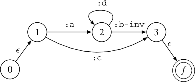
NFA, DFA and minimal DFA produced for the RPQ ${({:p}^{*} / {:p}^{*})}^{*}$ .

Because property paths without inverses and negated property sets are regular expressions, and any regular expression can be transformed into a finite automaton, and a finite automaton has a graph-like structure, we opt to represent property paths based on finite automata. This approach allows us to apply known normal forms for finite automata, providing, in turn, a normal form for RPQs, i.e., property paths without inverses or negated property sets; it further provides partial canonicalisation in the case of full property paths. Another benefit of this approach is that the automaton can be converted straightforwardly into RDF and used for the graph representation.

Given an RPQ, we apply the following process:

we construct a non-deterministic finite automaton (NFA) based on Thompson’s construction for transforming regular expressions to NFAs [59];

we convert this NFA into a deterministic finite automaton (DFA) by a standard subset expansion (the resulting DFA may be exponential on the number of states in the NFA);

we perform a minimisation of the DFA using Hopcroft’s algorithm [29], which produces a canonical DFA such that all regular expressions that express the same language will produce the same DFA (modulo isomorphism on states).

We now provide an example to illustrate the process.

Example 7.4.

Consider an RPQ (:p*/:p*)*. In Fig. 5 we provide an example of the corresponding NFA produced by Thompson’s algorithm, the DFA produced by subset expansion, and the minimal DFA produced by Hopcroft’s algorithm.

The minimal DFA produced by Hopcroft’s algorithm for the RPQ e can then be encoded as an r-graph $R (e)$ where each state is assigned a fresh blank node, and transitions are labelled with their predicate IRI.

In order to generalise this process to full property paths, we must also support inverses and negated property sets. For inverses, we initially attempt to eliminate as many inverses as possible; for example, ^(^:p)* would be rewritten to simply :p* Thereafter, any remaining inverses or negated property sets are represented with a canonical IRI; for example, ^:p* becomes :p-inv*. Thus the property path again becomes a regular expression, and is converted into a DFA using the aforementioned process. It is worth noting that the resulting DFA may not be canonical, and may thus miss equivalences between property paths (e.g., :p*/^p*, ^:p*/p* and (:p|^p)* should all be equivalent, but are not when represented as :p*/:p-inv*, :p-inv*/:p* and (:p|:p-inv)*, respectively). The r-graph can then be computed as before, where for a negated property set $e =!(p_{1} | \dots | p_{n})$ , we also add: $\begin{array}{l} R (e) = & {(ι (e), a, :notOneOf), \\ (ι (e), :arg, ι (p_{1})), \dots, (ι (e), :arg, ι (p_{n}))} . \end{array}$

We will discuss the inverse mapping from the minimal DFA back to a path expression in Section 7.4.

7.3. Minimisation and canonicalisation

Minimisation is applied only to BGPs and UBGPs that are contained within the larger query in the r-graph, considering any variable appearing outside of the BGP or union as a projected variable. We apply canonicalisation on the entire r-graph as before, computing a deterministic labelling for blank nodes.

7.4. Inverse mapping

The inverse mapping is defined analogously such that $R^{-} (R (Q)) = Q$ , with one exception: property paths. This is because we do not represent property paths syntactically in the r-graph, but rather convert them to a minimal DFA, from which we must construct the property path once again. In order to construct the property path from the minimal DFA, we convert it into a regular expression by using the state elimination method [8], from which we can retrieve a normalised RPQ. Finally the inverse and negated property set IRIs are substituted accordingly (if present).

Example 7.5.
Consider the following DFA:

The first step consists in transforming this DFA into an equivalent NFA by introducing a new initial state $q_{0}$ and a single accepting state $q_{f}$ . We add an ϵ transition from $q_{0}$ to $q_{1}$ , and from all accepting states to $q_{f}$ .

To eliminate a state $q_{a}$ we have to replace all transitions that pass through $q_{a}$ . Assuming there exists a path between $q_{i}$ and $q_{j}$ that passes through $q_{a}$ , we define the new transition $e_{i j}$ as $e_{i j} = (e_{i a} / e_{a}^{} / e_{a j}) | e_{i j}^{'}$ . In this expression, we have $e_{i a}$ , the transition from $q_{i}$ to $q_{a}$ , followed by zero or more instances of $e_{a}$ , which represents any self-loops in $q_{a}$ , or ϵ if no such self-loops exist. This is then followed by $e_{a j}$ , the transition from $q_{a}$ to $q_{j}$ . Finally, we have to consider the fact that there may have already been a path from $q_{i}$ to $q_{j}$ , denoted here by $e_{i j}^{'}$ ; hence we append $\dots | e_{i j}^{'}$ to the expression to include the existing transition.

We now eliminate $q_{1}$ following this process. Since $q_{1}$ has no self-loops and there are no existing paths between $q_{0}$ and $q_{2}$ , these terms are excluded from the expression. Then $e_{02} = (e_{01} / e_{1}^{} / e_{12}) | e_{02} = ϵ / :a = :a$ , and $e_{03} = (e_{01} / e_{1}^{} / e_{13}) | e_{03} = ϵ / :c = :c$ .

Next we eliminate $q_{2}$ . In this case, $q_{2}$ does have a self-loop, and there exists a transition between $q_{0}$ and $q_{3}$ so the expression is as follows: $e_{03} = (e_{02} / e_{2}^{} / e_{23}) | e_{03} = (:a / {:d}^{} / :b-inv) ∣ :c$ .

We now eliminate $q_{3}$ . In this case:

Finally, we substitute the IRI :b-inv for the inverse expression ^:b, yielding $(:a / {:d}^{} /^:b) | :c$ .

7.5. Soundness, completeness and incompleteness

Given a SPARQL 1.1 query Q, the canonicalisation procedure is then defined by $R^{-} (L (M (R (A (Q)))))$ . We now discuss some formal properties of this procedure.

7.5.1. Soundness and completeness for EMQs

First we look at the case of EMQs, and ask if the extended canonicalisation procedure is sound and complete for this fragment.

Lemma 7.1.
Given two EMQs $Q_{1}$ and $Q_{2}$ , it holds that $Q_{1} ≅ Q_{2}$ if and only if $\begin{matrix} R^{-} (L (M (R (A (Q_{1}))))) = R^{-} (L (M (R (A (Q_{2}))))) . \end{matrix}$

Please see Appendix A.2.1 for the proof.
7.5.2. Soundness for SPARQL 1.1

Next we show that the process is sound for queries in the full SPARQL 1.1 query language.

Lemma 7.2.
For a SPARQL 1.1 query Q, it holds that: $\begin{matrix} R^{-} (L (M (R (A (Q))))) ≅ Q . \end{matrix}$

Please see Appendix A.2.2 for the proof.
7.5.3. Complexity

In terms of the complexity of (partially) canonicalising queries with these additional features, if we assume that the size of the input query Q is in $O (n)$ , where n is the number of unique triple patterns and path patterns in Q, then the complexity remains bounded by that of canonicalising monotone queries: $O (2^{c n log n})$ for some constant $c > 0$ . This assumes that features of the query that do not involve triple or path patterns (e.g., BIND, VALUES, FILTER, etc.) are of bounded size and bounded in number, while path expressions are of bounded length. This may be an oversimplification.

We may rather consider the “token length” of the query, which is the number of terminals – RDF terms, variables, keywords, etc. – appearing in the syntax of the query. In this case, we must additionally consider the costs of computing a normal form for RPQs. Given an RPQ of length l, which includes the number of non-parenthetical symbols (including IRIs, *, +, |, /) Thompson’s construction creates an NFA of size $O (l)$ . Subset expansion may then create a DFA with $O (2^{l})$ states that remains exponential after minimisation. This will result in an exponentially-sized representation of the RPQ. Minimisation is only applied on (U)BGPs, and thus does not apply on this representation. However, canonical labelling will occur on this representation, where assuming again a brute-force method in the order of $O (b!)$ for b the number of blank nodes, we now have a complexity of $O (2^{l}!)$ for canonicalising the RPQ representation graph of a property path of length l, and given that we may have n such property paths, where n is the number of triple patterns and path expressions, this generates a cost of $O ((c n 2^{l})!)$ for canonically labelling a navigational graph pattern, which we can add to the cost for monotone queries: $O ((c n 2^{l})! + (c n 3^{n / 3})!)$ , where l is the length of the longest property path, n is the number of triple patterns and path patterns, and $c > 0$ is some constant to account for the additional “syntactic” blank nodes that appear in the r-graph.

7.5.4. Incompleteness for SPARQL 1.1

We provide some examples of incompleteness to illustrate the limitations of the canonicalisation process for the full SPARQL 1.1 language.

We start with filters, which, when combined with a particular graph pattern, may always be true, may never be true, may contain redundant elements, etc.; however, detecting such cases can be highly complex.

Example 7.6.
Consider the following example: The FILTER here will always return false as the predicate in an RDF graph must always be an IRI. Thus the query is unsatisfiable and thus ideally would be rewritten to $Q_{\emptyset}$ ; however, we do not consider the semantics of filter functions (other than boolean combinations).

Note that reasoning about filters is oftentimes far from trivial. Consider the following example: This query is unsatisfiable because predicates must be IRIs, and IRIs must always contain a colon (to separate the scheme from the hierarchical path) [20].

Next we consider issues with property paths.
Example 7.7.
Consider the following example: Clearly this is equivalent to: But also to: Currently we rewrite concatenation, inverse and disjunction in paths (not appearing within a recursive expression) to UCQ features. This means that we currently capture equivalence between the first and second query, but not the first and third.

Other examples are due to inverses, or negated property sets; consider for example: This is equivalent to: However, we do not consider the semantic relation between the expressions !(:parent) and :parent.

Incompleteness can also occur due to negation, which is complicated by the ambiguities surrounding NOT EXISTS as discussed in Section 3.10. We have postponed algebraic rewritings involving negation until this issue is officially resolved.

Incompleteness can also occur while normalising well-designed query patterns with OPTIONAL.
Example 7.8.
Consider the query $Q_{1}$ : Since AND is commutative, this is equivalent to $Q_{2}$ : If we rewrite each well-designed pattern by pushing the OPTIONAL operators outside, we obtain the following equivalent query for $Q_{1}$ : and, analogously, for $Q_{2}$ : However, in the general case it does not hold that $[[Q_{1} OPT Q_{2}] OPT Q_{3}] \equiv [[Q_{1} OPT Q_{3}] OPT Q_{2}]$ , and thus we do not capture these equivalences.

We could list an arbitrary number of ways in which arbitrary features can give rise to unsatisfiability or redundancy, or where queries using seemingly different features end up being equivalent. We could likewise provide an arbitrary number of rewritings and methods to deal with particular cases. However, any such method for canonicalising SPARQL 1.1 queries will be incomplete. Furthermore, many such “corner cases” would be rare in practice, where dealing with them might have limited impact. We then see two interesting directions for future work to address these limitations:
Use query logs or other empirical methods to determine more common cases that this query canonicalisation framework may miss and implement targeted methods to deal with such cases.

Extend the query fragment for which sound and complete canonicalisation is possible; an interesting goal, for example, would be to explore EMQs with full property paths (such queries are similar to C2RPQs [34], for which containment and related problems are decidable).

8. Experiments

In these experiments, we wish to address two principal questions, as follows:

How is the performance of the canonicalisation procedure in terms of runtime? Which aspects of the procedure take the most time? What kinds of queries are most expensive?

How many more additional congruent queries can the procedure find in real-world logs versus baseline methods? Which aspects of the procedure are most important for increasing the number of congruent queries detected?

With respect to the first question, we might expect poor performance given that the worst-case of the algorithm is super-exponential. However, this is a worst-case analysis with respect to the size of the query, where queries in practice are often relatively small and simple. Hence our hypothesis is that although there exist queries for which canonicalisation is not computationally feasible in theory, it should run efficiently (in fractions of a second) for the majority of real-world queries in practice (as found in public query logs).

With respect to the second question, most of our expected use-cases benefit from being able to find a wider range of congruent, real-world queries, as found in public query logs; for example, in the case of caching, finding more congruent queries will translate into higher cache hit rates. Thus it is of interest to see how many additional congruent queries our canonicalisation procedure can find from public query logs when compared with baseline (syntactic) methods, and in particular, which parts of the procedure have the most impact in terms of finding more congruent queries. In general, we hypothesise that canonical labelling will be an important component as variable naming would likely be a common variation in real-world queries; on the other hand, we hypothesise that minimisation will be less impactful in terms of finding more congruent queries as we expect few real-world queries to contain the types of redundancy dealt with in Section 6.3.

We thus design a number of experiments over real-world and synthetic queries in order to address these questions and evaluate our expectations.

8.1. Implementation: QCan

We have implemented the canonicalisation procedure in a system that we call QCan written in Java. The system uses Jena ARQ [38] for query parsing and processing. Algebraic rewritings are implemented on top of the query algebra that Jena ARQ provides. Constructing the r-graph is likewise implemented on top of Jena. Minimisation is conducted by using the blabel system [28] to compute the core of RDF graphs representing BGPs, thereafter implementing containment checks across BGPs using ASK queries evaluated in Jena. Finally canonical labelling is implemented using blabel [28]. All other aspects of the procedure are implemented directly in QCan, including the steps involving the representation and manipulation of property paths as automata. The source code of QCan, along with a suite of congruence test-cases, are available online at: http://github.com/RittoShadow/QCan. The machine used for these experiments has 12 Intel^® Xeon^® 1.9GHz processors, and runs on Devuan GNU/Linux 2.1, with a maximum heap size of 10GB.

8.2. Real-world query logs

In order to test our algorithm in a real-world setting, we used two query log datasets: the LSQ dataset [52],19

¹⁹
https://aksw.github.io/LSQ/

which itself contains queries from DBpedia, Linked Geo Data, RKB Explorer/Endpoint and Semantic Web Dog Food logs; and Wikidata logs [37] (Interval 7; organic queries).20

²⁰

https://iccl.inf.tu-dresden.de/web/Wikidata_SPARQL_Logs/en

With respect to the datasets:

DBpedia [35] (DBp) is an RDF dataset extracted principally from Wikipedia, with the main source of content being info-boxes.

LinkedGeoData [56] (Geo) is an RDF dataset that contains spatial data extracted from the OpenStreetMap [23] project.

The RKB Endpoint (REn) and Explorer (REx) datasets [21] primarily pertain to cultural and heritage data from the British Museum.

Semantic Web Dog Food (SWDF) [39] was a dataset that is now part of the Scholarlydata dataset [40], containing information about scholarly publications and conferences.

Wikidata [61] (WD) is a collaboratively-edited knowledge graph that complements the projects of Wikimedia with central, structured content.

Table 24

Distribution of queries using SPARQL features in the query logs; we mark features new to SPARQL 1.1 with an asterisk

Feature	DBp	Geo	REn	REx	SWDF	WD	All
BGP	424,328	842,794	169,425	335,450	112,398	861,383	2,745,778
Distinct	192,168	5,477	147,575	210,058	57,195	538,878	1,151,351
And	58,952	78,575	19,355	34,180	54,702	751,243	997,007
Mods	4,576	412,343	40,957	80,655	60,199	321,239	919,969
Opt	31,211	19,914	9,741	23,587	27,824	343,838	456,115
Filter	200,001	125,849	8,974	14,938	4,716	92,807	447,285
Service*	0	0	0	0	0	406,990	406,990
Union	89,766	49,299	1,653	5,550	32,459	57,029	235,756
Paths*	0	0	96	192	37	268,530	268,855
Bind*	0	0	0	19,641	15,307	71,102	106,050
Agg*	0	0	0	16,444	10,268	42,777	69,489
Values*	0	174	0	0	83	55,037	55,294
Minus*	0	0	0	192	25	5,700	5,917
Total	424,362	842,794	169,617	335,833	112,470	868,993	2,754,069

All of these datasets have public SPARQL endpoints that receive queries from users over the Web. These queries have been published as the Wikidata and LSQ logs for research purposes. Table 24 contains the distribution of features in each of the query sets in our real-world setting. In total we consider 2.8 million queries for our experiments. Despite the fact that BGPs are equivalent to joins of triple patterns, we only count as “and” those joins for features other than triple patterns. We further gather together under “mods” the solution modifiers ORDER BY, LIMIT, OFFSET and projection. We observe that BGPs are present in almost all queries, which is an expected result. Features new to SPARQL 1.1 are used more rarely in the LSQ logs, but this is likely because these logs predate the release of the standard; such features are quite widely used in the more recent Wikidata logs. The large use of Service on Wikidata relates to the use of the custom label service offered by the endpoint as a syntactic convenience to help choose language preferences. With respect to the use of property paths, many are quite simple, usually used to find objects of a certain class or its transitive subclasses. Further details of these queries can be found in analyses by Saleem et al. [52], Malyshev et al. [37], Bonifati et al. [7], etc.

Fig. 6.

Runtimes for each step of the canonicalisation algorithm.

8.2.1. Canonicalisation runtimes

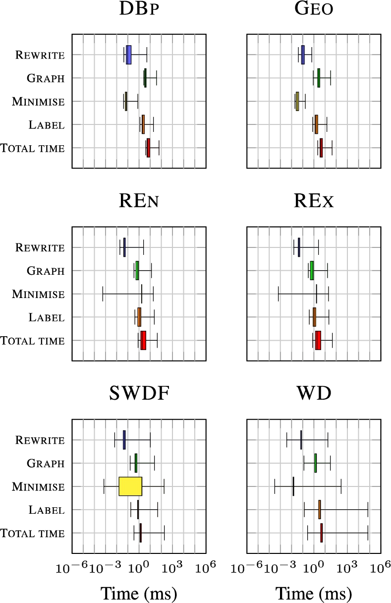
We now present the runtimes for canonicalising the queries of the aforementioned logs. All queries in all six logs were successfully canonicalised. The results in Fig. 6 indicate that the fastest queries to canonicalise take around 0.00025 seconds, median times vary from 0.00084 seconds (REn) up to 0.00206 seconds (WD), while max times vary from 0.12 seconds (SWDF) up to 71 seconds (WD). The slowest part of the process, on average, tended to be the canonical labelling, though in the case of REn and REx, the graph construction was slightly slower on average.

Fig. 7.

Runtimes for each step of the canonicalisation algorithm (considering queries with some SPARQL 1.1 feature).

Figure 7 shows the runtimes for the canonicalisation of the queries in the aforementioned logs, limited to those that contain features introduced in SPARQL 1.1. Notably the ranges of runtimes of DBp, Geo, REn, and REx are much more stable, and present much less variance than the same runtimes for the full datasets. On the other hand, SWDF and WD present similar minimum and maximum runtimes than the full datasets, but the runtimes in the interquartile range are far more stable than those in the full datasets. This suggests that the addition of queries with features introduced in SPARQL 1.1 do not add a significant overhead to the performance of the algorithm.

Fig. 8.

R-graph sizes (number of nodes) for each set of queries; the value on the right indicates the maximum size.

Figure 8 shows that the WD set of queries produces the largest r-graphs, with the largest graph containing 3,456 nodes (WD). This is consistent with the results in Fig. 6 since the total runtimes for WD queries can be much higher than those of the other query sets.

Fig. 9.

Runtimes for queries grouped by selected features.

The results in Fig. 9 show the runtimes for all query sets grouped by the features they use (at least once, possibly in conjunction with other features). We include SPARQL 1.0 features along with property paths for those logs using such features. These results indicate that queries containing UNION tend to take a longer time to process; i.e., it is the most computationally challenging feature to deal with in these queries. This is an expected result since the rewriting step may cause an exponential blow-up on the number of basic graph patterns in a monotone fragment of a query. Since most real world queries are not in a UCQ form, but rather contain combinations of joins and unions, it is likely that any query that contains unions will produce larger r-graphs than those without any unions. We also see that OPTIONAL is an expensive feature, particularly for the Geo dataset. However, looking into the Geo results in more detail, most of the queries with OPTIONAL appear to come from a single agent – an application using the SPARQL endpoint as a backend – and also feature numerous disjunctive filters (using bound(·) over multiple OPTIONAL clauses) that are rewritten into UNION, which is then the underlying reason that the queries are slower. This result – relating to the requests of a single prolific agent – can thus be considered something of an outlier.

8.2.2. Duplicates found

We now look at the number of duplicates found, where we compare the following methods:

Raw

The raw query string is used, without any kind of normalisation.

Parse

The raw query string is parsed using Jena ARQ into its query algebra, and then serialised back into concrete SPARQL syntax.

Label

The raw query string is parsed using Jena ARQ into its query algebra, the r-graph is constructed and canonically labelled, and then serialised back into concrete SPARQL syntax.

Rewrite

The raw query string is parsed using Jena ARQ into its query algebra, the query is rewritten per the algebraic rules, the r-graph is constructed and canonically labelled, and then serialised back into concrete SPARQL syntax.

Full

The raw query string is parsed using Jena ARQ into its query algebra, the query is rewritten per the algebraic rules, the r-graph is constructed, minimised, canonically labelled, and then serialised back into concrete SPARQL syntax.

Table 25
Total number of duplicates found by each method

Query set Raw Parse Label Rewrite Full

DBp 250,940 251,283 251,315 251,315 251,315

Geo 723,116 736,331 739,695 739,700 739,702

REn 142,032 143,523 144,007 144,007 144,008

REx 299,892 301,419 301,910 301,910 301,911

SWDF 53,061 53,263 53,388 53,388 53,388

WD 683,132 686,453 687,654 687,751 687,760

Query set	Raw	Parse	Label	Rewrite	Full
DBp	250,940	251,283	251,315	251,315	251,315
Geo	723,116	736,331	739,695	739,700	739,702
REn	142,032	143,523	144,007	144,007	144,008
REx	299,892	301,419	301,910	301,910	301,911
SWDF	53,061	53,263	53,388	53,388	53,388
WD	683,132	686,453	687,654	687,751	687,760

Table 26

Most duplicates of a single query found by each method

Query set	Raw	Parse	Label	Rewrite	Full
DBp	5,464	5,514	5,514	5,514	5,514
Geo	22,582	31,379	40,744	40,744	40,744
REn	3,814	3,814	3,814	3,814	3,814
REx	14,690	14,910	14,910	14,910	14,910
SWDF	2,388	2,633	4,938	4,938	4,938
WD	232,339	232,339	232,339	232,339	232,339

Tables 25 and 26 denote the total number of duplicate (congruent) queries found, and the most duplicates found for a single query. In general, there is a high number of exact duplicate query strings, possibly from the same query being sent many times to refresh the results. Thereafter, the number of duplicates found either remains the same or increases in each successive algorithm. In particular, excluding duplicate query strings (Raw), the highest increase occurs with Parse and thereafter Label, with WD being the query set for which the most additional duplicates are found with these methods, where the duplicates detected increase by a few thousand in each step. In the other query sets this increase is less pronounced. In addition, there is almost no difference beyond Label, meaning that algebraic rewritings and minimisation find very few additional congruent queries in these logs.

8.3. Comparison with existing systems

In this section, we compare the runtime performance of our algorithm with existing systems that can perform pairwise SPARQL containment checks. We provide an overview of these tools in Table 27. In our experiments, we consider SA [36] and JSAG [58] as they support cyclic queries. The queries used are part of the test suite designed by Chekol et al. [13] as part of their experiments. These correspond to two sets of queries: one of CQs without projection, and one of UCQs with projection. As discussed in Section 5, the SA and JSAG systems are not analogous to ours. We focus on query equivalence and congruence, and not on containment; conversely, SA and JSAG support containment. On the other hand, we compute a canonical form of a query, whereas SA and JSAG focus on pairwise checks (though JSAG offers indexing approaches based on constants in the query and isomorphic DAGs). Our approach is sound and complete for UCQs under both bag and set semantics; conversely, SA only considers set semantics, while JSAG focuses on detecting sub-graph isomorphisms between algebraic expressions under bag semantics. In the case of CQs without projection, checking containment is tractable (see Table 16), and quite trivial, requiring checking that one BGP is set-contained in the other.

Table 27
UCQ features supported by SPARQL Algebra (SA), Alternating Free two-way μ-calculus (AFMU), Tree Solver (TS) and Jena-SPARQL-API Graph-isomorphism (JSAG); note that ABGP denotes Acyclic Basic Graph Patterns

Method ABGP BGP Projection Union

SA ✓ ✓

AFMU ✓ ✓ ✓

TS ✓ ✓ ✓

JSAG ✓ ✓ ✓ ✓

QCan ✓ ✓ ✓ ✓

Method	ABGP	BGP	Projection	Union
SA	✓	✓
AFMU	✓		✓	✓
TS	✓		✓	✓
JSAG	✓	✓	✓	✓
QCan	✓	✓	✓	✓

Fig. 10.

Runtimes for JSAG, SA and QCan.

Figure 10 shows the runtimes for our comparison of both containment checkers and our method (QCan). Note that there are no values for SA with UCQs because the UCQ set uses projection and SA does not support queries with projection. The results indicate that most queries for SA and JSAG take between one and ten milliseconds, whereas most queries under our method take between ten and one hundred milliseconds. In terms of the slowest queries, our method is faster than JSAG but slower than SA.

In general, the conclusion is that our method is slower for testing equivalence than existing containment checkers, but this is perhaps not surprising as our approach addresses the more difficult problem of first computing a canonical form for both input queries, and further considers congruence rather than the more trivial case of equivalence where variable names are fixed. Furthermore, once these canonical forms are computed, equivalence classes of congruent queries can be found in constant time using simple data structures (e.g., (ideal) hashing of the canonical query strings). If we estimate that our system is 10 times slower to canonicalise two queries than these systems can perform a pairwise check (per Fig. 10), QCan will begin to outperform these systems for partitioning a set of 11 or more queries by equivalence (or congruence); in the case of 11 queries, these systems must perform $(\binom{11}{2}) = 55$ pairwise checks (in the worst case), while QCan will canonicalise 11 queries and partition them in constant time (in the best and the worst case). The time savings thereafter grow quadratically.

8.4. Stress test

With the exception of some outliers, most queries that we have evaluated thus far have been canonicalised in fractions of a second. On the other hand, we know that our algorithms are super-exponential in the worst case. Such cases may occur when we have monotone queries that are in conjunctive normal form (i.e., consisting of joins of unions), in which case our UCQ normal form can be exponential in size, upon which we perform further potentially exponential processes. In order to stress-test our method and explore such worst cases, we run the following experiment.

For this experiment, we generate queries of the form $AND (U_{1}, \dots, U_{m})$ where each union pattern is of the form $U_{i} = UNION (t_{1}, \dots, t_{k})$ , and each triple pattern is of the form $t_{j} = (s_{j}, {:p}_{j}, o_{j})$ , where $s_{j}$ and $o_{j}$ are variables randomly selected from a predetermined set of $m + k$ variables, and ${:p}_{j}$ is an IRI randomly selected from a predetermined set of m IRIs. The UCQ normal form for this query will consist of a union of $k^{m}$ BGPs, each containing m triple patterns. Finally, we project a random subset of the set of variables that appear in the query, making sure to project at least one variable.

Fig. 11.

Times for UCQ stress tests.

Figure 11 shows the times for each step of the canonicalisation procedure on the synthetic UCQs. On the x-axis we increase k (the base of the exponent), while across the different series we increase m (the exponent). The y-axis is shown in log scale. We see that for the UCQ rewriting, graph construction and minimisation steps, the higher series (representing an increasing exponent) diverge further and further as the x-axis increases (representing an increasing base). On the other hand, the differences in times for canonical labelling are less pronounced since the minimisation process reduces the r-graphs significantly due to the regular construction of the queries. The slowest queries tested ( $k = 9$ , $m = 4$ ) take around 4.1 hours to canonicalise considering all steps. Increasing k and/or m further would quickly lead to unmanageable runtimes and, eventually, out-of-memory exceptions.

These results illustrate the poor worst-case behaviour of our canonicalisation procedure, particularly when considering queries with joins of many unions. However, as shown by the results presented in Section 8.2, virtually no queries in our real-world setting caused this worst-case behaviour.

9. Conclusion

In this paper, we have presented a formal semantics of SPARQL 1.1 and a canonicalisation procedure that produces a deterministic query string modulo congruence (equivalence modulo variable naming). This procedure involves the application of algebraic rewritings of the query, the representation of the query as a graph, the minimisation of the query in order to remove redundancy, and finally the canonical labelling of the graph in order to produce canonical variable names based on the structure of the graph. We have proven this procedure to be sound and complete with respect to “extended monotone queries” under bag and set semantics, i.e., queries that can be rewritten to the features involving BGPs, joins, unions, projection, and distinct. We have further extended this procedure to provide sound and incomplete canonicalisation of the queries under the full SPARQL 1.1 language.

Despite the super-exponential worst-case complexity of our procedure, the experimental results indicate that our method is efficient for most queries, running in a fraction of a second – in the median case – over millions of queries from real-world logs; the slowest query to canonicalise took just over a minute. Such results are achieved because most real-world queries tend to be relatively small and simple. In this analysis, we determined that the canonical labelling is the step that takes the longest time on average. We further found that the UNION feature is the most costly to canonicalise in general, with OPTIONAL also proving costly in some cases. Comparing the performance of our method for finding equivalent queries versus existing containment checkers, we find that our method is indeed slower, but produces a canonical form that thereafter allows for constant-time detection of congruent queries in large sets of queries. Running stress-tests over queries featuring joins of unions of increasing size, we have confirmed that our procedure quickly becomes inefficient, taking hours to canonicalise four joins of unions with nine triple patterns each.

We have further confirmed that our procedure allows for detecting additional congruent queries over real-world logs versus baseline methods. We first observed that the vast majority of congruent queries are actually syntactically identical in terms of raw query strings, likely due to clients reissuing precisely the same query in order to intermittently refresh results. Of our canonical procedures, canonical labelling is the most important for finding additional congruent queries. On the other hand, minimisation and algebraic rewritings – though necessary to ensure completeness for monotone queries – lead to finding only a very small fraction of additional congruent queries. This would tend to suggest that in a practical caching system, where completeness can be traded for efficiency, it may be sufficient to apply canonical labelling without algebraic rewritings and minimisation. However, minimisation may be useful in cases where completeness is an important criterion. Also, in certain setting, queries with redundancy may be automatically generated; an interesting use-case along these lines is that of ontology-based data access (OBDA) [63], where rewritings may produce queries (typically UCQs) with redundancies that are inefficient to evaluate over large graphs.

With respect to future directions, a natural continuation of this work is to explore larger fragments of SPARQL 1.1 for which sound and complete canonicalisation can be performed. In particular, we have already begun to investigate such procedures for a fragment akin to UC2RPQs. At first glance, this should be analogous to the minimisation and canonicalisation of basic graph patterns and unions, where property paths are represented as automata and we can check for containment of automata to find redundant path patterns. However, we have already found that this requires entailment of paths with inverses, which is not as straightforward as checking for containment [34].

SPARQL 1.2 is on the horizon. We believe that the formal semantics of SPARQL 1.1 defined herein may serve as a useful reference for the standardisation effort. If the semantics of FILTER (NOT) EXISTS is clarified as part of SPARQL 1.2, it would also be of interest to (partially) capture equivalences between the negation features of SPARQL. With respect to new features, our canonicalisation procedure should be extensible to SPARQL 1.2 following similar processes, though such canonicalisation cannot be complete.

Finally, we are currently exploring use-cases for our canonicalisation procedure in the context of two ongoing projects: one relating to caching, and one relating to query answering. Regarding caching, we have seen that most congruences in real-world query logs are exact (syntactic) duplicates; however, rather than considering congruencies between full queries, a more promising approach for caching is to mine common sub-queries, where canonicalisation can be used for such purposes. In the context of question answering, we can also use canonicalisation in order to normalise training data for sequence-to-sequence models that translate natural language to SPARQL queries. An important future line of research is then to explore and evaluate the benefits of SPARQL canonicalisation in the context of these and further use-cases.

Online material We provide code and other material online at: http://github.com/RittoShadow/QCan. A demo is available at: http://qcan.dcc.uchile.cl.

Footnotes

Acknowledgements

This work was supported by Fondecyt Grant No. 1181896 and by ANID – Millennium Science Initiative Program – Code ICN17_002. We would also like to thank the reviewers of the conference and journal versions of this paper for useful comments that helped to improve this work.

Proofs

References

F.N.

Afrati ,

Damigos and

Gergatsoulis , Query containment under bag and bag-set semantics, Inf. Process. Lett.110(10) (2010), 360–369. doi:10.1016/j.ipl.2010.02.017.

Alkhateeb ,

J.-F.

Baget and

Euzenat , Extending SPARQL with regular expression patterns (for querying RDF), Web Semantics7(2) (2009), 57–73. doi:10.1016/j.websem.2009.02.002.

Angles ,

Arenas ,

Barceló ,

Hogan ,

Reutter and

Vrgoč , Foundations of modern query languages for graph databases, ACM Computing Surveys50(5) (2017), 68. doi:10.1145/3104031.

C.B.

Aranda ,

Hogan ,

Umbrich and

Vandenbussche , SPARQL Web-querying infrastructure: Ready for action? in: International Semantic Web Conference (ISWC), Vol. 8219, Springer, 2013, pp. 277–293. doi:10.1007/978-3-642-41338-4_18.

Arenas and

Pérez, Federation and navigation in SPARQL 1.1, in: Reasoning Web Summer School, LNCS, Vol. 7487, Springer, 2012, pp. 78–111. doi:10.1007/978-3-642-33158-9_3.

Arenas and

Ugarte , Designing a query language for RDF: Marrying open and closed worlds, ACM Trans. Database Syst.42(4) (2017), 21:1–21:46. doi:10.1145/3129247.

Bonifati ,

Martens and

Timm , An analytical study of large SPARQL query logs, VLDB J.29(2–3) (2020), 655–679. doi:10.1007/s00778-019-00558-9.

J.A.

Brzozowski and

E.J.

McCluskey , Signal flow graph techniques for sequential circuit state diagrams, in: IEEE Transactions on Electronic Computers, 1963, pp. 67–76. doi:10.1109/PGEC.1963.263416.

Castillo and

Leser , Selecting materialized views for RDF data, in: International Conference on Web Engineering (ICWE), Workshops,

Daniel and

F.M.

Facca , eds, Lecture Notes in Computer Science, Vol. 6385, Springer, 2010, pp. 126–137. doi:10.1007/978-3-642-16985-4_12.

10.

Chakraborty ,

Lukovnikov ,

Maheshwari ,

Trivedi ,

Lehmann and

Fischer , Introduction to Neural Network based Approaches for Question Answering over Knowledge Graphs, 2019, CoRR, http://arxiv.org/abs/1907.09361abs/1907.09361.

11.

A.K.

Chandra and

P.M.

Merlin , Optimal implementation of conjunctive queries in relational data bases, in: Symposium on Theory of Computing (STOC),

J.E.

Hopcroft ,

E.P.

Friedman and

M.A.

Harrison , eds, ACM, 1977, pp. 77–90. doi:10.1145/800105.803397.

12.

Chaudhuri and

M.Y.

Vardi , Optimization of Real Conjunctive Queries, in: Principles of Database Systems (PODS), ACM Press, 1993, pp. 59–70. doi:10.1145/153850.153856.

13.

M.W.

Chekol ,

Euzenat ,

Genevès and

Layaïda , SPARQL Query Containment Under SHI Axioms, in: AAAI Conference on Artificial Intelligence, AAAI Press, 2012.

14.

M.W.

Chekol ,

Euzenat ,

Genevès and

Layaïda , Evaluating and benchmarking SPARQL query containment solvers, in: International Semantic Web Conference (ISWC),

Alani ,

Kagal ,

Fokoue ,

Groth ,

Biemann ,

J.X.

Parreira ,

Aroyo ,

N.F.

Noy ,

Welty and

Janowicz , eds, Lecture Notes in Computer Science, Vol. 8219, Springer, 2013, pp. 408–423. doi:10.1007/978-3-642-41338-4_26.

15.

Chu ,

Murphy ,

Roesch ,

Cheung and

Suciu , Axiomatic foundations and algorithms for deciding semantic equivalences of SQL queries, Proc. VLDB Endow.11(11) (2018), 1482–1495. doi:10.14778/3236187.3236200.

16.

Chu ,

Wang ,

Weitz and

Cheung , Cosette: An automated prover for SQL, in: Conference on Innovative Data Systems Research (CIDR), 2017, www.cidrdb.org.

17.

Cohen ,

Nutt and

Serebrenik , Rewriting aggregate queries using views, in: SIGACT-SIGMOD-SIGART Symposium on Principles of Database Systems (PODS), ACM Press, 1999, pp. 155–166. doi:10.1145/303976.303992.

18.

Cyganiak , A relational algebra for SPARQL, 2005, http://shiftleft.com/mirrors/www.hpl.hp.com/techreports/2005/HPL-2005-170.pdf.

19.

Cyganiak ,

Wood and

Lanthaler , RDF 1.1 Concepts and Abstract Syntax, 2014. http://www.w3.org/TR/rdf11-concepts/.

20.

Dürst and

Suignard , in: Internationalized Resource Identifiers (IRIs), Vol. 3987, 2005, pp. 1–46. https://tools.ietf.org/html/rfc3987. doi:10.17487/RFC3987.

21.

Glaser ,

Millard and

Jaffri , RKBExplorer.com: A knowledge driven infrastructure for linked data providers, in: European Semantic Web Conference (ESWC), Lecture Notes in Computer Science, Vol. 5021, Springer, 2008, pp. 797–801. doi:10.1007/978-3-540-68234-9_61.

22.

Gutierrez ,

C.A.

Hurtado ,

A.O.

Mendelzon and

Pérez , Foundations of Semantic Web databases, J. Comput. Syst. Sci.77(3) (2011), 520–541. doi:10.1016/j.jcss.2010.04.009.

23.

M.M.

Haklay and

Weber , OpenStreetMap: User-generated street maps, IEEE Pervasive Comput.7(4) (2008), 12–18. doi:10.1109/MPRV.2008.80.

24.

Harris ,

Seaborne and

Prud’hommeaux , 2013, SPARQL 1.1 Query Language, http://www.w3.org/TR/sparql11-query/.

25.

Hayes and

P.F.

Patel-Schneider , RDF 1.1 Semantics, 2014, http://www.w3.org/TR/2014/REC-rdf11-mt-20140225/.

26.

Heath and

Bizer , Linked Data: Evolving the Web into a Global Data Space, Vol. 1, Morgan & Claypool, 2011, pp. 1–136. ISBN 9781608454310.

27.

Hernández ,

Gutiérrez and

Angles , The Problem of Correlation and Substitution in SPARQL – Extended Version, 2018, CoRR, http://arxiv.org/abs/1801.04387abs/1801.04387.

28.

Hogan , Canonical forms for isomorphic and equivalent RDF graphs: Algorithms for leaning and labelling blank nodes, ACM TOW11(4) (2017), 22:1–22:62. doi:10.1145/3068333.

29.

Hopcroft , An n log n algorithm for minimizing states in a finite automaton, in: Theory of Machines and Computations, Elsevier, 1971, pp. 189–196. doi:10.1016/B978-0-12-417750-5.50022-1.

30.

Y.E.

Ioannidis and

Ramakrishnan , Containment of conjunctive queries: Beyond relations as sets, ACM Trans. Database Syst.20(3) (1995), 288–324. doi:10.1145/211414.211419.

31.

T.A.

Junttila and

Kaski , Engineering an efficient canonical labeling tool for large and sparse graphs, in: Workshop on Algorithm Engineering and Experiments (ALENEX), SIAM, 2007. doi:10.1137/1.9781611972870.13.

32.

Kaminski ,

E.V.

Kostylev and

B.C.

Grau , Query nesting, assignment, and aggregation in SPARQL 1.1, ACM Trans. Database Syst.42(3) (2017), 17:1–17:46. doi:10.1145/3083898.

33.

Kharlamov ,

Hovland ,

M.G.

Skjæveland ,

Bilidas ,

Jiménez-Ruiz ,

Xiao ,

Soylu ,

Lanti ,

Rezk ,

Zheleznyakov ,

Giese ,

Lie ,

Y.E.

Ioannidis ,

Kotidis ,

Koubarakis and

Waaler , Ontology based data access in statoil, J. Web Semant.44 (2017), 3–36. doi:10.1016/j.websem.2017.05.005.

34.

E.V.

Kostylev ,

J.L.

Reutter ,

Romero and

Vrgoc , SPARQL with property paths, in: International Semantic Web Conference (ISWC), Lecture Notes in Computer Science (LNCS), Vol. 9366, Springer, 2015, pp. 3–18. doi:10.1007/978-3-319-25007-6_1.

35.

Lehmann ,

Isele ,

Jakob ,

Jentzsch ,

Kontokostas ,

P.N.

Mendes ,

Hellmann ,

Morsey ,

van Kleef ,

Auer and

Bizer , DBpedia – a large-scale, multilingual knowledge base extracted from Wikipedia, Semantic Web6(2) (2015), 167–195. doi:10.3233/SW-140134.

36.

Letelier ,

Pérez ,

Pichler and

Skritek , Static analysis and optimization of semantic web queries, ACM Trans. Database Syst.38(4) (2013), 25:1–25:45. doi:10.1145/2500130.

37.

Malyshev ,

Krötzsch ,

González ,

Gonsior and

Bielefeldt , Getting the most out of wikidata: Semantic technology usage in Wikipedia’s knowledge graph, in: Proceedings, Part II, The Semantic Web – ISWC 2018 – 17th International Semantic Web Conference, Monterey, CA, USA, October 8–12, 2018, 2018, pp. 376–394. doi:10.1007/978-3-030-00668-6_23.

38.

McBride , Jena: A Semantic Web toolkit, IEEE Internet Computing6(6) (2002), 55–59. doi:10.1109/MIC.2002.1067737.

39.

Möller ,

Heath ,

Handschuh and

Domingue , Recipes for Semantic Web Dog Food – the ESWC and ISWC Metadata Projects, in: International Semantic Web Conference (ISWC), Lecture Notes in Computer Science, Vol. 4825, Springer, 2007, pp. 802–815. doi:10.1007/978-3-540-76298-0_58.

40.

A.G.

Nuzzolese ,

A.L.

Gentile ,

Presutti and

Gangemi , Conference linked data: The ScholarlyData project, in: International Semantic Web Conference (ISWC), Lecture Notes in Computer Science9982 (2016), 150–158. doi:10.1007/978-3-319-46547-0_16.

41.

Papailiou ,

Tsoumakos ,

Karras and

Koziris , Graph-aware, workload-adaptive SPARQL query caching, in: ACM SIGMOD International Conference on Management of Data,

T.K.

Sellis ,

S.B.

Davidson and

Z.G.

Ives , eds, ACM, 2015, pp. 1777–1792. doi:10.1145/2723372.2723714.

42.

P.F.

Patel-Schneider and

Martin , EXISTStential aspects of SPARQL, in: ISWC 2016 Posters & Demonstrations Track, CEUR Workshop Proceedings, Vol. 1690, CEUR-WS.org, 2016.

43.

Pérez ,

Arenas and

Gutiérrez , Semantics and Complexity of SPARQL, in: International Semantic Web Conference (ISWC), LNCS, Vol. 4273, Springer, 2006, pp. 30–43. doi:10.1007/11926078_3.

44.

Pérez ,

Arenas and

Gutierrez , Semantics and complexity of SPARQL, ACM Trans. Database Syst.34(3) (2009). doi:10.1145/1567274.1567278.

45.

Pichler and

Skritek , Containment and equivalence of well-designed SPARQL, in: Principles of Database Systems (PODS), ACM, 2014, pp. 39–50. doi:10.1145/2594538.2594542.

46.

Polleres , From SPARQL to rules (and back), in: International Conference on World Wide Web (WWW),

C.L.

Williamson ,

M.E.

Zurko ,

P.F.

Patel-Schneider and

P.J.

Shenoy , eds, 2007, pp. 787–796. doi:10.1145/1242572.1242679.

47.

Polleres and

J.P.

Wallner , On the relation between SPARQL1.1 and answer set programming, J. Appl. Non Class. Logics23(1–2) (2013), 159–212. doi:10.1080/11663081.2013.798992.

48.

Prud’hommeaux and

Buil-Aranda , SPARQL 1.1 Federated Query, 2013, https://www.w3.org/TR/sparql11-federated-query/.

49.

Sagiv and

Yannakakis , Equivalences among relational expressions with the union and difference operators, J. ACM27(4) (1980), 633–655. doi:10.1145/322217.322221.

50.

Salas and

Hogan , Canonicalisation of monotone SPARQL queries, in: International Semantic Web Conference (ISWC),

Vrandecic ,

Bontcheva ,

M.C.

Suárez-Figueroa ,

Presutti ,

Celino ,

Sabou ,

Kaffee and

Simperl , eds, Lecture Notes in Computer Science, Vol. 11136, Springer, 2018, pp. 600–616. doi:10.1007/978-3-030-00671-6_35.

51.

Salas and

Hogan , Canonicalisation of Monotone SPARQL Queries, http://aidanhogan.com/qcan/extended.pdf.

52.

Saleem ,

M.I.

Ali ,

Hogan ,

Mehmood and

A.N.

Ngomo , LSQ: The Linked SPARQL Queries Dataset, International Semantic Web Conference (ISWC), Vol. 9367, Springer, 2015, pp. 261–269. doi:10.1007/978-3-319-25010-6_15.

53.

Schmidt ,

Meier and

Lausen , Foundations of SPARQL query optimization, in: International Conference on Database Theory (ICDT),

Segoufin , ed., ACM, 2010, pp. 4–33. doi:10.1145/1804669.1804675.

54.

Schreiber and

Raimond , RDF 1.1 Primer, 2014, http://www.w3.org/TR/rdf11-primer/.

55.

Seaborne and

P.F.

Patel-Schneider , SPARQL EXISTS report, 2019.

56.

Stadler ,

Lehmann ,

Höffner and

Auer , LinkedGeoData: A core for a web of spatial open data, Semantic Web3(4) (2012), 333–354. doi:10.3233/SW-2011-0052.

57.

Stadler ,

Saleem ,

A.N.

Ngomo and

Lehmann , Efficiently pinpointing SPARQL query containments, in: International Conference on Web Engineering (ICWE),

Mikkonen ,

Klamma and

Hernández , eds, Lecture Notes in Computer Science, Vol. 10845, Springer, 2018, pp. 210–224. doi:10.1007/978-3-319-91662-0_16.

58.

Stadler ,

Saleem ,

A.N.

Ngomo and

Lehmann , Efficiently pinpointing SPARQL query containments, in: International Conference Web Engineering (ICWE), Lecture Notes in Computer Science, Vol. 10845, Springer, 2018, pp. 210–224. doi:10.1007/978-3-319-91662-0_16.

59.

Thompson , Regular expression search algorithm, Commun. ACM11(6) (1968), 419–422. doi:10.1145/363347.363387.

60.

Trakhtenbrot , The impossibility of an algorithm for the decidability problem on finite classes, in: Proceedings of the USSR Academy of Sciences, Vol. 70, 1950, pp. 569–572.

61.

Vrandecic and

Krötzsch , Wikidata: A free collaborative knowledgebase, Commun. ACM57(10) (2014), 78–85. doi:10.1145/2629489.

62.

G.T.

Williams and

Weaver , Enabling fine-grained HTTP caching of SPARQL query results, in: The Semantic Web – ISWC 2011 – 10th International Semantic Web Conference, Proceedings, Part I, Bonn, Germany, October 23–27, 2011,

Aroyo ,

Welty ,

Alani ,

Taylor ,

Bernstein ,

Kagal ,

N.F.

Noy and

Blomqvist , eds, 2011, pp. 762–777. doi:10.1007/978-3-642-25073-6_48.

63.

Xiao ,

Calvanese ,

Kontchakov ,

Lembo ,

Poggi ,

Rosati and

Zakharyaschev , Ontology-based data access: A survey, in: International Joint Conference on Artificial Intelligence (IJCAI), ijcai.org, 2018, pp. 5511–5519. doi:10.24963/ijcai.2018/777.

64.

Zhang ,

Wang ,

Saleem ,

A.N.

Ngomo ,

Qi and

Wang , Revealing secrets in SPARQL session level, in: International Semantic Web Conference (ISWC), LNCS, Vol. 12506, Springer, 2020, pp. 672–690. doi:10.1007/978-3-030-62419-4_38.

65.

Zhou ,

Arulraj ,

S.B.

Navathe ,

Harris and

Xu , Automated verification of query equivalence using satisfiability modulo theories, Proc. VLDB Endow.12(11) (2019), 1276–1288. doi:10.14778/3342263.3342267.

$M_{1} ⋈ M_{2} : = {μ_{1} \cup μ_{2} ∣ μ_{1} \in M_{1}, μ_{2} \in M_{2} and μ_{1} \sim μ_{2}}$	Natural join
$M_{1} \cup M_{2} : = {μ ∣ μ \in M_{1} or μ \in M_{2}}$	Union
$M_{1} ⊳ M_{2} : = {μ_{1} \in M_{1} ∣ ∄ μ_{2} \in M_{2} : μ_{1} \sim μ_{2}}$	Anti-join
$M_{1} - M_{2} : = {μ_{1} \in M_{1} ∣ ∄ μ_{2} \in M_{2} : μ_{1} \sim μ_{2} and μ_{1} * μ_{2}}$	Minus
$M_{1} ⋈ M_{2} : = (M_{1} ⋈ M_{2}) \cup (M_{1} ⊳ M_{2})$	Left-outer join
$π_{V} (M) : = {μ^{'} ∣ \exists μ \in M : μ \sim μ^{'} and dom (μ^{'}) = V \cap dom (μ)}$	Projection
$σ_{R} (M) : = {μ \in M ∣ μ ⊧ R}$	Selection
$β_{R, v} (M) : = {μ \cup {v / R (μ)} ∣ μ \in M}$	Bind

$p (G) : = {(s, o) ∣ (s, p, o) \in G}$	Predicate
$!(p_{1} \| \dots \| p_{n}) (G) : = {(s, o) ∣ \exists q : (s, q, o) \in G and q \notin {p_{1}, \dots, p_{n}}}$	Negated property set
$!(^p_{1} \| \dots \|^p_{n}) (G) : = {(s, o) ∣ \exists q : (o, q, s) \in G and q \notin {p_{1}, \dots, p_{n}}}$	Negated inverse property set
$!(p_{1} \| \dots \| p_{k} \|^p_{k + 1} \| \dots \|^p_{n}) (G) : =!(p_{1} \| \dots \| p_{k}) (G) \cup!(^p_{k + 1} \| \dots \|^p_{n}) (G)$	Negated (inverse) property set
$^e (G) : = {(s, o) ∣ (o, s) \in e (G)}$	Inverse
$e_{1} / e_{2} (G) : = {(x, z) ∣ \exists y : (x, y) \in e_{1} (G) and (y, z) \in e_{2} (G)}$	Concatenation
$e_{1} \| e_{2} (G) : = e_{1} (G) \cup e_{2} (G)$	Disjunction
$e + (G) : = {(y_{1}, y_{n + 1}) ∣ for 1 ⩽ i ⩽ n : \exists (y_{i}, y_{i + 1}) \in e (G)}$	One-or-more
$e * (G) : = e + (G) \cup {(x, x) ∣ x \in so (G)}$	Zero-or-more
$e ? (G) : = e (G) \cup {(x, x) ∣ x \in so (G)}$	Zero-or-one

$M_{1} ⋈ M_{2} (μ) : = \sum_{(μ_{1}, μ_{2}) \in M_{1} \times M_{2}} M_{1} (μ_{1}) \cdot M_{2} (μ_{2}) \cdot [μ_{1} \sim μ_{2} and μ_{1} \cup μ_{2} = μ]$	Natural join
$M_{1} \cup M_{2} (μ) : = M_{1} (μ) + M_{2} (μ)$	Union
$M_{1} ⊳ M_{2} (μ) : = M_{1} (μ) \cdot [∄ μ^{'} \in M_{2} : μ \sim μ^{'}]$	Anti-join
$M_{1} - M_{2} (μ) : = M_{1} (μ) \cdot [∄ μ^{'} \in M_{2} : μ \sim μ^{'} and μ * μ^{'}]$	Minus
$M_{1} ⋈ M_{2} (μ) : = ((M_{1} ⋈ M_{2}) \cup (M_{1} ⊳ M_{2})) (μ)$	Left-outer join
$π_{V} (M) (μ) : = \sum_{μ^{'} \in M} M (μ^{'}) \cdot [dom (μ^{'}) = V \cap dom (μ) and μ \sim μ^{'}]$	Projection
$σ_{R} (M) (μ) : = M (μ) \cdot [μ ⊧ R]$	Selection
$β_{R, v} (M) (μ) : = \sum_{μ^{'} \in M} M (μ^{'}) \cdot [μ^{'} \cup {v / R (μ^{'})} = μ]$	Bind

$γ_{V} (M) : = {(μ, M^{'}) ∣ μ \in π_{V} (M) and \forall μ^{'} \in M : M^{'} (μ^{'}) = M (μ^{'}) \cdot [π_{V} ({μ^{'}}) = {μ}]}$	Group (bag)
$σ_{A}^{'} (M) : = {(μ, M) \in M ∣ M ⊧ A}$	Selection (aggregation)
$β_{A, v}^{'} (M) : = {(μ \cup {v / A (M)}, β_{A (M), v} (M)) ∣ (μ, M) \in M}$	Bind (aggregation)
$ζ (M) : = {μ ∣ (μ, M) \in M}$	Flatten

${order}_{Ω} (M) : = M^{'}$ such that $bag (M^{'}) = bag (M)$ and $M^{'} [i] ⩽_{Ω} M^{'} [j]$ for all $1 ⩽ i < j ⩽ \| M^{'} \|$	Order by
$distinct (M) : = dist (M)$	Distinct
$reduced (M) : = M^{'}$ such that $M^{'} \subseteq M$ and $set (M) = set (M^{'})$	Reduced

Join is commutative	$[Q_{1} AND Q_{2}] \equiv [Q_{2} AND Q_{1}]$
Union is commutative	$[Q_{1} UNION Q_{2}] \equiv [Q_{2} UNION Q_{1}]$
Join is associative	$[Q_{1} AND [Q_{2} AND Q_{3}]] \equiv [[Q_{1} AND Q_{2}] AND Q_{3}]$
Union is associative	$[Q_{1} UNION [Q_{2} UNION Q_{3}]] \equiv [[Q_{1} UNION Q_{2}] UNION Q_{3}]$
Join distributes over union	$[Q_{1} AND [Q_{2} UNION Q_{3}]] \equiv [[Q_{1} AND Q_{2}] UNION [Q_{1} AND Q_{3}]]$

·	$R (\cdot)$
$AND (Q_{1}, \dots, Q_{n})$	${(ι (\cdot), :arg, ι (Q_{1})), \dots, (ι (\cdot), :arg, ι (Q_{n})), (ι (\cdot), a, :And)} \cup R (Q_{1}) \cup \dots \cup R (Q_{n})$
$UNION (Q_{1}, \dots, Q_{n})$	${(ι (\cdot), :arg, ι (Q_{1})), \dots, (ι (\cdot), :arg, ι (Q_{n})), (ι (\cdot), a, :Union)} \cup R (Q_{1}) \cup \dots \cup R (Q_{n})$
${SELECT}_{V} (Q^{'})$	${(ι (\cdot), :arg, ι (Q^{'})), (ι (\cdot), a, :Select)} \cup ⋃_{v \in V} {(ι (\cdot), :var, ι (v))} \cup R (Q^{'})$
$DISTINCT (Q^{'})$	${(ι (\cdot), :arg, ι (Q^{'})), (ι (\cdot), a, :Distinct)} \cup R (Q^{'})$
$(s, p, o)$	${(ι (\cdot), :s, ι (s)), (ι (\cdot), :p, ι (p)), (ι (\cdot), :o, ι (o)), (ι (\cdot), a, :TP)}$

Pushing filters inside/outside union	$[{FILTER}_{R} (Q_{1}) UNION {FILTER}_{R} (Q_{2})] \equiv {FILTER}_{R} ([Q_{1} UNION Q_{2}])$
Filter conjunction	${FILTER}_{R_{1}} ({FILTER}_{R_{2}} (Q_{1})) \equiv {FILTER}_{R_{1} \land R_{2}} (Q)$
Filter disjunction	$[{FILTER}_{R_{1}} (Q) UNION {FILTER}_{R_{2}} (Q)] \equiv {FILTER}_{R_{1} \lor R_{2}} (Q)$
Pushing filters inside/outside join	$[{FILTER}_{R} (Q_{1}) AND Q_{2}] \equiv {FILTER}_{R} ([Q_{1} AND Q_{2}])$ if $vars R \subseteq svars (Q_{1})$
Pushing filters inside/outside optional	$[{FILTER}_{R} (Q_{1}) OPT Q_{2}] \equiv {FILTER}_{R} ([Q_{1} OPT Q_{2}])$ if $vars R \subseteq svars (Q_{1})$

Join can be pushed into optional	$[Q_{1} AND [Q_{2} OPT Q_{3}]] \equiv [[Q_{1} AND Q_{2}] OPT Q_{3}]$
Join can be pushed into optional	$[[Q_{1} OPT Q_{2}] AND Q_{3}] \equiv [[Q_{1} AND Q_{3}] OPT Q_{2}]$
Filter expression can be pushed into optional	${FILTER}_{R} ([Q_{1} OPT Q_{2}]) \equiv [{FILTER}_{R} (Q_{1}) OPT Q_{2}]$

·	$R (\cdot)$
B	${(ι (\cdot), a, :And)} \cup ⋃_{(s, p, o) \in B} {(ι (\cdot), :arg, ι ((s, p, o))} \cup R ((s, p, o))$
N	${(ι (\cdot), a, :And)} \cup ⋃_{(s, y, o) \in N} {(ι (\cdot), :arg, ι ((s, y, o))} \cup R ((s, y, o))$
$AND (Q_{1}, \dots, Q_{n})$	${(ι (\cdot), :arg, ι (Q_{1})), \dots, (ι (\cdot), :arg, ι (Q_{n})), (ι (\cdot), a, :And)} \cup R (Q_{1}) \cup \dots \cup R (Q_{n})$
$UNION (Q_{1}, \dots, Q_{n})$	${(ι (\cdot), :arg, ι (Q_{1})), \dots, (ι (\cdot), :arg, ι (Q_{n})), (ι (\cdot), a, :Union)} \cup R (Q_{1}) \cup \dots \cup R (Q_{n})$
$[Q_{1} MINUS Q_{2}]$	${(ι (\cdot), :left, ι (Q_{1})), (ι (\cdot), :right, ι (Q_{2})), (ι (\cdot), a, :Minus)} \cup R (Q_{1}) \cup R (Q_{2})$
$[Q_{1} OPT Q_{2}]$	${(ι (\cdot), :left, ι (Q_{1})), (ι (\cdot), :right, ι (Q_{2})), (ι (\cdot), a, :Optional)} \cup R (Q_{1}) \cup R (Q_{2})$
${FILTER}_{R} (Q^{'})$	${(ι (\cdot), :arg, ι (Q^{'})), (ι (\cdot), :exp, ι (R)), (ι (\cdot), a, :Filter)} \cup R (Q^{'}) \cup R (R)$
$[Q_{1} FE Q_{2}]$	${(ι (\cdot), :left, ι (Q_{1})), (ι (\cdot), :right, ι (Q_{2})), (ι (\cdot), a, :Exists)} \cup R (Q_{1}) \cup R (Q_{2})$
$[Q_{1} FNE Q_{2}]$	${(ι (\cdot), :left, ι (Q_{1})), (ι (\cdot), :right, ι (Q_{2})), (ι (\cdot), a, :NotExists)} \cup R (Q_{1}) \cup R (Q_{2})$
${BIND}_{R, v} (Q^{'})$	${(ι (\cdot), :arg, ι (Q^{'})), (ι (\cdot), :exp, ι (R)), (ι (\cdot), :var, ι (v)), (ι (\cdot), a, :Bind)} \cup R (Q^{'}) \cup R (R)$
${VALUES}_{M} (Q^{'})$	${(ι (\cdot), :arg, ι (Q^{'})), (ι (\cdot), :vals, ι (M)), (ι (\cdot), a, :Values)} \cup R (Q^{'}) \cup R (M)$
${GRAPH}_{w} (Q^{'})$	${(ι (\cdot), :arg, ι (Q^{'})), (ι (\cdot), :graph, ι (w))} \cup R (Q^{'})$
$[Q_{1} {SERVICE}_{x}^{Δ} Q_{2}]$	${(ι (\cdot), :left, ι (Q_{1})), (ι (\cdot), :right, ι (Q_{2})), (ι (\cdot), :srv, x), (ι (\cdot), :sil, ι (Δ)), (ι (\cdot), a, :Service)} \cup R (Q_{1}) \cup R (Q_{2})$
${GROUP}_{V} (Q^{'})$	${(ι (\cdot), :arg, ι (Q^{'})), (ι (\cdot), a, :GroupBy)} \cup ⋃_{v \in V} {(ι (\cdot), :var, ι (v))} \cup R (Q^{'})$
${HAVING}_{A} (Q^{'})$	${(ι (\cdot), :arg, ι (Q^{'})), (ι (\cdot), :exp, ι (A)), (ι (\cdot), a, :Having)} \cup R (Q^{'}) \cup R (A)$
${AGG}_{Λ} (Q^{'})$	${(ι (\cdot), :arg, ι (Q^{'})), (ι (\cdot), :exp, ι (Λ)), (ι (\cdot), a, :Aggregate)} \cup R (Q^{'}) \cup R (Λ)$
${ORDER}_{Ω} (Q^{'})$	${(ι (\cdot), :arg, ι (Q^{'})), (ι (\cdot), :exp, ι (Ω)), (ι (\cdot), a, :OrderBy)} \cup R (Q^{'}) \cup R (Ω)$
$DISTINCT (Q^{'})$	${(ι (\cdot), :arg, ι (Q^{'})), (ι (\cdot), a, :Distinct)} \cup R (Q^{'})$
$REDUCED (Q^{'})$	${(ι (\cdot), :arg, ι (Q^{'})), (ι (\cdot), a, :Reduced)} \cup R (Q^{'})$
${OFFSET}_{k} (Q^{'})$	${(ι (\cdot), :arg, ι (Q^{'})), (ι (\cdot), :off, ι (k)), (ι (\cdot), a, :Offset)} \cup R (Q^{'})$
${LIMIT}_{k} (Q^{'})$	${(ι (\cdot), :arg, ι (Q^{'})), (ι (\cdot), :limit, ι (k)), (ι (\cdot), a, :Limit)} \cup R (Q^{'})$
${SELECT}_{V} (Q^{'})$	${(ι (\cdot), :arg, ι (Q^{'})), (ι (\cdot), a, :Select)} \cup ⋃_{v \in V} {(ι (\cdot), :var, ι (v))} \cup R (Q^{'})$
$ASK (Q^{'})$	${(ι (\cdot), :arg, ι (Q^{'})), (ι (\cdot), a, :Ask)} \cup R (Q^{'})$
${CONSTRUCT}_{B} (Q^{'})$	${(ι (\cdot), :arg, ι (Q^{'})), (ι (\cdot), :cons, ι (B)), (ι (\cdot), a, :Construct)} \cup R (Q^{'}) \cup R (B)$
${DESCRIBE}_{X} (Q^{'})$	${(ι (\cdot), :arg, ι (Q^{'})), (ι (\cdot), :desc, ι (X)), (ι (\cdot), a, :Describe)} \cup R (Q^{'}) \cup R (X)$
${FROM}_{Y, Y^{'}} (Q^{'})$	${(ι (\cdot), :arg, ι (Q^{'})), (ι (\cdot), :from, ι (Y)), (ι (\cdot), :fromn, ι (Y^{'})), (ι (\cdot), a, :From)} \cup R (Q^{'}) \cup R (Y) \cup R (Y^{'})$
$(s, p, o)$	${(ι (\cdot), :s, ι (s)), (ι (\cdot), :p, ι (p)), (ι (\cdot), :o, ι (o)), (ι (\cdot), a, :TP)}$
$(s, e, o)$	${(ι (\cdot), :s, ι (s)), (ι (\cdot), :p, ι (e)), (ι (\cdot), :o, ι (o)), (ι (\cdot), a, :NP)} \cup R (e)$
e	minimal DFA with $ι (e)$ as start node; see Section 7.2.2
X	${(ι (\cdot), a, :IriVarSet)} \cup ⋃_{x \in X} {(ι (\cdot), :el, x)}$
Y	${(ι (\cdot), a, :IriSet)} \cup ⋃_{y \in Y} {(ι (\cdot), :el, y)}$
$M$	${(ι (\cdot), a, :SolBag)} \cup (⋃_{μ \in M} {(ι (\cdot), :sol, ι ((μ, M (μ))))} \cup R ((μ, M (μ))))$
$(μ, k)$	${(ι (\cdot), a, :Binding), (ι (\cdot), :num, ι (k))} \cup (⋃_{v \in dom (μ)} {(ι (\cdot), :el, ι ((v, μ (v))))} \cup R ((v, μ (v)))$
$(v, c)$	${(ι (\cdot), :var, ι (v)), (ι (\cdot), :val, ι (c))}$
R	see Section 7.2.1
A	see Section 7.2.1
Λ	${(ι (\cdot), a, :ABindSet)} \cup (⋃_{(A, v) \in Λ} {(ι (\cdot), :arg, ι ((A, v)))} \cup R ((A, v)))$
$(A, v)$	${(ι (\cdot), :exp, ι (A)), (ι (\cdot), :var, ι (v))} \cup R (A)$
Ω	${(ι (\cdot), a, :OBExpSeq)} \cup (⋃_{k = 1}^{\| Ω \|} {(ι (\cdot), :arg, ι ((Ω [k], k)))} \cup R ((Ω [k], k)))$
$((R, Δ), k)$	${(ι (\cdot), :exp, ι (R)), (ι (\cdot), :asc, ι (Δ)), (ι (\cdot), :ord, ι (k))} \cup R (R)$

Semantics and canonicalisation of SPARQL 1.1

Abstract

Keywords

1. Introduction

2.1. Terms and triples

1 In this paper we concatenate set names to denote their union; e.g., I B L is used as an abbreviation for the union I ∪ B ∪ L .

2.3. Simple entailment and equivalence

2.4. Isomorphism

2.5. Leanness and core

2.6. Merge

3. SPARQL 1.1 semantics

2 In our proposed abstract syntax and the concrete syntax, the ordering of variables in the SELECT is not meaningful, though in practice engines may often present variables in the results following the same order in which they are listed by the SELECT clause.

3.3. Services

3.4. Query evaluation

3.4.1. Solution mappings

3.4.2. Set vs. bag vs. sequence semantics

3.5. Query patterns: Set semantics

3.5.1. Set algebra

3 We remark that { μ ∅ } is the join identity; i.e., { μ ∅ } ⋈ M = M . On the other hand { } is the join zero; i.e., { } ⋈ M = { } .

3.6.1. Bag algebra

3.7.1. Aggregation algebra

3.8.1. Sequence algebra

4 It may be tempting to think that svars ( Q ) ⊆ pvars ( Q ) , but if Q never returns results (e.g., Q = [ Q ′ MINUS Q ′ ] ), then svars ( Q ) = V and pvars ( Q ) = ∅ per the previous definitions.

Table 15 Evaluation of dataset modifiers where X and X ′ are sets of IRIs FROM X , X ′ ( Q ) ( D ) : = Q ( D ( X , X ′ ) )

3.14. Relationships between the semantics

3.15. Query containment and equivalence

5 For example, if Q 1 ( D ) = { { μ 1 , μ 2 } , { μ 1 } } and Q 2 ( D ) = { { μ 1 , μ 2 } , { μ 2 } } , this is consistent with Q 1 and Q 2 being contained in each other, but not with their being equivalent.

7 We assume that built-in and aggregation expressions can be evaluated using at most polynomial space, as is the case for SPARQL.

5. Related works

6. Canonicalisation of monotone queries

6.1. UCQ normalisation

6.1.1. Property path elimination

10 If considering the direct results of a query pattern, then the naming of variables matters as they are bound in the solutions.

6.2. Graph representation

6.3.1. BGP minimisation

13 One may observe that this relates to the aforementioned rule for unsatisfiability in the case of UCQs; however, while the unsatisfiability rule applies in the case of both bag and set semantics, this rule only applies in the case of set semantics.

6.4. Canonical labelling

6.5. Inverse mapping

14 Here we assume the use of UNION ( · ) , etc., to abstract away the ordering of operands of commutative operators.

6.6.1. Soundness

16 Other cases are not difficult to manage, but require considering the length of a property path, the number of projected variables not appearing the query, etc., in the input, which we consider to be inessential to the complexity, and to our discussion here.

7.1. Algebraic rewritings

7.1.1. Filter normalisation

7.1.4. Well-designed pattern normalisation

7.2. Graph representation

18 Though not necessary for SPARQL, :ord triples can be added if the order of operands matters, as before for built-in expressions.

7.4. Inverse mapping

7.5.1. Soundness and completeness for EMQs

Lemma 7.1. Given two EMQs Q 1 and Q 2 , it holds that Q 1 ≅ Q 2 if and only if R − ( L ( M ( R ( A ( Q 1 ) ) ) ) ) = R − ( L ( M ( R ( A ( Q 2 ) ) ) ) ) . Please see Appendix A.2.1 for the proof. 7.5.2. Soundness for SPARQL 1.1

Lemma 7.2. For a SPARQL 1.1 query Q, it holds that: R − ( L ( M ( R ( A ( Q ) ) ) ) ) ≅ Q . Please see Appendix A.2.2 for the proof. 7.5.3. Complexity

7.5.4. Incompleteness for SPARQL 1.1

8.1. Implementation: QCan

8.2. Real-world query logs

19 https://aksw.github.io/LSQ/

Footnotes

Acknowledgements

Proofs

References

¹
In this paper we concatenate set names to denote their union; e.g., $I B L$ is used as an abbreviation for the union $I \cup B \cup L$ .

²
In our proposed abstract syntax and the concrete syntax, the ordering of variables in the SELECT is not meaningful, though in practice engines may often present variables in the results following the same order in which they are listed by the SELECT clause.

³
We remark that ${μ_{\emptyset}}$ is the join identity; i.e., ${μ_{\emptyset}} ⋈ M = M$ . On the other hand ${}$ is the join zero; i.e., ${} ⋈ M = {}$ .

⁴
It may be tempting to think that $svars (Q) \subseteq pvars (Q)$ , but if Q never returns results (e.g., $Q = [Q^{'} MINUS Q^{'}]$ ), then $svars (Q) = V$ and $pvars (Q) = \emptyset$ per the previous definitions.

Table 15
Evaluation of dataset modifiers where X and $X^{'}$ are sets of IRIs

${FROM}_{X, X^{'}} (Q) (D) : = Q (D (X, X^{'}))$

⁵
For example, if $Q_{1} (D) = {{μ_{1}, μ_{2}}, {μ_{1}}}$ and $Q_{2} (D) = {{μ_{1}, μ_{2}}, {μ_{2}}}$ , this is consistent with $Q_{1}$ and $Q_{2}$ being contained in each other, but not with their being equivalent.

⁷
We assume that built-in and aggregation expressions can be evaluated using at most polynomial space, as is the case for SPARQL.

¹⁰
If considering the direct results of a query pattern, then the naming of variables matters as they are bound in the solutions.

¹³
One may observe that this relates to the aforementioned rule for unsatisfiability in the case of UCQs; however, while the unsatisfiability rule applies in the case of both bag and set semantics, this rule only applies in the case of set semantics.

¹⁴
Here we assume the use of $UNION (\cdot)$ , etc., to abstract away the ordering of operands of commutative operators.

¹⁶
Other cases are not difficult to manage, but require considering the length of a property path, the number of projected variables not appearing the query, etc., in the input, which we consider to be inessential to the complexity, and to our discussion here.

¹⁸
Though not necessary for SPARQL, :ord triples can be added if the order of operands matters, as before for built-in expressions.

Lemma 7.1.
Given two EMQs $Q_{1}$ and $Q_{2}$ , it holds that $Q_{1} ≅ Q_{2}$ if and only if $\begin{matrix} R^{-} (L (M (R (A (Q_{1}))))) = R^{-} (L (M (R (A (Q_{2}))))) . \end{matrix}$

Please see Appendix A.2.1 for the proof.
7.5.2. Soundness for SPARQL 1.1

Lemma 7.2.
For a SPARQL 1.1 query Q, it holds that: $\begin{matrix} R^{-} (L (M (R (A (Q))))) ≅ Q . \end{matrix}$

Please see Appendix A.2.2 for the proof.
7.5.3. Complexity

¹⁹
https://aksw.github.io/LSQ/