Prediction of human gait trajectories during the SSP using a neuromusculoskeletal modeling: A challenge for parametric optimization

Abstract

The parametric optimization techniques have been widely employed to predict human gait trajectories; however, their applications to reveal the other aspects of gait are questionable. The aim of this study is to investigate whether or not the gait prediction model is able to justify the movement trajectories for the higher average velocities. A planar, seven-segment model with sixteen muscle groups was used to represent human neuro-musculoskeletal dynamics. At first, the joint angles, ground reaction forces (GRFs) and muscle activations were predicted and validated for normal average velocity (1.55 m/s) in the single support phase (SSP) by minimizing energy expenditure, which is subject to the non-linear constraints of the gait. The unconstrained system dynamics of extended inverse dynamics (USDEID) approach was used to estimate muscle activations. Then by scaling time and applying the same procedure, the movement trajectories were predicted for higher average velocities (from 2.07 m/s to 4.07 m/s) and compared to the pattern of movement with fast walking speed. The comparison indicated a high level of compatibility between the experimental and predicted results, except for the vertical position of the center of gravity (COG). It was concluded that the gait prediction model can be effectively used to predict gait trajectories for higher average velocities.

Keywords

Gait prediction optimization inverse dynamics Newton-Euler dynamics nonlinear dynamics

1. Introduction

Gait (walking and running), as a repeated daily activity, is one of the fundamental human movement and plays an undeniable role in human life. It has been investigated as the most common of human movements more than any other motion [1, 2]. Although gait seems to be a simple movement, from the modelling point of view, only the dynamics of skeletal system is highly nonlinear. Gait consists of various phases, including two double support phases (DSP), in which both feet have contact with the ground; this phase is not present in running, and two single support phases (SSP), in which only one of the feet is connected to the ground. In the normal walking, the DSP and SSP form 20% and 80% of the whole walking cycle, respectively [3]. Although the DSP is very important for smooth motion of the center of gravity (COG) trajectory, the SSP forms the majority of the gait cycle and most of the joint angle alterations. Therefore, only the biomechanical behavior of the SSP was studied here.

To date, different models have been developed to predict human gait cycle. These models can be categorized from basic, that typically approximate one aspect of gait using a simple mechanical system [4] to advanced detailed models driven by muscles [5, 6, 7, 8]. These models can be employed by different dynamics, optimization and control approaches [9, 10, 11]. Although each of the previously developed models and approaches can be effectively used to meet a specific objective of human gait cycle, its application for other aspects of gait is questionable. The gait predictions by minimizing torque-squared or muscle fatigue cost function, subjected to the constraints corresponding to the foot-ground contact were successfully implemented and validated for average velocity [12, 13], but can these approaches also reveal the other aspects of gait, which are caused by higher average velocities? This study tries to answer this question.

The average gait velocity is defined in this study by horizontal changes of center of gravity (COG) divided by the elapsed time. The self-selected gait average velocity has typically been used to predict simulation of normal human walking for a specific amount of average velocity [5, 14, 15]. In these studies, simulated joint kinematics and ground reaction forces (GRFs) show reasonable agreement with human data, however quantitative results are rarely reported [11]. The gait prediction with self-selected velocity was later criticized by Martin and Schmiedeler [11], who concluded that the ability to predict gait at the self-selected velocity does not necessarily lead to accurate gait predictions across a wide range of velocities, because velocity-related gait alterations are well documented and do not fully support the simulation results of the gait prediction with self-selected velocity [16, 17, 18]. A velocity-related gait prediction based on a planar, six-segment model with rigid circular feet was proposed by Martin and Schmiedeler [11]. The main advantage of the model was to predict variable step lengths based on variable average velocities [11]. The results were validated by the experimental data, ranging in velocity from very slow to very fast. However, the gait model was presented for a robotic system and not a musculoskeletal system, a one-point contact model was used to represent the foot-ground contact for each foot, and the trunk segment was not presented. A seven-segment musculoskeletal model, including trunk is presented for the gait simulation of this study, the foot-ground contact forces are computed by a two-point contact model which represents heel and toe contacts, and the joint angles, GRFs, and muscle activations are presented for the different average velocities. The increase of average velocity in human gait can alter the movement trajectory, particularly the vertical position of hip and ankle joints [19]. The alterations of these variables have been discussed in this study.

For predictive gait simulation, different optimization techniques have often been developed, where joint actuating torques or muscle activations and movement trajectories are determined by minimizing a cost function. In order to predict gait, the most popular approach is to employ optimization algorithms in combination with forward dynamics, probably because this is compatible with the natural control sequence of the neuromuscular system [20, 21]. This approach requires a high computational cost, due to the numerical integration of the system dynamics differential equations. In addition, a reasonable gait pattern can only be computed, when initial values and realistic initial guesses for all state variables and control inputs are provided, respectively [14]. The experimental data should be available to obtain initial values and guesses [5, 22], which compromises the capability of the forward approach as a predictive modelling tool. Compared to forward dynamics, inverse dynamics is computationally very efficient, because it does not require numerical integration of the system dynamics differential equations. Furthermore, initial values for the state variables are not necessary, and initial guesses for optimization parameters can be set without the need for experimental data. Although the inverse dynamics approach leads to lower computational cost in comparison with the forward dynamics approach, due to the numerical differentiation of all system dynamics, it may introduce truncation errors, instabilities, and low accuracy in the numerical estimation of the motion equations [10, 23], this is when the time steps are not set small enough to satisfy stability conditions of the system ordinary differential equations (ODEs).

Figure 1.

(a) Two dimensional gait model with seven segments, including: right and left feet, shanks, tights, and HAT (head, arms, trunk), nine degrees of freedom (DOFs), and eight muscle groups per leg: 1, iliopsoas; 2, rectus femoris; 3, glutei; 4, hamstrings; 5, vasti; 6, gastrocnemius; 7, tibialis anterior; and 8, soleus. (b) Three-element Hill-type muscle model composed of a contractile element (CE), a parallel elastic element (PE), and a series elastic element (SE). The pennation angle of the muscle fibers is indicated by 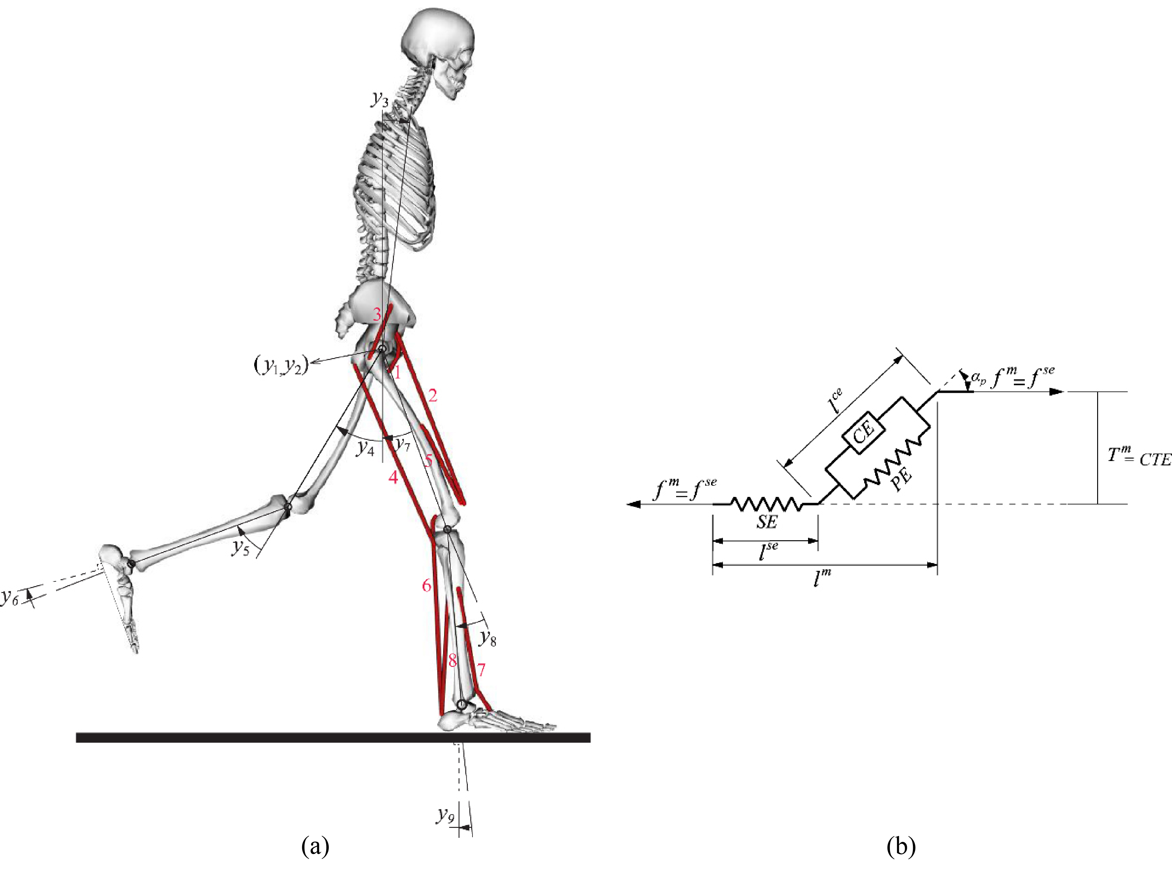$\alpha_{p}$ , the total muscle (musculotendon) length by $l^{m}$ , the SE length by $l^{\textit{se}}$ , the CE length by $l^{\textit{ce}}$ , the muscle force by $f^{m}$ and the muscle thickness by $T^{m}$ , which is constant during contraction.

In this study, both the skeletal and muscular system dynamics are computed in an inverse manner based on a novel method, called unconstrained system dynamics of extended inverse dynamics (USDEID), which was previously introduced by Rahmati et al. [24]. When the optimization process is applied with inverse dynamics, the trajectories of the generalized coordinates and muscle forces are represented by simple mathematical functions [25, 26], where the function coefficients are the optimization parameters. In this study, since the optimization problem should be solved for different average velocities, the computational effort can be prohibitive. Therefore, the USDEID approach was employed to overcome this problem.

The aim of this study is to investigate the effect of average velocities on the prediction of the movement trajectories in the SSP, and whether the predictive gait simulation is able to estimate the realistic alterations of joint angles, the positions of the hip and ankle joints corresponding to the swing leg, and the muscle activations for the different gait average velocities, ranging from normal to fast. At first, the predictive gait simulation was validated for the SSP with normal average velocity by comparison of the optimal and experimental joint angles, GRFs, and muscle activations. Then the validated predictive model was employed to estimate gait motion trajectories, GRFs, and muscle activations for the different average velocities by scaling the time duration of the movement.

2. Materials and methods

Two dynamic systems – muscular, and skeletal – were used to model the human gait. These two systems are coupled via two well-known ordinary differential equations of contraction dynamics, and equations of motion, respectively. Since an inverse approach was used in this study, the muscle activations were estimated from measured gait kinematics as well as muscular forces as input signals by contraction dynamics. The net joint torques produced by the equations of motion corresponding to the skeletal system and the muscle forces should be the same. This relationship is known as the system dynamics, and usually satisfied by an equality constraint in the optimization process for the inverse approaches; however, since the USDEID method was applied here, the compatibility between the skeletal and muscular torques is satisfied by reformulation of the system dynamics [24]. In the optimization procedure, the muscle forces and generalized coordinates were considered as optimization variables, and the cost function of muscle fatigue was minimized subject to the motion constraints for the method of USDEID.

2.1 Skeletal system dynamics

In order to model the skeletal system composed of bones and joint connections, the method of multibody systems is applied here. Indeed, this method is adequate to describe the dynamic behavior of mechanical systems which undergo large, nonlinear motions [27], as occurring during walking. A recursive Newton-Euler formulation is applied to derive the equations of motion for skeletal system in the sagittal plane with seven segments, including right and left feet, shanks, thighs, and HAT (head, arms, trunk) and nine degrees of freedom. The skeletal system is actuated by the net joint torques produced by sixteen muscle groups (Fig. 1a).

The equations of motion are presented as follows:

$\displaystyle\mathbf{M}(\mathbf{y})\ddot{\mathbf{y}}+\mathbf{C}(\mathbf{y},% \dot{\mathbf{y}})+\mathbf{G}(\mathbf{y})-\mathbf{\tau}^{\textit{GRF}}=\mathbf{% R}(\mathbf{y})\mathbf{f}^{m}$ (1)

where $\mathbf{y}=[y_{1}\>y_{2}\>\ldots\>y_{9}]^{T}$ is the vector of generalized coordinates corresponding to the number of degrees of freedom of the skeletal system, $\mathbf{M}(\mathbf{y})$ is the symmetric, positive definite 9 $\times$ 9 – mass matrix, $\mathbf{C}(\mathbf{y},\dot{\mathbf{y}})$ is the 9 $\times$ 1 – vector of generalized centrifugal and Coriolis forces, $\mathbf{G}(\mathbf{y})$ is the 9 $\times$ 1 – vector of generalized gravitational forces, $\mathbf{\tau}^{\textit{GRF}}$ is the 9 $\times$ 1 – vector of generalized applied forces of the GRF, $\mathbf{R}(\mathbf{y})$ is the 9 $\times$ 16 matrix that transforms the muscle forces into generalized forces; and $\mathbf{f}^{m}$ is the 16 $\times$ 1 vector of muscle forces. The GRF is considered as a vector exerted on a specific point of stance foot at each moment of time during the SSP. It’s value, direction and application point can be computed by the equations of motion based on $\mathbf{y}$ , $\dot{\mathbf{y}}$ , and $\ddot{\mathbf{y}}$ .

2.2 Muscular dynamics

Muscles are the actuators of the musculoskeletal control system [28] and basically consist of three elements: (a) a contractile element (CE) simulating muscle fibers which produce force, (b) a non-linear series elastic (SE) element representing tendons which are in series with the CE, and (c) connective tissues which are parallel to the CE and operate as a non-linear parallel elastic (PE) element. The motion about the joint is generated by the torque applied by the moment arm corresponding to muscle force. In order to compute the muscle forces, the muscle lengths should be first estimated. The muscle lengths can be calculated as functions of the generalized coordinates by the expressions or tables available in the literature [29]. In this study, the muscle lengths were specified based on the following expression proposed by Gerritsen et al. [30]:

$\displaystyle l^{m}=l_{0}^{m}+r_{a}\left(\frac{\pi}{2}-\gamma\right)+r_{k}% \beta-r_{h}\alpha$ (2)

where $\alpha$ , $\beta$ , and $\gamma$ are the angles between thigh and HAT, shank and thigh, and foot and shank, respectively; furthermore, the parameters $r_{a}$ , $r_{k}$ , and $l_{0}^{m}$ represent the moment arms about the ankle, knee, and hip joints and muscle length at full extension of the joints, respectively. These parameters are listed in the Appendix of Ackermann [23] (available in the table of muscle parameters). By differentiating Eq. (2) with respect to time, shortening/lengthening velocity of the muscle can be computed.

A model for muscle contraction dynamics was presented by Hill [31]. A review of these models is given by Winters [32]. According to the three-element Hill-type muscle model, the muscle force is determined as a function of muscle activation level ( $a$ ), passive characteristics of the PE, and force generation characteristics specified by force-length and force-velocity relations of the CE. A three-element Hill-type model of a skeletal muscle is shown in Fig. 1b. The total muscle force is computed based on the muscle model presented in Fig. 1b; force generation; and passive characteristics (see Appendix).

Figure 2.

Foot-ground contact model for: (a) foot flat and midstance phases, and (b) heel-off phase. Rh, Rvh, and Rvm are horizontal reaction force, vertical reaction forces on the contact points of heel and metatarsophalangeal joints, respectively.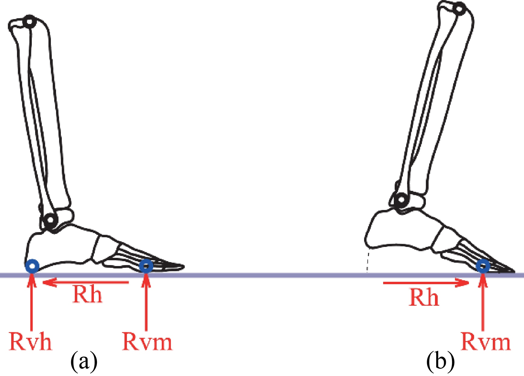

Figure 3.

Optimization procedure for trajectory prediction in SSP.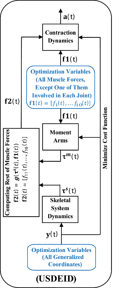

2.3 Foot-ground contact model

A two-point foot contact model was employed in this study [23]. In SSP, the stance foot passes through three main phases, including loading response, mid-stance, and terminal stance, which are in accordance with foot flat, mid-stance, and heel-off, respectively. From a biomechanical perspective, foot-ground contact can be simply modelled by the heel and metatarsal contact points. In foot flat and mid-stance phases, both contact points of the heel and metatarsal are in touch with the ground, while in heel-off phase only metatarsal is in touch with the ground, as shown in Fig. 2.

The GRFs, applied on the contact points in the vertical direction should be unilateral and positive to ensure that the contact points push the ground. The negative values mean the stance foot stuck to the ground, which is not acceptable during the gait cycle. However, it is adequate to formulate them as bilateral constraints and impose constraints to the optimization process that ensure positive vertical reaction forces. Similarly, the horizontal GRFs can be formulated generally, and then in the optimization process their magnitudes are limited to avoid sliding by satisfying the Coulomb’s friction law.

2.4 Optimization procedure

There are different optimization procedures for biomechanical analysis of human movement in the literature: (a) static optimization [33, 34], which is computationally efficient, but requires the use of an instantaneous cost function, leading often to unrealistic estimations of muscle forces [23], and (b) dynamic optimization [35] based on the parameterization of the motion using Fourier series [36], splines of class C ${}^{3}$ [37] or splines of class C ${}^{2}$ [9], which is computationally very costly. Since more realistic estimation of muscle forces can be obtained by the integration of the muscle fatigue as the energy expenditure, the so-called dynamic optimization, in opposition to the static optimization that was employed in this study, in conjunction with the approach of USDEID [24]. The optimization procedure of solving problem is shown in Fig. 3. The optimization problem was solved by MATLAB sequential quadratic programming (SQP) toolbox with enabled option of parallel computing. A 4-core machine was used to implement the optimization process.

While a parametric Fourier series was applied to estimate each generalized coordinate, a parametric square Fourier series was employed to compute each muscle force during the SSP. The positive values of square Fourier series guarantee the force contraction behavior of the muscles in one direction. The parametric functions are presented by Eq. (3) as follows:

$\displaystyle\left\{\begin{array}[]{lc}y_{i}(t)=p_{i,0}+\sum\limits_{j=1}^{3}p% _{i,j}\cos(j\times\omega_{i}\times t)+\sum\limits_{j=1}^{3}q_{i,j}\sin(j\times% \omega_{i}\times t),&i=1,\ldots,9\\ f_{k}^{m}(t)=\left(p_{k,0}+\sum\limits_{j=1}^{3}p_{k,j}\cos(j\times\omega_{k}% \times t)+\sum\limits_{j=1}^{3}q_{k,j}\sin(j\times\omega_{k}\times t)\right)^{% 2},&k=1,\ldots,10\\ \end{array}\right.$ (3)

Optimal control parameters are the coefficients and frequency of Fourier series in Eq. (3) with the upper and lower bounds of 10 and $-$ 10 for the generalized coordinates, and 60 and $-$ 60 for the muscle forces. These bounds provide the possibility to estimate the high and low values of generalized coordinates and muscle forces, while the search space is decreased considerably, which can prevent high computational cost. The experimental values measured by the motion analysis of normal speed and bounded random values were used as the initial guess for the optimal control parameters of generalized coordinates and muscle forces, respectively. In order to isolate the performance of optimization processes from the initial values, the same initial guess was used for the control parameters of all different speeds.

During the optimization procedure, the values of the generalized coordinates and muscle forces in the USDEID approach were determined by assigning numerical values to the control parameters. Therefore, net skeletal torques were computed by the equations of motion, shown on the left side of Eq. (1) and the net muscular torques by the muscle forces and their moment arms, shown on the right side of Eq. (1). The full compatibility of these two types of torques was provided by the method of USDEID [24]. The number of control nodes devoted to each of the generalized coordinates and muscle forces was set to 24 with time intervals of 0.024 s, 0.018 s, 0.012 s, and 0.009 s for the average velocities of 1.55 m/s, 2.07 m/s, 3.10 m/s, and 4.07 m/s, respectively.

2.4.1 Cost function

In this study, energetics was assessed by the integration of muscle fatigue as the cost function in conjunction with Hill-Type muscle model [38]. Muscle fatigue is characterized by a loss of muscle power that results from a decline in both velocity and force. This cost function was proposed by Crowninshield and Brand [38] as follows:

$\displaystyle J_{s}=\sum\limits_{k=1}^{N}\sum\limits_{i=1}^{16}\left(\frac{f_{% ik}^{m}}{\textit{PCSA}_{i}}\right)^{3}$ (4)

where $f_{ik}^{m}$ is the force, applied by muscle “ $i$ ” at time instant $t_{k}$ ; “ $N$ ” is the last time step number; and $\textit{PCSA}_{i}$ is the physiological cross-sectional area of muscle “ $i$ ”.

Figure 4.

Comparison of the predicted and experimental joint angles for normal velocity (1.55 m/s) in SSP. (a) right ankle angle, (b) right knee angle, (c) right hip angle, (d) left ankle angle, (e) left knee angle, and (f) left hip angle.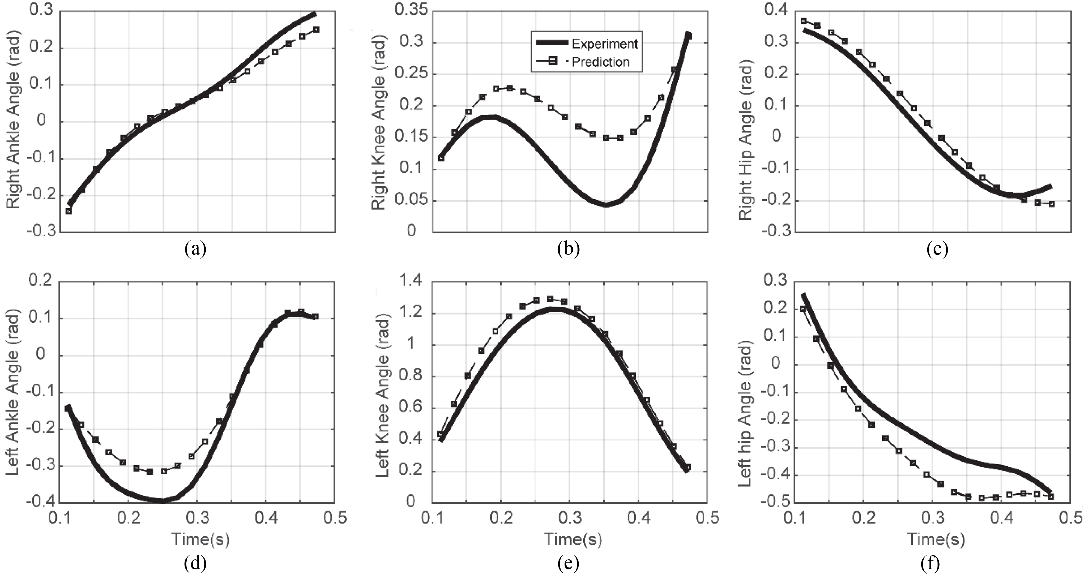

2.4.2 Constraints

Since neuromuscular modelling is defined by normalized activations and an inverse approach was applied; therefore, the estimated activations should be constrained between 0 and 1 for the approach of USDEID, as follows:

$\displaystyle 0\leqslant a_{i}^{m}\leqslant 1,\quad i=1,2,\ldots,16$ (5)

Different types of constraints were employed to predict a valid pattern of walking for SSP. These constraints can be categorized into three types: anatomical constraints which limit the range of motion at joints, the constraints which specify the initial and final body positions of the SSP, and the foot-ground contact constraints. The Eqs (6)–(9) represent the applied optimization constraints as follows:

$\displaystyle y_{i}^{\min}\leqslant y_{i}(t)\leqslant y_{i}^{\max},\quad i=3,% \ldots,9\quad t_{0}\leqslant t\leqslant t_{f}$ (6)

$\displaystyle\left\{\begin{array}[]{l}y_{i}(t_{0})=C_{i}^{0}\quad i=1,\ldots,9% \\ y_{i}(t_{f})=C_{i}^{f}\\ \end{array}\right.$ (7)

$\displaystyle\left\{\begin{array}[]{ll}R_{vh}(t)\geqslant 0&t_{0}\leqslant t% \leqslant t_{f}\\ R_{vm}(t)\geqslant 0&t_{0}\leqslant t\leqslant t_{f}\\ R_{vh}(t)=0&t\geqslant t_{ho}\\ \end{array}\right.$ (8)

$\displaystyle R_{h}(t)\leqslant\mu(R_{vh}(t)+R_{vm}(t))$ (9)

where $C_{i}^{0}$ , $C_{i}^{f}$ , and $t_{ho}$ are the constants, corresponding to the initial and final values of the generalized coordinates, and the moment in which the stance foot heel lifts off the ground, respectively. The coefficient of friction between the foot and the ground is represented by $\mu$ .

The range of motion at joints are limited by Eq. (6). It determines boundary values for the relative angular displacements of the joints. The initial and final conditions for optimization variables are determined by Eq. (7). The foot-ground contact is modelled by Eqs (8) and (9) as optimization constraints. The positive vertical GRFs applied on the heel and metatarsal of stance foot are guaranteed by Eq. (8). It also guarantees the zero values of vertical reaction force at stance foot heel after lifting-off, so the GRFs are only applied on the metatarsal contact point as occurring during SSP after stance foot heel-off. The no-sliding constraint is represented by Eq. (9), in which the horizontal GRF satisfies the Coulomb’s friction law and its magnitude is limited to avoid sliding.

2.5 Experiments

One male healthy subject (32y) free of gait altering injuries participated in this study. Experimental data, including three-dimensional marker positions and GRFs were acquired by the forty-four reflective markers attached on the anatomical locations based on the three-camera VICON Plug-in- Gait marker placement protocol and one Kistler force plate for four normal gait cycle trials with the mean velocity of 1.45 $\pm$ 0.1 m/s. The joint angles were computed by the inverse kinematics from the motion data. The average joint angle and GRF values of these four trials were compared with those estimated by the optimization process, shown in Fig. 3 for the normal average velocity.

The computation of generalized forces requires applying anthropometric data such as segments’ length, mass, center of gravity and moment of inertia. The segments’ length was determined based on marker positions. The other properties were computed based on the table of anthropometric data presented by Winter [1].

The simulated muscle activations were validated against the experimental data taken from Winter [1], which provides muscle EMGs, acquired from several subjects and trials for the normal speed walking.

3. Results and discussion

The results of this study can be divided into two categories: (a) comparison of the experimental and predicted joint angles and GRFs for the normal average velocity and (b) comparison of the predicted joint angles, GRFs, actuating torques, vertical positions of swing leg ankle, knee and hip, COG position, and muscle activations estimated by the approach of USDEID for the different average velocities, ranging from normal (1.55 m/s) to fast (4.07 m/s).

In order to investigate the effect of velocity alterations on the trajectories of the movement by gait prediction, it is necessary first to validate the walking prediction model for the normal velocity. Therefore, the optimization procedure proposed in Fig. 3 was employed to predict the SSP. Figure 4a–f depict the comparison of the predicted and experimental joint angles for normal velocity. The stance and swing feet are the right and left feet, respectively.

A good agreement is observed between the joint angle patterns of simulation results and experiments. It is found that the total mean of squared errors (MSE) is 7% for the all joint angles. The estimated MSE of the joint angles for right and left ankle, knee, and hip are 2.1%, 4.2%, 21.7%, 0.7%, 3.6%, and 9.5%, respectively. Although the MSE values are not negligible, a high compatibility between the simulated and experimental patterns is observed particularly in the case of extremums.

Figure 5.

Comparison of the predicted and experimental GRFs for normal velocity (1.55 m/s) in SSP. (a) horizontal ground reaction force, and (b) vertical ground reaction force.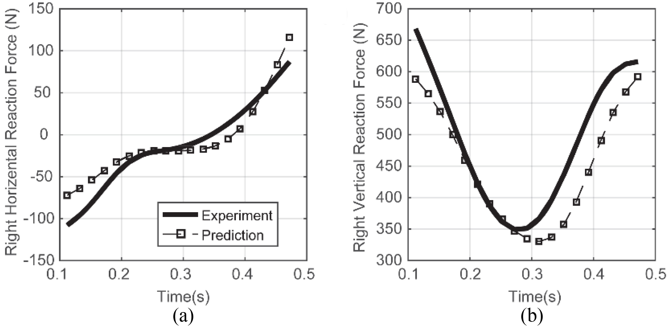

Figure 6.

Comparison of the predicted joint angles for different average velocities, ranging from 1.55 m/s to 4.07 m/s in SSP. (a) right ankle angle, (b) right knee angle, (c) right hip angle, (d) left ankle angle, (e) left knee angle, and (f) left hip angle.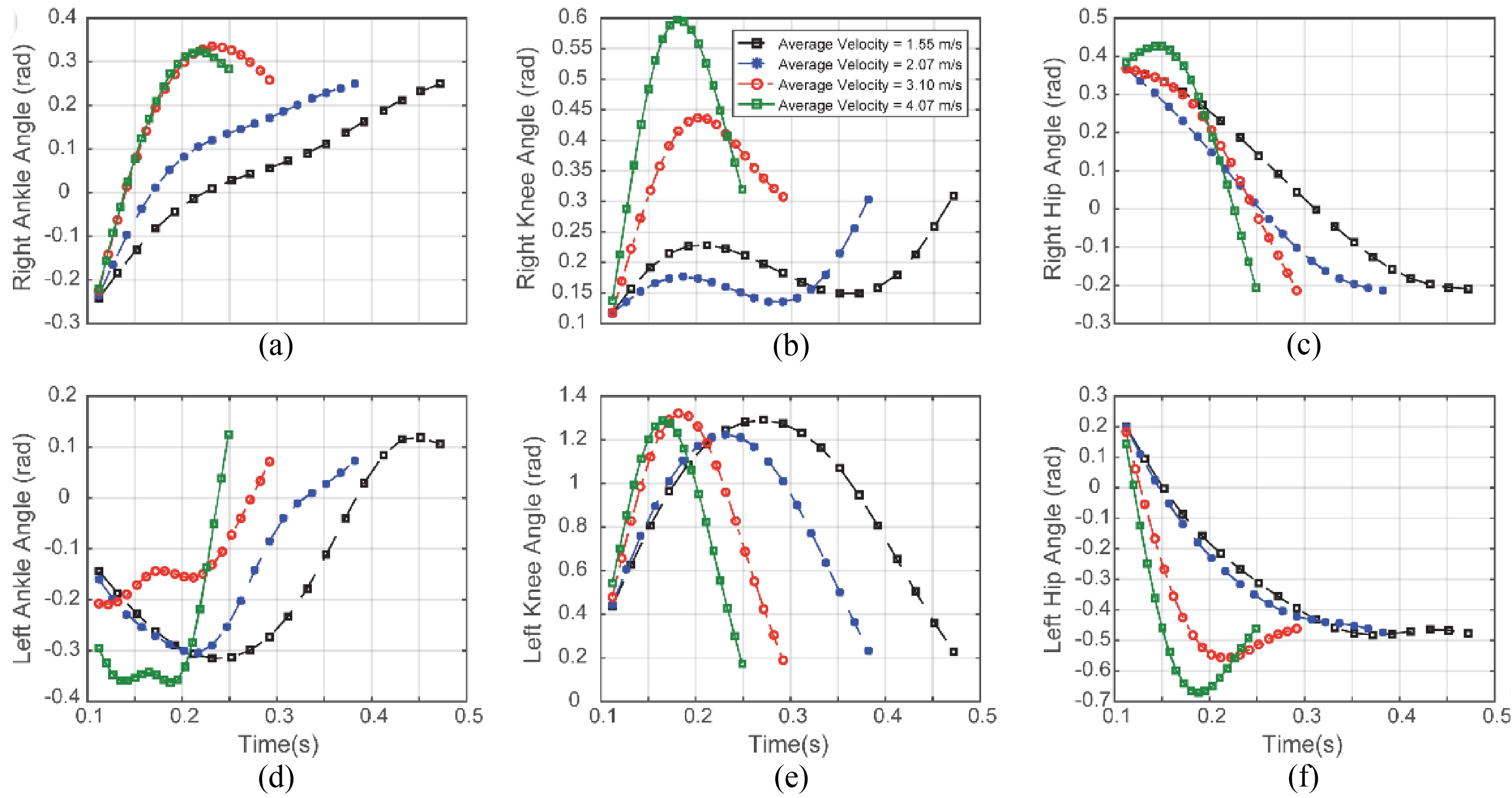

The difference between simulated and experimental results can be addressed to the cost function and the experimental errors such as assumption of ideal revolute joints and marker displacement on the skin. Compared to the simulated joint angles, the experimental results show further alterations particularly in the right knee and left ankle angles (see Fig. 4). This indicates that the gait prediction leads to a more upright movement than the experiment, which is due to the use of integration of the muscle fatigue as cost function. Therefore, as a solution, employing a sthenic criterion which penalize energetics less than the proposed cost function may lead to a more realistic movement. The real joints are composed of complex surface contacts providing moving instantaneous center of rotation between the adjacent limbs and translation. The joints modelled in this study are considered ideal, in which no translation is allowed and their center of rotation is fixed. This assumption, which is essential for multibody system dynamics modelling was justified by Ackermann [23]. For big movements, similar to the ones occurring during gait, the joints can be appropriately modelled as ideal joints that allow no translation and present a fixed center of rotation with acceptable errors [23].

Figure 7.

Comparison of the predicted and experimental GRFs for different average velocities, ranging from 1.55 m/s to 4.07 m/s in SSP. (a) horizental ground reaction force, and (b) vertical ground reaction force.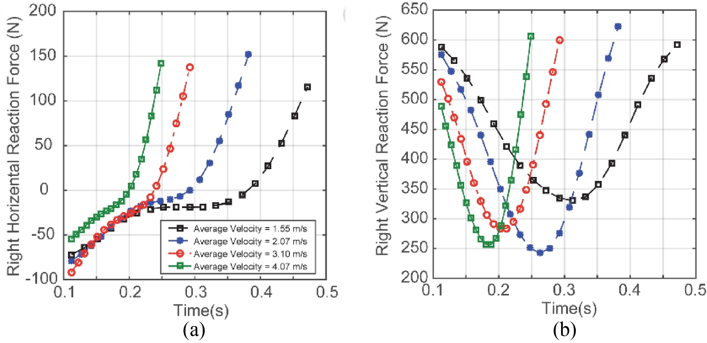

Figure 8.

Comparison of the predicted joint torques for different average velocities, ranging from 1.55 m/s to 4.07 m/s in SSP. (a) right ankle angle, (b) right knee angle, (c) right hip angle, (d) left ankle angle, (e) left knee angle, and (f) left hip angle.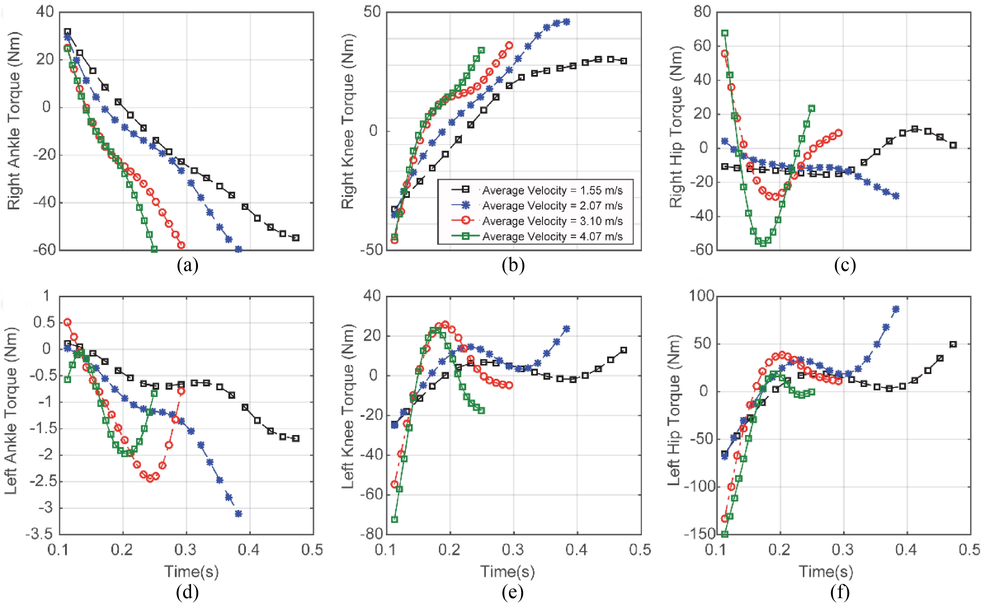

Figure 5 shows the predicted and experimental GRFs. The MSE are 11% and 1% for horizontal and vertical reaction forces, respectively. Similar to joint angles, the predicted GRFs show a good agreement with experimental data. As it is shown by the measured data from the force plate, the values of horizontal reaction force transfer from negative to positive during mid-stance phase, and also a minimum is observed for the vertical reaction force. The simulation results are consistent with these findings.

The simulation results based on optimization procedure for the normal velocity show that the proposed model can be used to predict the SSP at least in term of the movement pattern. Therefore, the validated model can be used to predict the SSP for the different average velocities, ranging from normal to fast.

The comparison of the simulated joint angles for different average velocities is shown in Fig. 6. It is observed that the faster walking leads to further alterations in the joint angle magnitudes, compared to the normal, and also the movement pattern changes for the all joint angles, except left knee. It indicates that the increasing walking speed changes the joint angles in term of both magnitude and pattern.

The GRFs estimated for the different average velocities are shown in Fig. 7. Despite the simulation results of joint angles, the patterns of simulated GRFs are the same for the different speeds. However, considerable changes are observed in their magnitudes. These findings can be compared to the experimental evidences reported by Neptune and Sasaki [39]. These evidences show that in the early mid-stance, there are slight differences for the horizontal reaction forces corresponding to different speeds, however significant differences can be found in the late mid-stance. It is also observed that the vertical reaction force decreases with increasing average velocity during mid-stance [39]. The simulation results are well compatible with these experimental evidences.

The actuating joint torques, shown in Fig. 8 is an important criterion to investigate the biomechanics of gait. They represent the net torques, produced by the muscles. As it is observed, there are differences for the predicted joint torques in both pattern and magnitude during SSP. Each curve shown in Fig. 8 is divided to 19 nodes, so the magnitude of curves can be compared in each similar node. Based on this estimation, it can be observed that generally with increasing average velocity, the corresponding actuating torque increases. The estimated sum of square torques of all joints for the average velocities of 1.55 m/s, 2.07 m/s, 3.10 m/s, and 4.07 m/s are 1645 (Nm ${}^{2}$ ), 2025 (Nm ${}^{2}$ ), 2225 (Nm ${}^{2}$ ), and 2584 (Nm ${}^{2}$ ), respectively.

The mean square torques for the all increased average velocities in the joints of right ankle, knee, hip, and left ankle, knee, hip are 485 Nm ${}^{2}$ , 390 Nm ${}^{2}$ , 392 Nm ${}^{2}$ , 685 Nm ${}^{2}$ , 302 Nm ${}^{2}$ and 23 Nm ${}^{2}$ , respectively, while the square torques for the normal velocity are 520 Nm ${}^{2}$ , 400 Nm ${}^{2}$ , 199 Nm ${}^{2}$ , 391 Nm ${}^{2}$ , 122 Nm ${}^{2}$ and 14 Nm ${}^{2}$ in the right ankle, knee, hip, and left ankle, knee, hip joints, respectively. This finding explains how the actuating joint torques contribute in increasing speed. The comparison between the joint torques of the normal and increased average velocities show that in order to move faster in SSP, the more increased energy expenditure is required in the joints of swing leg and hip joint of the stance leg. It also indicates that not only the energy expenditure does not increase in the ankle and knee joints of the stance leg, but even decreases with increasing velocity.

The maximum energy expenditure among the joint torques for the walking with normal velocity belongs to the ankle of the stance leg, while for the walking with fast velocity belongs to the hip of swing leg. This may be addressed to the more forward movement of the trunk, which occurs during fast walking. In order to keep the balance when the legs move faster and to produce an efficient walking, the trunk should be flexed, so more energy expenditure is required in the hip joint.

Figure 9.

Comparison of the predicted vertical positions for different average velocities, ranging from 1.55 m/s to 4.07 m/s in SSP. (a) left ankle, (b) left knee, (c) left hip, and (d) COG.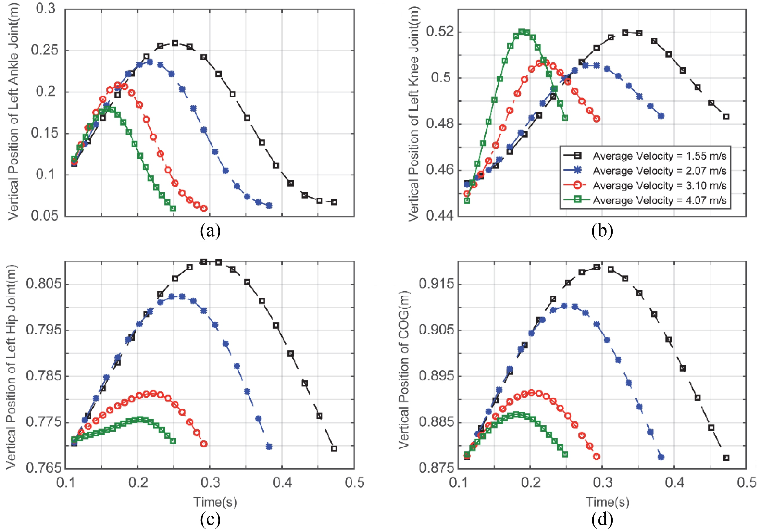

Figure 10.

Comparison of the simulated muscle activations for different average velocities, ranging from 1.55 m/s to 4.07 m/s in SSP. Simulated muscle activations corresponding to the normal velocity (1.55 m/s) are compared against the muscle EMGs (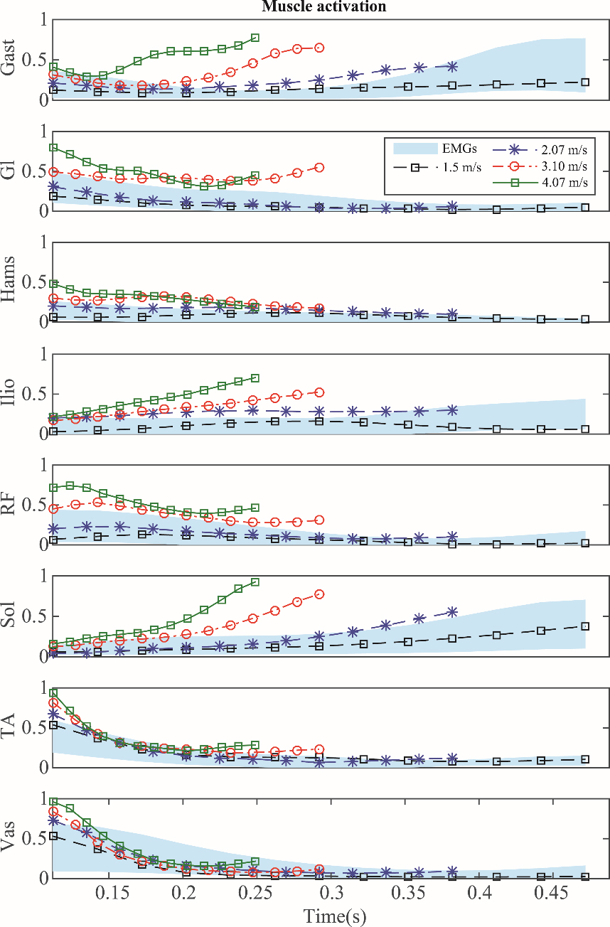 $\mu\pm\sigma$ ), presented by Winter [1].

Figure 11.

Comparison of the schematic views of the predicted normal and fast walking. (a) average velocity is 1.55 m/s, (b) average velocity is 4.07 m/s.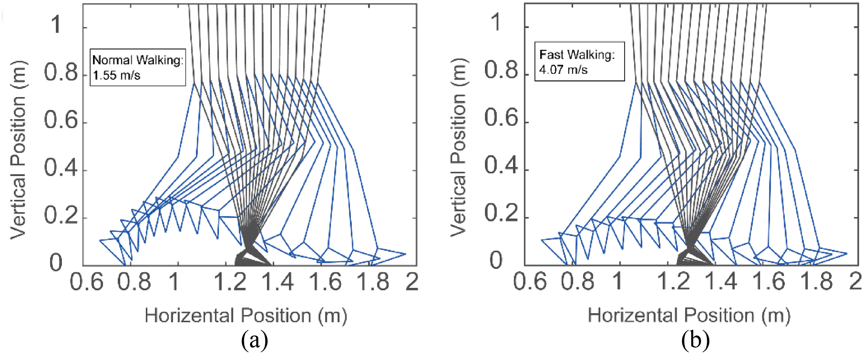

The comparison between experimental and simulated vertical positions of the joints, particularly the ankle and hip joints of the swing leg was employed as a benchmark test to investigate the valid performance of the gait prediction for different speeds. The experimental evidence supports this hypothesis, that the vertical positions of the ankle and hip joints of the swing leg decrease during SSP with increasing average velocities [19]. Figure 9a and c show the same pattern of movement for left ankle and hip joints. A reason for this observation might be seen in the fact that inertial forces associated to the larger accelerations of the segments gets larger than gravitational forces at higher speeds, leading to a less ballistic optimal motion of the lower segments. However, a known pattern of movement for the vertical position of the swing knee has not been found in the literature and in the results of this study.

The vertical COG displacement has been shown to increase with velocity [19, 40], however Fig. 9d does not support this finding. This can be due to modelling the whole upper body with one segment (HAT), which does not allow the realistic alterations of COG. The emphasized upper limb swing decreases the magnitude of vertical oscillations of the body center of gravity [40]. Therefore, if the upper body is modelled by the emphasized upper limb swing, the vertical position of COG may increase with velocity.

The comparison of the muscle activations corresponding to the different average velocities for the eight muscle groups of the right leg during half of a gait cycle is shown in Fig. 10; in addition, the muscle activations estimated for the normal speed are compared against the experimental data (blue shaded area) taken from Winter [1]. Simulated activation results corresponding to the normal speed have satisfied the lower and upper bounds of EMGs within the specified tolerance. The simulated results and EMGs show the same levels of activation for the all muscle groups. This confirms the validity of the optimization process. The comparison of the muscle activations corresponding to the normal speed with those of increased speeds show that with enhancing average velocity, the muscle activations increase, especially for the muscle groups of gastrocnemius, glutei, iliopsoas, rectus femoris, and soleus. It is also observed that, although the activation patterns corresponding to the different speeds are the same for the muscle groups of hamstrings, rectus femoris, soleus, tibialis anterior, and vasti, the activations of gastrocnemius, glutei, and iliopsoas show different patterns with increasing velocity. In these three muscle groups, an enhanced level of activation is observed during the terminal stance for the increased speeds, despite the low level of activation for the normal speed.

To have a better perspective of the alterations in the gait trajectory caused by increasing speed, the schematic views of the movement are shown in Fig. 11a and b for the average velocities of 1.55 m/s and 4.07 m/s, respectively. The reduction in the vertical position of left ankle corresponding to the swing leg is obvious. A more flexion of the HAT is observed for the fast walking in comparison to the normal walking. This finding is compatible with the experimental evidence explains the flexion of the upper body during running. Although the alterations of the speed effect on the joint angle patterns (see Fig. 6), a same sinusoidal pattern is observed for the positions of the hip and left ankle joints in the sagittal plane.

4. Conclusion

This study dealt with the trajectory prediction of the SSP for the average velocities, ranging from normal to fast. The alterations of movement kinematics and kinetics including joint angles, GRFs, joint positions, COG position, joint torques, and muscle activations were investigated. A good compatibility was observed between the simulation results and experimental evidences, except for the COG position, which was in contrast to the experiment. The lack of considering the upper body as a multi-segment system was introduced as the possible reason for incorrectly predicted COG position. In order to estimate a better prediction for the gait analysis, the proposed model should be developed, such that the upper body modelled with the upper limb swing. Therefore, the variables such as COG can be assessed more precisely. Since walking is a movement occurring predominantly in the sagittal plane, a two-dimensional model was employed. However, the aspects of walking can be better estimated by three-dimensional models, especially in the frontal plane. Because of the high computational cost of optimization process, the gait prediction was only assessed in the SSP, which is one of the limitation of this study. A complete understanding of speed effect on the gait trajectories requires a complete analysis of gait cycle.

The results of this study suggest that the gait prediction is a strong tool to investigate the gait alterations corresponding to the changes in the average velocity. If the alterations are divided into two categories, including pattern and magnitude, the joint angles and muscle activations show the changes in both categories, however the GRFs and joint positions demonstrate different magnitudes but a same pattern for different walking speeds.

Footnotes

Acknowledgments

The authors would like to thank Laboratory Djavad Mowafaghian Research Center of Intelligent Neuro-Rehabilitation Technologies for assistance regarding gait analysis data.

Conflict of interest

The authors have no conflict of interest to report.

Appendix

The relation between force and velocity for a muscle CE in a concentric contraction with $v^{\textit{ce}}\leqslant 0$ is expressed as [41]:

(A.1) $\displaystyle\frac{f^{\textit{ce}}}{f_{\max}^{m}}=\left[\frac{B_{r}\left(f_{% \textit{isom}}^{\textit{ce}}+A_{r}\right)}{B_{r}-\frac{\bar{v}^{\textit{ce}}}{% f_{\textit{ac}}}}-A_{r}\right]$

where $\bar{v}^{\textit{ce}}=v^{\textit{ce}}/l_{\textit{opt}}^{\textit{ce}}$ , $A_{r}=$ 0.41, $B_{r}=$ 5.2, $l_{\textit{opt}}^{\textit{ce}}$ is the optimal length of muscle fibers, which is listed in the Appendix of Ackermann [23] (available in the table of muscle parameters) for each of the muscle groups, $f_{\max}^{m}$ is the maximum isometric force generated by a muscle group, the parameter $f_{\textit{ac}}$ is defined by $f_{\textit{ac}}=\min(1,3.33\times a)$ [41]. In the present study the value of $f_{\textit{ac}}$ is chosen to be 1 in order to reduce the computational cost. $f_{\textit{isom}}^{\textit{ce}}$ is the muscle isometric force relative to the maximal muscle force $f_{\max}^{m}$ . This variable represents the force-length relation for the CE, which can be modelled by a parabola where the maximum CE force occurs at the optimal fiber length [42] or a Gaussian function. The active force-length relation is represented by a Gaussian function [32]:

(A.2) $\displaystyle f_{\textit{isom}}^{\textit{ce}}=e^{-\left(\bar{l}^{\textit{ce}}-% 1\right)^{2}/\gamma}$

where $\bar{l}^{\textit{ce}}=l^{\textit{ce}}/l^{\textit{ce}}_{\textit{opt}}$ is the normalized muscle fiber length, and $\gamma$ is a shape factor. The value of $\gamma$ was determined as 0.45, which approximates the force-length relationship of individual sarcomeres [42].

The force-velocity relation in an eccentric contraction with $v^{\textit{ce}}>0$ is expressed as [43]:

(A.3) $\displaystyle\frac{f^{\textit{ce}}}{f_{\max}^{m}}=\left[\frac{b_{1}}{b_{3}-% \bar{v}^{\textit{ce}}}-b_{2}\right]$

where:

(A.4) $\displaystyle b_{1}=\frac{f_{\textit{ac}}B_{r}\left(f_{\textit{isom}}^{\textit% {ce}}+b_{2}\right)^{2}}{\left(f_{\textit{isom}}^{\textit{ce}}+A_{r}\right)% \textit{slopefactor}}$ (A.5) $\displaystyle b_{2}=-f_{\textit{isom}}^{\textit{ce}}f_{\textit{asympt}}$ (A.6) $\displaystyle b_{3}=\frac{b_{1}}{f_{\textit{isom}}^{\textit{ce}}+b_{2}}$

and slopefactor is the ratio of the eccentric derivative of the muscle CE force-velocity curve $(df^{\textit{ce}}/dv^{\textit{ce}})_{\textit{eccentric}}$ to the concentric derivative of the muscle CE force-velocity curve $(df^{\textit{ce}}/dv^{\textit{ce}})_{\textit{concentric}}$ at $v^{\textit{ce}}=0$ . A slopefactor $=$ 2 was adopted by van Soest and Bobbert [41]; however, in the present study a slopefactor $=$ 1 is used to avoid discontinuities, as suggested by Ackermann [23]. $f_{\textit{asympt}}$ is the asymptotic maximum force value of the muscle CE force-velocity curve, considered 1.5 by van Soest and Bobbert [41].

The force generated by the muscle PE can be expressed as [44]:

(A.7) $\displaystyle\frac{f^{\textit{pe}}}{f_{\max}^{m}}=\frac{e^{k^{\textit{PE}}% \left(\bar{l}^{\textit{ce}}-1\right)/\varepsilon_{0}^{\textit{ce}}}-1}{e^{k^{% \textit{PE}}}-1}$

where $k^{\textit{PE}}$ is an exponential shape factor, and $\varepsilon_{0}^{\textit{ce}}$ is the passive muscle strain due to maximum isometric force. The value of shape factor, $k^{\textit{PE}}$ , is set equal to 5, while $\varepsilon_{0}^{\textit{ce}}$ is set equal to 0.6 [44]. The passive tissue of the muscle (PE) generates force only when the length of CE is greater than the optimal length of CE.

Tendon is modelled by a nonlinear force-strain curve characterized exponentially during an initial toe region and linearly thereafter [44], as follows:

(A.8) $\displaystyle\frac{f^{\textit{se}}}{f_{\max}^{m}}=\left\{\begin{array}[]{ll}% \frac{\bar{f}_{\textit{toe}}^{\textit{se}}}{e^{k_{\textit{toe}}}-1}\left(e^{k_% {\textit{toe}}\varepsilon^{\textit{se}}/\varepsilon^{\textit{se}}_{\textit{toe% }}}-1\right);&\varepsilon^{\textit{se}}\leqslant\varepsilon^{\textit{se}}_{% \textit{toe}}\\ k_{\textit{lin}}\left(\varepsilon^{\textit{se}}-\varepsilon^{\textit{se}}_{% \textit{toe}}\right)+\bar{f}_{\textit{toe}}^{\textit{se}};&\varepsilon^{% \textit{se}}>\varepsilon_{\textit{toe}}^{\textit{se}}\\ \end{array}\right.$

where $\varepsilon^{\textit{se}}$ is the tendon strain, $\varepsilon_{\textit{toe}}^{\textit{se}}$ is the tendon strain at initial point of the linear behavior, $k_{\textit{lin}}$ is a linear scale factor, $k_{\textit{toe}}$ is an exponential shape factor, which is set equal to 3 [44], $\bar{f}_{\textit{toe}}^{\textit{se}}$ is the tendon force normalized to maximum isometric force at the initial point, which the tendon exhibits linear behavior. Tendon strain, $\varepsilon^{\textit{se}}$ is characterized by $\varepsilon^{\textit{se}}=(l^{\textit{se}}-l_{\textit{slack}})/l_{\textit{% slack}}$ , where $l_{\textit{slack}}$ is the tendon slack length, at which the tendon or SE starts to transfer force. For the tendon lengths shorter than the slack length, no force is transferred to the skeletal system. For the normalized tendon forces greater than $\bar{f}_{\textit{toe}}^{\textit{se}}=$ 0.33, the transition from nonlinear to linear behavior occurs [45]. The values of $\varepsilon_{\textit{toe}}^{\textit{se}}=0.609\varepsilon_{0}^{\textit{se}}$ and $k_{\textit{lin}}=1.712/\varepsilon_{0}^{\textit{se}}$ , characterized by a strain $\varepsilon_{0}^{\textit{se}}$ of 4% occurring at the maximal isometric muscle force [32], are required for the continuity of slopes at the transition.

To obtain the whole force generated by active part of the muscle, the muscle CE force should be scaled by the activation level ( $a$ ). Therefore, the total muscle force can be estimated, as shown in Fig. 1b, by the sum of the PE and scaled CE forces, and multiplying it by $\cos(\alpha_{p})$ , as follows:

(A.9) $\displaystyle f^{m}=\left(f^{\textit{ce}}\times a+f^{\textit{pe}}\right)\cos(% \alpha_{p})$

The only variables that can be computed directly from the skeletal system are generalized coordinates and their derivatives, which can be used to estimate total muscle length and shortening/lengthening velocity. In order to apply Eq. (A.9) for inverse dynamics approaches, it should be rewritten based on muscle length according to Fig. 1b, shortening/lengthening velocity, and activation.

References

Winter

. Biomechanics and motor control of human gait: Normal, elderly and pathological. 1991.

Kim

Abdel-Malek

Xiang

Yang

Arora

. Concurrent motion planning and reaction load distribution for redundant dynamic systems under external holonomic constraints. International Journal for Numerical Methods in Engineering 2011; 88(1): 47-65.

Golliday

Hemami

. An approach to analyzing biped locomotion dynamics and designing robot locomotion controls. IEEE Transactions on Automatic Control 1977; 22(6): 963-72.

Kuo

. The six determinants of gait and the inverted pendulum analogy: A dynamic walking perspective. Human Movement Science 2007; 26(4): 617-56.

Anderson

Pandy

. Dynamic optimization of human walking. Journal of Biomechanical Engineering 2001; 123(5): 381-90.

Langenderfer

LaScalza

Mell

Carpenter

Kuhn

Hughes

. An EMG-driven model of the upper extremity and estimation of long head biceps force. Computers in Biology and Medicine 2005; 35(1): 25-39.

Allouch

Boudaoud

Younès

Ben-Mansour

Marin

. Proposition, identification, and experimental evaluation of an inverse dynamic neuromusculoskeletal model for the human finger. Computers in Biology and Medicine 2015; 63: 64-73.

Xie

Zhang

. A patient-specific EMG-driven neuromuscular model for the potential use of human-inspired gait rehabilitation robots. Computers in Biology and Medicine 2016; 70: 88-98.

Saidouni

Bessonnet

. Generating globally optimised sagittal gait cycles of a biped robot. Robotica 2003; 21(02): 199-210.

10.

Shourijeh

McPhee

. Forward dynamic optimization of human gait simulations: A global parameterization approach. Journal of Computational and Nonlinear Dynamics 2014; 9(3): 031018.

11.

Martin

Schmiedeler

. Predicting human walking gaits with a simple planar model. Journal of Biomechanics 2014; 47(6): 1416-21.

12.

Chevallereau

Bessonnet

Abba

Aoustin

. Bipedal robots: Modeling, design and walking synthesis. John Wiley and Sons; 2013.

13.

van den Ackermann

Bogert

. Optimality principles for model-based prediction of human gait. Journal of Biomechanics 2010; 43(6): 1055-60.

14.

Ren

Jones

Howard

. Predictive modelling of human walking over a complete gait cycle. Journal of Biomechanics 2007; 40(7): 1567-74.

15.

Xiang

Arora

Abdel-Malek

. Optimization-based prediction of asymmetric human gait. Journal of Biomechanics 2011; 44(4): 683-93.

16.

Kirtley

Whittle

Jefferson

. Influence of walking speed on gait parameters. Journal of Biomedical Engineering 1985; 7(4): 282-8.

17.

Lythgo

Wilson

Galea

. Basic gait and symmetry measures for primary school-aged children and young adults. II: Walking at slow, free and fast speed. Gait and Posture 2011; 33(1): 29-35.

18.

Oberg

Karsznia

Oberg

. Joint angle parameters in gait: Reference data for normal subjects, 10–79 years of age. Journal of rehabilitation Research and Development 1994; 31(3): 199-213.

19.

Zhao

Zhang

Wang

, editors. Three-dimensional motion of the pelvis during human walking. Mechatronics and Automation, 2005 IEEE International Conference 2005; IEEE.

20.

Zajac

Winters

. Modeling musculoskeletal movement systems: Joint and body segmental dynamics, musculoskeletal actuation, and neuromuscular control. Multiple Muscle Systems. Springer; 1990; 121-48.

21.

Pandy

. Computer modeling and simulation of human movement. Annual Review of Biomedical Engineering 2001; 3(1): 245-73.

22.

Marshall

Wood

Jennings

. Performance objectives in human movement: A review and application to the stance phase of normal walking. Human Movement Science 1989; 8(6): 571-94.

23.

Ackermann

. Dynamics and energetics of walking with prostheses. University of Stuttgart; 2007.

24.

Rahmati

Rostami

Beigzadeh

. A low-cost optimization framework to solve muscle redundancy problem. Nonlinear Dynamics 2017; 1-15.

25.

Yen

Nagurka

. Suboptimal trajectory planning of a five-link human locomotion model. Biomechanics of Normal and Prosthetic Gait 1987; 4: 17-22.

26.

Koopman

Grootenboer

De Jongh

. An inverse dynamics model for the analysis, reconstruction and prediction of bipedal walking. Journal of Biomechanics 1995; 28(11): 1369-76.

27.

Schiehlen

. Multibody system dynamics: Roots and perspectives. Multibody System Dynamics 1997; 1(2): 149-88.

28.

Vilimek

. Musculotendon forces derived by different muscle models. Acta of Bioengineering and Biomechanics 2007; 9(2): 41.

29.

Menegaldo

de Toledo Fleury

Weber

. Moment arms and musculotendon lengths estimation for a three-dimensional lower-limb model. Journal of Biomechanics 2004; 37(9): 1447-53.

30.

Gerritsen

van den Bogert

Hulliger

Zernicke

. Intrinsic muscle properties facilitate locomotor control – a computer simulation study. Motor Control 1998; 2(3): 206-20.

31.

Hill

. The heat of shortening and the dynamic constants of muscle. Proceedings of the Royal Society of London B: Biological Sciences 1938; 126(843): 136-95.

32.

Winters

. Hill-based muscle models: A systems engineering perspective. Multiple Muscle Systems. Springer; 1990; 69-93.

33.

Heintz

Gutierrez-Farewik

. Static optimization of muscle forces during gait in comparison to EMG-to-force processing approach. Gait and Posture 2007; 26(2): 279-88.

34.

Raikova

Aladjov

. Hierarchical genetic algorithm versus static optimization – investigation of elbow flexion and extension movements. Journal of Biomechanics 2002; 35(8): 1123-35.

35.

Pelta

Cruz

Verdegay

. Simple control rules in a cooperative system for dynamic optimisation problems. International Journal of General Systems 2009; 38(7): 701-17.

36.

Peasgood

Kubica

McPhee

. Stabilization of a dynamic walking gait simulation. Journal of Computational And Nonlinear Dynamics 2007; 2(1): 65-72.

37.

Bessonnet

Seguin

Sardain

. A parametric optimization approach to walking pattern synthesis. The International Journal of Robotics Research 2005; 24(7): 523-36.

38.

Crowninshield

Brand

. A physiologically based criterion of muscle force prediction in locomotion. Journal of Biomechanics 1981; 14(11): 793-801.

39.

Neptune

Sasaki

. Ankle plantar flexor force production is an important determinant of the preferred walk-to-run transition speed. Journal of Experimental Biology 2005; 208(5): 799-808.

40.

Lulić

Sušić

Kodvanj

. Biomechanical analysis of walking: Effects of gait velocity and arm swing amplitude. Periodicum Biologorum 2010; 112(1): 13-7.

41.

van Soest

Bobbert

. The contribution of muscle properties in the control of explosive movements. Biological Cybernetics 1993; 69(3): 195-204.

42.

Gordon

Huxley

Julian

. The variation in isometric tension with sarcomere length in vertebrate muscle fibres. The Journal of Physiology 1966; 184(1): 170-92.

43.

Cole

van den Bogert

Herzog

Gerritsen

. Modelling of force production in skeletal muscle undergoing stretch. Journal of Biomechanics 1996; 29(8): 1091-104.

44.

Thelen

. Adjustment of muscle mechanics model parameters to simulate dynamic contractions in older adults. Transactions-American Society of Mechanical Engineers Journal of Biomechanical Engineering 2003; 125(1): 70-7.

45.

Proske

Morgan

. Tendon stiffness: Methods of measurement and significance for the control of movement. A review. Journal of Biomechanics 1987; 20(1): 75-82.