Intelligent medical image feature extraction method based on improved deep learning

Abstract

BACKGROUND:

Medical patients can be diagnosed early, however it is difficult to extract effective features in medical image segmentation based on semantic information.

OBJECTIVE:

A deep learning based image pixel block feature learning technology is studied in this paper.

METHODS:

The unlabeled image block sample training stack noise reduction automatic encoder is used to learn and extract the deep features of the image, and construct the initial depth neural network model. The labeled samples are used to fine-tune the initial depth neural network model, the deep features of the image correspond to the category, and the depth neural network model with classification function is obtained. The model is used to classify the pixel block samples in the segmented image and detect the initial segmentation region of brain tumor tissue. Finally, threshold segmentation and morphological methods are used to optimize the initial results to obtain accurate segmentation results of brain tumor tissue.

RESULTS:

The results show that this method can effectively improve the accuracy and sensitivity of segmentation. The running speed is also greatly improved compared with the traditional machine learning method.

Keywords

Deep learning intelligent medical image feature extraction method

1. Introduction

Image segmentation is an essential key link in medical image processing and medical image analysis. It is widely used in the pre-processing to peel off the equipment projection, skull and other unrelated tissues, or in the later analysis to extract different organs, tissues and pathological structures, and directly affects the results of subsequent processing and analysis tasks [1].

Convolutional neural network (CNN) is a representative algorithm of supervised learning. Since Hinton et al. proposed the AlexNet network to win the ILSVRC image classification competition in 2012, deep learning has become a hot research topic. CNN is composed of input layer, convolution layer, activation function, pooling layer and full connection layer [2]. Convolution neural network uses the convolution layer and pooling layer to automatically learn image features of various scales. Firstly, it understands image color and brightness, then local information such as edge and line, then texture, shape and other more complex structural information, and finally high-level semantic information of the whole image.

Some scholars use particle swarm optimization convolution kernel (PSO-ConvK) to identify lung tumor images [3]. The random initialization of convolution kernel and gradient descent method to train CNN are easy to fall into the local minimum value, which is solved to a certain extent. Parameter transfer method is used to construct CNN, convolution kernel is extracted, and particle velocity and position are updated continuously by PSO [4]. The global optimal value is found by initialization convolution kernel, and is then transferred to CNN, and the weight is modified by the gradient descent method. The results show that the recognition rate of PSO optimized convolution kernel is always higher than that of random convolution kernel and Gaussian convolution kernel, and the recognition rate is as high as 92.3%.

From the initial manual segmentation, to the coarse segmentation based on gray threshold, and then to a variety of automatic segmentation methods, researchers have been pursuing more efficient, more accurate and more intelligent segmentation technology [5]. Image segmentation based on semantic information is of great significance in medical image processing. By recognizing the semantic information of different physiological tissues in medical images, more accurate segmentation results can be obtained. It is an important analysis method, especially suitable for the detection of structural brain lesions (such as brain tumor, brain injury, cerebral infarction, etc.) and subsequent qualitative analysis.

Because of the complexity of medical images, the key problem of the segmentation method based on semantic information is how to search and extract the features which can fully describe the semantic information of image or pixel. The proposed deep learning brings a new solution [6]. Using the deep learning framework, we can automatically learn the potential deep features and corresponding categories from the samples, and classify the target by trained neural network, thus solving the problem of feature description difficulty in semantic information segmentation.

In this paper, stack noise reduction automatic encoder is used to construct the depth neural network: firstly, fixed size image block samples are extracted from the preprocessed training image set, and then the initial parameters of each layer network are trained by feature learning of unlabeled image block samples, and then the depth neural network has classification function through further fine-tuning the labeled image block samples. Then, the image block samples in the segmented image are classified, and the central pixel of the image block marked as tumor tissue is mapped to the black-and-white binary image as the initial segmentation result; finally, the accurate segmentation result of tumor tissue in brain MRI image is obtained by optimizing the results by using threshold segmentation method and morphological processing method. Figure 1 shows the technical route of this method [7].

Figure 1.

Medical image segmentation method based on the deep neural network.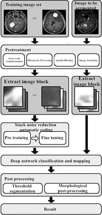

2. Methods

The basic concept of deep learning comes from the early artificial neural network research [8, 9, 10]. The relevant team improved the relevant theory in 2006 and won the Imagenet competition in 2012. After that, it quickly occupied the mainstream research direction in the field of computer vision. In essence, deep learning can be regarded as a feature learning process. By inputting a large number of image data into the deep network and iterating repeatedly, the image features and corresponding categories can be automatically summarized.

In this paper, a deep neural network is constructed by using stacked automatic encoder (SAE) [11]. The model is composed of many layers of automatic encoder (AE) in series. Each layer of automatic encoder is a simple neural network including input layer, intermediate layer and output layer. The principle and implementation method of the automatic encoder and its improved structure are discussed in the next sections.

2.1 Automatic encoder

The standard automatic encoder is a simple neural network with only one intermediate layer, and its structure can be simply summarized into two parts: encoding and decoding [12]. In this process, in order to ensure the integrity of data information, the output results are required to be consistent with the input.

Figure 2 shows the simple structure of an automatic encoder. It can be seen that the automatic encoder is essentially a process of encoding before decoding. Firstly, a large number of unlabeled original data are input, and then the encoder is used to encode the input data to get the dimensionless middle layer data. Then the decoder is used to decode the middle layer data and reconstruct the original data as the output [13]. In this process, if the input data and the output data are completely consistent, the corresponding intermediate data can be regarded as an abstract representation of the original data, that is, the “shallow features” of the original data.

The parameter adjustment process of the automatic encoder is shown in Fig. 3. In order to achieve the purpose that input is output, the parameters of encoder and decoder need to be adjusted continuously according to the error between input data and output data until the error is eliminated.

Figure 2.

Single layer automatic encoder.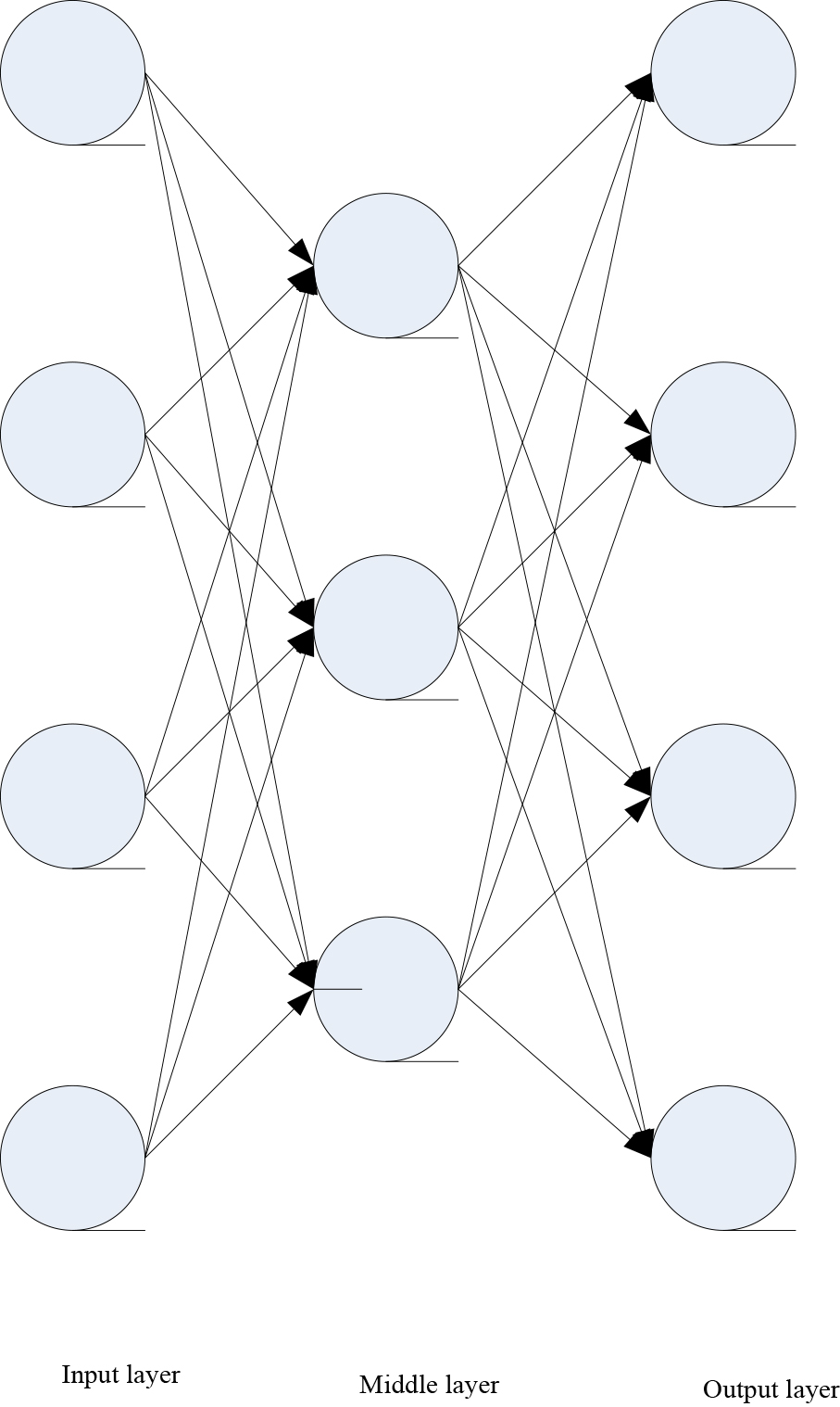

Figure 3.

Single layer automatic encoder.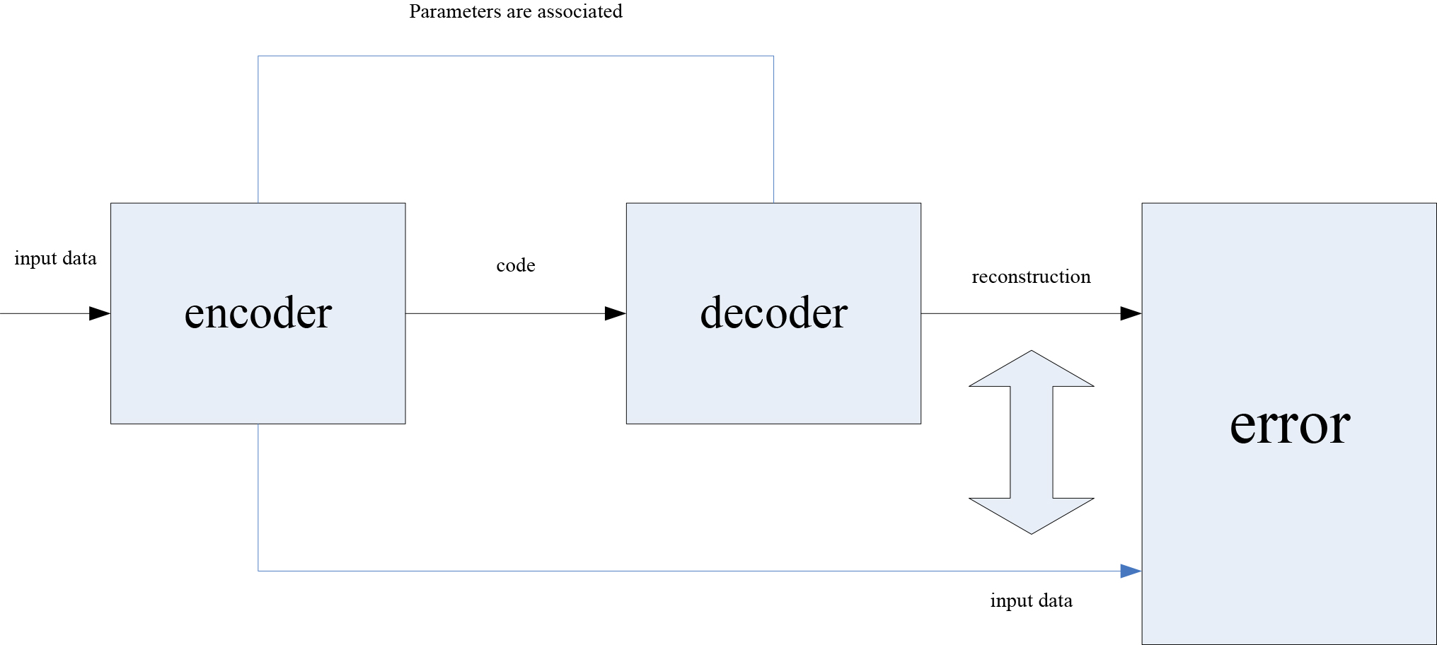

In the specific implementation process, the original data of the input layer is set as $x(x\in[0,1]^{d})$ , and it is mapped to the data $y(y\in[0,1]^{d})$ of the middle layer through the encoder $f$ :

$\displaystyle y=f_{\theta}(x)=\textit{sigm}(Wx+b)$ (1)

Where: sigm refers to the sigmoid activation function, $\theta=\{W,b\}$ is the parameter of encoder $f$ , $W$ is the weight matrix of ${d^{\prime}}\times d$ , and $b$ is the offset.

Then, the decoder $g$ is used to reconstruct the middle layer data $y$ :

$\displaystyle z=g_{\theta^{\prime}}(y)=\textit{sigm}({W^{\prime}}y+{b^{\prime}})$ (2)

Where: ${\theta^{\prime}}=\{{W}^{\prime},{b}^{\prime}\}$ is the parameter of decoder $g$ .

In order to make the input data consistent with the output data, the associated parameters of the encoder and decoder can be adjusted:

$\displaystyle\theta^{*},{\theta^{\prime}}^{*}=\mathop{\arg\min}\limits_{\theta% ,{\theta^{\prime}}}\frac{1}{n}\sum\limits_{i=1}^{n}{L(x_{i}.z_{i})}=\mathop{% \arg\min}\limits_{\theta,{\theta^{\prime}}}\frac{1}{n}\sum\limits_{i=1}^{n}{L(% x_{i}.{g}_{\theta^{\prime}}(f_{\theta}(x_{i})))}$ (3)

The reconstruction error $L$ is calculated as follows:

$\displaystyle L(x,z)=-\sum\limits_{k=1}^{d}{[x_{k}\log z_{k}+(1-x_{k})\log(1-z% _{k})]}$ (4)

When the reconstruction error reaches the minimum, the intermediate data $y$ is considered as the potential representation of the original data $x$ under the premise of lossless information.

2.2 Noise reduction automatic encoder

When using the automatic encoder to extract image features, it is also necessary to optimize the automatic encoder to improve its robustness in processing image data with noise. Some scholars have proposed a noise reduction automatic encoder, as shown in Fig. 4. Its principle is to partially destroy the original data when input, and then let the automatic encoder learn how to reconstruct the original data that has not been damaged before input, so that the generalization ability of the encoder will be enhanced.

Figure 4.

Noise reduction automatic encoder.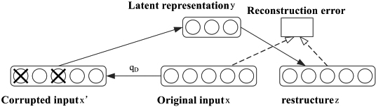

The specific implementation process is as follows: first, the original data $x(x\in[0,1]^{d})$ is transformed into a new input data by adding random noise according to the QD distribution, and then Eqs (1) and (2) are transformed into the following forms:

$\displaystyle y=f_{\theta}(\tilde{x})=\textit{sigm}(W\tilde{x}+b)$ (5) $\displaystyle z=g_{\theta}(y)=\textit{sigm}({W}^{\prime}y+{b}^{\prime})$ (6)

Then, the parameters of encoder and decoder are trained until the reconstruction error $N_{y}$ reaches the minimum:

$\displaystyle\theta^{*},{\theta^{\prime}}^{*}=\mathop{\arg\min}\limits_{\theta% ,{\theta^{\prime}}}\frac{1}{n}\sum\limits_{i=1}^{n}{L(x_{i}.{g}_{\theta^{% \prime}}(f_{\theta}(\tilde{x}_{i})))}$ (7)

It is worth noting that. The biggest difference between the noise reduction automatic encoder and the automatic encoder in the calculation process is that the output data $z$ is obtained from the damaged input data $\tilde{x}$ , rather than the original true value data $x$ . Therefore, the decoder reconstructs the middle layer to obtain the output data approaching to the original data (make $z=x$ ). In this way, the neural network will have a certain degree of noise resistance, and the features extracted from the interlayer are more representative.

The image features extracted by the automatic encoder and noise reduction automatic encoder are shown in Fig. 5. The left picture is the feature block output by the middle layer of the automatic encoder, and it can be seen that the information in the image is relatively messy and difficult to identify; the image on the right is the feature extracted by the automatic noise reduction encoder, which obviously contains more useful information.

Figure 5.

Comparison of the feature extraction of the automatic encoder and noise reduction automatic encoder. a. The characteristics of the output of the intermediate layer of the automatic encoder; b. The characteristics of the output of the intermediate layer of the noise reduction automatic encoder.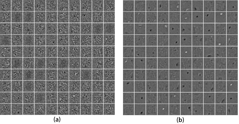

2.3 Image segmentation based on depth neural network

After getting the classification result of each pixel in brain MRI image, the image can be segmented accordingly. In order to eliminate the noise and edge error, the initial segmentation results need to be optimized. In this chapter, the expansion and corrosion of morphological methods are used to obtain more accurate segmentation results.

A stack noise reduction automatic encoder with depth structure can be obtained by connecting several layers of noise reduction automatic encoders in series. The specific method refers to the unsupervised greedy layer by layer training mechanism proposed by scholars, that is, only one automatic encoder is trained at a time, and the middle layer of each layer of automatic encoder is used as the input of the next layer until each layer of automatic encoder is obtained.

First, the original sample data is generated. The final purpose of constructing the deep neural network in this paper is to classify the image pixels, and then use the classification results to achieve tumor tissue segmentation in brain MRI images. Considering the adjacent relationship of similar pixels in the segmentation task, an image block with 25 $\times$ 25 target pixels as the center is used as the sample to be tested, and the category of its central pixel is determined according to the classification results of the image block. In order to standardize the data and eliminate the dimensional influence, it is necessary to normalize the image block, and limit the gray value range of the image block between 0 and 1, as shown in Eq. (8):

$\displaystyle{a}^{\prime}=\frac{a-\min}{\max-\min}$ (8)

Where: max and min represent the maximum and minimum values of gray values respectively.

In order to obtain robust learning network, the original sample data need to be polluted by noise to a certain extent, and then the polluted data is used as the input of the first layer learning network. According to the training method of noise reduction automatic coding machine mentioned above, the first layer network is trained to minimize the error between the output reconstruction result and the original data without pollution.

Using the trained parameters, the output of the hidden layer (middle layer) in the first layer network is calculated and trained as the input of the second layer. The second layer network is generated by using the new parameters, and then the output of the hidden layer in the second layer network is taken as the input of the third layer. The above process is repeated until the whole deep neural network is generated. Figure 6 shows the first intermediate layer of stack noise reduction automatic encoder, in which the input samples damaged by noise can be clearly seen.

Figure 6.

Visualization results of the first hidden layer feature of stack noise reduction automatic encoder.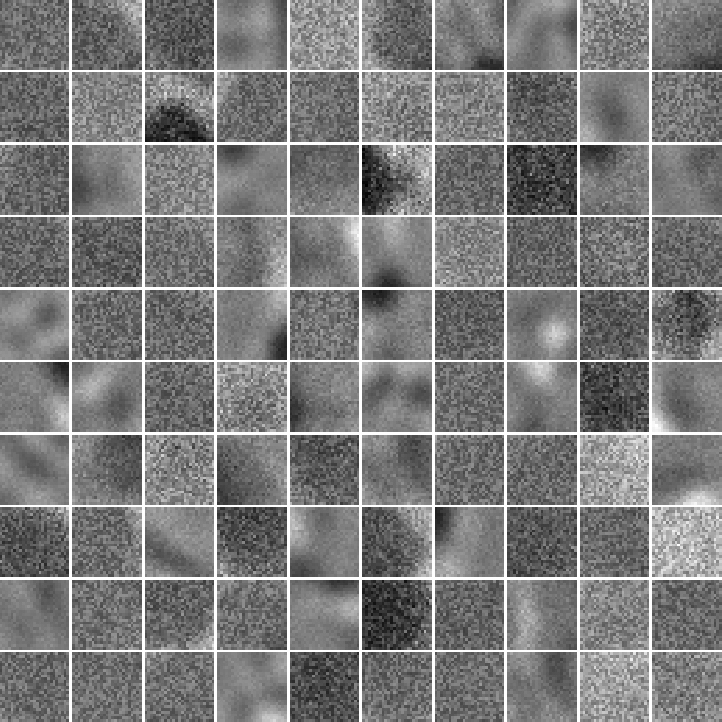

In this process, the hidden layer output of each layer network is the “depth feature” of the image. In order to make the deep neural network have the classification function, we need to use supervised learning to fine-tune the whole network to make the features correspond to the category. The specific method is to use the parameters of each layer before to build a complete deep neural network, and add an output layer at the end of the whole network to build a feedforward deep neural network, and then compare the output results with the data true value. The network parameters are adjusted according to their differences, so that the input samples can output their corresponding categories after a series of network mapping, that is, they have the ability to classify and identify samples.

Figure 7 shows a complete training process of stacker. On the left is the process of pre-training with unlabeled samples to construct the initial deep neural network; on the right is the process of fine-tuning the initial depth neural network with labeled samples to make it have the classification function.

Figure 7.

Depth neural network based on stack noise reduction automatic encoder. a. Pre-training; b. Fine-tuning.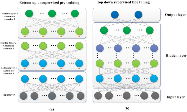

The fine-tuning depth neural network can be used to classify the samples. In the input layer, the sample data to be classified is input (there is no need to pollute the initial data in the classification task). After a number of preset intermediate layers, the sample features are automatically analyzed, and finally the classification results are output through the output layer. The target of the classification task in this paper is a result of dichotomy to detect whether the pixels corresponding to the input image block samples belong to brain tumor tissue.

2.4 Optimization of segmentation results

After the classification results of image blocks are obtained, the corresponding center pixels can be mapped to the corresponding categories according to the category label of each image block, so as to obtain the initial segmentation results. However, due to the use of the regional gray level of the image block as the classification basis, there may be false segmentation. As shown in Fig. 8, some normal brain tissues are also divided into the brain tumor regions with green marks.

Figure 8.

Initial segmentation results.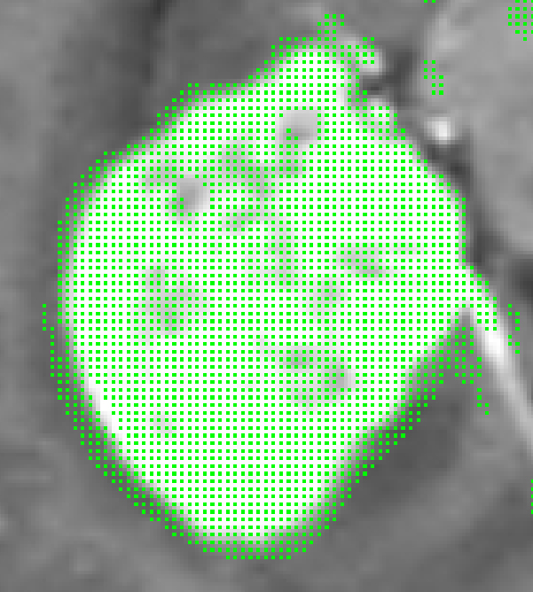

In order to eliminate the phenomenon of false segmentation, the initial segmentation results can be preliminarily processed by threshold segmentation. The threshold value is set according to the gray distribution of all the pixels classified as brain tumor tissue, and then the pixels that obviously do not belong to tumor tissue are deleted.

Figure 9 shows the results of threshold segmentation, Fig. 9a is the original image to be segmented; Fig. 9b is the binary image generated by the original image space by using the stacking automatic encoder, and the classification result is mapped to the original image space, that is, the initial segmentation result; Fig. 9c is the result of optimization processing by using the threshold segmentation method.

Figure 9.

The segmentation results were optimized. a. Original image; b. Initial segmentation result; c. Optimized result of threshold segmentation method.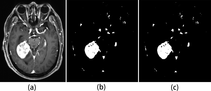

Figure 10.

Morphological optimization results. a. The results of threshold segmentation optimization; b. Morphological processing optimization results.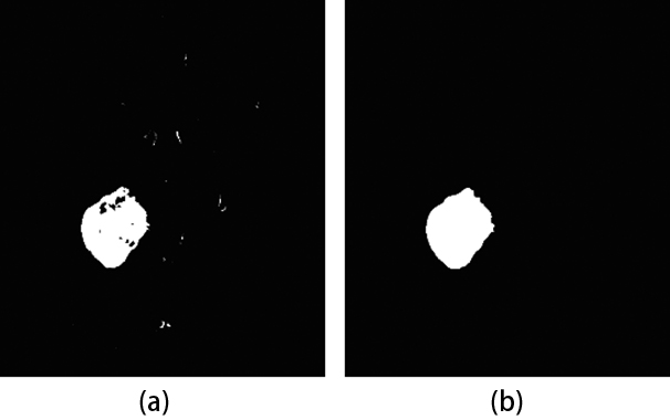

As can be seen in Fig. 9c, after optimization of the threshold segmentation method, the larger isolated patches in the initial segmentation results are basically eliminated. However, there are still some spots isolated outside the tumor area and interspace in the tumor area. According to the integrity and continuity of tumor tissue, it can be judged that these spots and spaces are obviously misclassification, which needs further optimization.

In order to get better segmentation results, we use the open and close operations of morphological processing methods to optimize the segmentation results. The main function of the open operation is to eliminate the bulge and isolated spots on the edge of the image, while the main function of the closed operation is to fill the gap and concave edge in the image. In this paper, in order to optimize the segmentation results of tumor tissue, the above two morphological operation methods will be combined. The results of morphological segmentation optimization are shown in Fig. 10.

3. Results and discussions

3.1 Parameter setting and experimental data

The experimental data in this study were provided by our hospital, including brain MRI cross-sectional images from 10 patients with brain tumors. All images have been processed by data format conversion, brightness enhancement and noise reduction [14]. Neurosurgery and imaging doctors manually depict the true value region of brain tumor as the reference standard for training sample labels and comparative experiments.

In the semantic based image segmentation, it is necessary to classify and identify the pixels of the image. Considering the integrity of brain tumor tissue, the gray value of corresponding region pixels should be continuous. Therefore, in the detection process, we take the pixel as the center, extract the gray value of all the pixels in the adjacent 25 $\times$ 25 area, and connect them into 625 dimensional gray vector in the order from top to bottom, as the input data of neural network. The feature vector extraction process of image block is shown in Fig. 11, in which the label is selected according to the real brain tumor region information determined by the doctor, and the coordinates are the position of the central pixel a in the original image, which is used to reconstruct the tumor region image after classification.

Figure 11.

Schematic diagram of the image block extraction principle.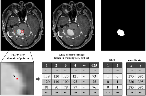

In the process of image block sampling, in order to save calculation cost and keep sample balance, different sampling rules are applied to the normal brain tissue and brain tumor area in the training samples. The normal brain tissue area is sampled every four pixels, and the brain tumor area is sampled once every other pixel. The category label and coordinates of the sampling points are recorded for each sampling.

In addition, considering that the construction of deep neural network requires a large number of training samples, in order to expand the number of training samples, and also to test the results of different brain tumor images segmentation by the method in this chapter, the experiment will use the “leave one” method for ten fold cross validation. Among the ten MRI images of brain tumor, one image is selected for testing in each round, and the other nine images are used as training set. The number of training samples and test samples collected in each round of experiment are shown in Table 1.

Table 1

Number of samples per round

Round	Training sample	Test sample
1	143300	70070
2	150900	65473
3	145000	81048
4	147500	65552
5	148000	42336
6	143100	70848
7	147500	76032
8	150200	17952
9	147400	46434
10	151000	55471

Through the above sampling method, each image block can get a 625 dimensional vector. As shown in Fig. 12, each dimension data in all image blocks is sorted, and 625 input layer nodes of stack noise reduction automatic encoder are input successively to generate the first layer neural network.

Figure 12.

Schematic diagram of the input form of the input matrix.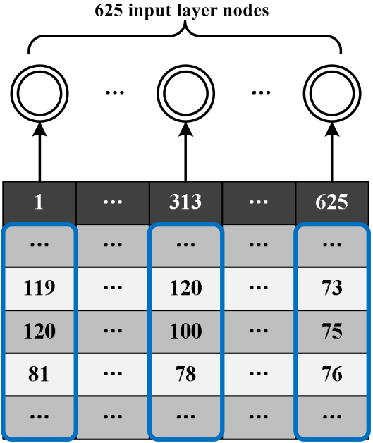

The random noise ratio of the initial input layer is set to 50% in order to enhance the robustness of the neural network after noise data reconstruction. In the process of further constructing the deep neural network, the following key parameters need to be set.

First of all, the number of intermediate layers and the number of nodes in each layer need to be determined. According to the empirical value, we give an assumed value of 100 for the number of nodes in each layer in advance, and then test the classification by setting different number of intermediate layers. Figure 13 shows the classification accuracy of each group of samples with different number of intermediate layers.

Figure 13.

Number of intermediate layers test.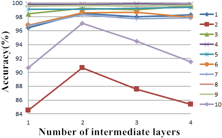

The lines with different colors in the figure represent different patient samples. Obviously, when the number of intermediate layers is set to 2, the recognition rate of most patient samples can reach a high level, especially for patient 2 and patient 10 with the lowest overall recognition rate. If we continue to increase the number of intermediate layers to 3 or 4 layers, the recognition rate of some patient samples can continue to improve, but the corresponding computational complexity will also increase. Therefore, in the subsequent experiments, the number of intermediate layers of deep neural network is set to 2 layers.

Second, three interrelated parameters need to be set: batch size, iteration and epoch (the Chinese translation names are batch size, iteration and period. Considering that the current Chinese translation is difficult to accurately express the meaning of parameters, the original English name is used for description later). Batchsize represents the number of samples in each training. Due to the problem that the number of samples is too large and the computer memory is insufficient in the training process of deep neural network, the running efficiency and utilization rate of memory can be effectively improved by limiting the number of samples participating in each training. Iteration is the number of iterations using batch size samples, while epoch represents a complete training using all samples in the training set. Therefore, the larger the value of batchsize set in training, the smaller the number of iterations (i.e. iteration value) required for a single epoch, and the total processing time and stability rate can be improved accordingly. However, with the increase of batchsize, the memory capacity required for a single iteration will also increase. Accordingly, more epochs are needed to obtain the best results. Therefore, the value of batchsize is very important. It needs to be tested according to the actual sample data and experimental environment, and then select a middle value that can balance the memory efficiency and memory capacity. Set the number of intermediate layers to 2 and the number of nodes to 100. Figure 14 shows the test results of training time under different values of batch size.

Figure 14.

Different batch training times for size value.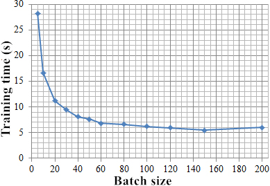

It can be seen that with the increase of the value of batchsize, the required training time decreases correspondingly. However, if the batchsize is too large, the memory overflow may not be calculated. Moreover, as the number of iterations required for a single epoch is reduced, more epochs are needed to obtain the same precision, but the overall running time is increased. Therefore, we choose a moderate batchsize value of 100 to limit the number of samples in a single training.

The value of iteration can be obtained automatically according to the total number of samples and the value of batch size. Next, we need to determine the number of epoch. When the value of batchsize is 100, Fig. 15 shows the influence trend of different epoch times on accuracy.

Figure 15.

Influence of different epoch values on accuracy.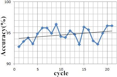

Generally speaking, the more epoch times, the higher the accuracy. However, with the increase of epoch times, the calculation time will also increase by multiple, and it is easy to over fit. Therefore, the range of values is generally limited to 10 $\sim$ 40 times. According to the results of our experiment, we set the number of epochs to 20 and 20 times respectively [15].

In addition, according to the suggestions in the literature, we add dropout parameter (loss rate) in the training process of deep neural network. Its function is to make a certain proportion of neural nodes stop working at each training time, so as to reduce the complexity of neural network, and prevent over fitting phenomenon. The parameter of dropout suggested in the literature is 0.5, that is, 50% of the neuron nodes are randomly closed in each training. But after the actual test, we found that the dropout parameter set to 0.4 can achieve better classification accuracy. Figure 16 shows the classification accuracy with different dropout parameter values [16].

Figure 16.

Dropout parameter test.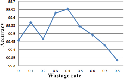

To sum up, in this experiment, we set the number of intermediate layers of deep neural network as 2 layers, the number of nodes in each intermediate layer is 100, and the number of single training samples is 100. In the pre-training process, the total number of training rounds for all samples is 15, and the number of fine-tuning is 20. In addition, the initial input layer noise ratio of stack noise reduction automatic encoder is 50%, and 40% nodes are randomly selected to stop responding in each training. Through pre-training and fine-tuning, the depth neural network based on stack noise reduction automatic encoder is obtained, and then the image block samples are classified.

3.2 Segmentation results of brain tumor tissue

In the previous chapter, stack noise reduction automatic encoder to build a depth neural network is used to classify all the image blocks in the MRI image to be segmented. Then, according to the category label of each image block, the central pixel points are mapped to the coordinate space of the original image one by one, and the binary image is reconstructed as the initial segmentation result.

Then, in order to get more accurate segmentation results, the initial segmentation results need to be further optimized. As mentioned above, the accurate segmentation of brain tumor tissue can be divided into three steps. Firstly, the depth neural network is used to detect the pixels belonging to brain tumor tissue, and the initial segmentation results of brain tumor are reconstructed in the original coordinate space. Then, the initial segmentation results are processed by threshold segmentation to remove the abnormal areas with large gray difference. Finally, the morphological processing method is used to optimize, eliminate the discontinuous small noise, fill the small space in the tumor area, and get the accurate segmentation results of brain MRI image. Figure 17 shows the results of each stage.

Figure 17.

The segmentation results of the three stages. a. Initial segmentation results; b. Threshold segmentation optimization results; c. Morphological processing optimization results.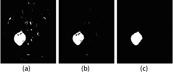

In order to more intuitively compare the changes of segmentation results in each step of processing, we list the segmentation accuracy of each patient sample in three stages, as shown in Table 2.

Table 2

Segmentation accuracy of different stages

Sample number	Initial segmentation	Threshold segmentation	Morphological optimization
1	98.49	99.65	99.88
2	90.64	99.31	99.95
3	99.24	99.60	99.93
4	99.82	99.72	99.75
5	99.09	99.21	99.56
6	98.58	99.52	99.83
7	98.26	99.68	99.95
8	99.65	99.82	99.88
9	99.62	99.71	99.75
10	97.05	99.45	99.96
Average value	98.044	99.567	99.844

Table 3

The result of segmentation compared with the true value

Aggregate	1	2	3	4	5	6	7	8	9	10
DL	9185	2280	5616	8595	9367	4068	4068	8815	8979	3653
GT	9312	2175	5712	9204	9450	5756	3946	8919	8815	3699

Figure 18 shows the comparison between the true value segmentation results of brain tumor regions of three patients and the segmentation results of this chapter. Among them, the real brain tumor area is manually described by neurosurgeons, as shown in Fig. 18b; the real brain tumor area manually labeled by doctors is mapped into a binary image as the true value segmentation result, as shown in Fig. 18c; the automatic segmentation results after secondary optimization in this method are compared, as shown in Fig. 18d. It can be seen that the brain tumor image segmented by the method proposed in this chapter is very close to the real result drawn by doctors.

Figure 18.

Comparison of the segmentation results. a. The image to be segmented; b. Manually labeled tumor area; c. True value segmentation result; d. Automatic segmentation result.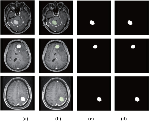

In order to more accurately calculate the approach degree between the method in this chapter and the true value, the segmentation results will be further evaluated by numerical evaluation index. Let the set of all pixels in the real brain tumor region be GT, and the set of all pixels in the brain tumor region segmented by this method is dl. The detection results are shown in Table 3.

The values in the table represent the number of pixels in the set. It can be seen that the number of DL and GT of all patients are very close. However, it should be noted that in the segmentation result DL, both the correct segmentation results belonging to the true value GT region and the wrong segmentation results not belonging to the GT region may exist. In the true value GT region, there are not only the regions correctly segmented by the method DL in this chapter, but also the regions not segmented. According to the interaction between the true value GT and the segmentation result DL, three evaluation indexes can be obtained.

Among them, true positive (TP) represents the correct pixel set of segmented tumor region, which is used to measure the correct number of segmentation results.

$\displaystyle TP=\{x(i,j)/x\in GT,x\in DL\}=GT\cap DL$ (9)

False positive (FP) represents the pixel set of non tumor areas determined as tumor tissue, which is used to measure the number of false positives in segmentation results.

$\displaystyle FP=\{x(i,j)/x\notin GT,x\in DL\}=\overline{GT}\cap DL$ (10)

False negative (FN) represents the set of pixels whose tumor area is determined as non tumor tissue, which is used to measure the number of missed judgments in segmentation results.

$\displaystyle FN=\{x(i,j)/x\in GT,x\notin DL\}=GT\cap\overline{DL}$ (11)

The performance of the segmentation algorithm can be measured more intuitively, and the proportion of the correctly detected tumor area in the actual tumor area can be measured by calculating the sensitivity, which is also called true positive rate or detection rate.

$\displaystyle\textit{SEN}=\frac{TP}{GT}$ (12)

Table 4 shows the calculation results of each evaluation index. Among them, the higher the true positive value, the better, and the less false positive and false negative value, the better. It can be seen that the segmentation results obtained by the method in this chapter are very close to the true value, and the average detection rate is 96.24%.

Table 4

The result of segmentation compared with the true value

Patient number	True negative	False positive	False negative	Sensitivity
1	9057	128	225	97.26
2	2155	125	20	99.08
3	5544	72	168	97.06
4	8539	56	665	92.77
5	8405	191	641	92.91
6	8318	49	483	94.51
7	3918	28	150	96.31
8	5666	163	90	98.44
9	8636	179	343	96.18
10	3621	32	78	97.89

The experimental results show that the proposed method has high sensitivity and good stability in the automatic segmentation of brain tumor tissue.

4. Conclusions

In this paper, we use deep learning method to solve the problem of semantic based medical image segmentation. A deep neural network is constructed by stacking automatic noise reduction encoder (SDA) to learn and classify image pixel blocks, and then realize automatic segmentation of regions of interest. Firstly, the unlabeled image block samples are used to train the stacked noise reduction automatic encoder, and the deep features of the image are learned and extracted to construct the initial depth neural network model; then, the labeled samples are used to fine-tune the initial depth neural network model, and the deep layer features of the image are corresponding to the category to obtain the depth neural network model with classification function; then, the depth neural network model with classification function is obtained. Finally, threshold segmentation and morphological methods are used to optimize the initial results to obtain accurate segmentation results. The experimental results show that the average segmentation accuracy is improved to 98.04% (before optimization) and 99.84% (after optimization), and the sensitivity is increased to 96.24%. At the same time, the running speed is also greatly improved compared with the traditional machine learning method.

Footnotes

Conflict of interest

None to report.

References

Parekh

Jacobs

. SU-F-R-05: multidimensional imaging radiomics-geodesics: a novel manifold learning based automatic feature extraction method for diagnostic prediction in multiparametric imaging. Medical Physics, 2016, 43(6): 3373–3374.

Wang

Wen

, et al. A deep learning based feature extraction method on hyperspectral images for nondestructive prediction of TVB-N content in pacific white shrimp (litopenaeus vannamei). Biosystems Engineering, 2019, 178: 244–255.

Sourati

Gholipour

, et al. Intelligent Labeling Based on Fisher Information for Medical Image Segmentation Using Deep Learning. IEEE Transactions on Medical Imaging, 2019: 2642–2653.

Liu

Taniguchi

Tanaka

, et al. Visualization of driving behavior based on hidden feature extraction by using deep learning. IEEE Transactions on Intelligent Transportation Systems, 2017, PP(9): 1–13.

Antropova

Huynh

Giger

. A deep feature fusion methodology for breast cancer diagnosis demonstrated on three imaging modality datasets. Medical Physics, 2017, 44(10).

Zhang

Ding

. Deep learning-based remaining useful life estimation of bearings using multi-scale feature extraction. Reliability Engineering and System Safety, 2019, 182(FEB.): 208–218.

Daoxi, Huosheng, Pan, et al. Pose estimation-dependent identification method for field moth images using deep learning architecture. Biosystems Engineering, 2015.

Sun

Bourennane

. Hyperspectral image classification with unsupervised feature extraction. Remote Sensing Letters.

Wang

Guo

Luo

. A new automated spectral feature extraction method and its application in spectral classification and defective spectra recovery. Monthly Notices of the Royal Astronomical Society, (4): 4311–4324.

10.

Arora

Rai

Raman

. Deep feature-based automatic classification of mammograms. Medical and Biological Engineering and Computing, 2020, 58(6): 1199–1211.

11.

Cui

Zhang

Liu

, et al. A deep learning algorithm for one-step contour aware nuclei segmentation of histopathological images. Medical and Biological Engineering and Computing, 2018, 67(dec): 1–8.

12.

Yen

Sun

. An android mutation malware detection based on deep learning using visualization of importance from codes. Microelectronics Reliability, 2019, 93(FEB.): 109–114.

13.

D’Isanto

Polsterer

. Photometric redshift estimation via deep learning – Generalized and pre-classification-less, image based, fully probabilistic redshifts. Astronomy and Astrophysics, 2018, 609.

14.

Jun, Wang, Jingwei, et al. Road network extraction: a neural-dynamic framework based on deep learning and a finite state machine: international journal of remote sensing: Vol 36, No 12. International Journal of Remote Sensing, 2015, 67(dec): 1–8.

15.

Cambria

Huang

Kasun

LLC

, et al. Extreme learning machines [trends and controversies]. IEEE Intelligent Systems, 2013, 28(6): 30–59.

16.

Lei

Zhu-Hong

Yu-An

, et al. An efficient approach based on multi-sources information to predict circRNA-disease associations using deep convolutional neural network. Bioinformatics, (11): 13.