A bottom-up search algorithm for size-constrained partitioning of modules to generate configurations in modular robots

Abstract

We consider the problem of partitioning a set of modules for efficient and dynamic shape or configuration generation in modular robotic systems, where the size of any configuration formed by the modules is constrained by a maximum, user-provided value denoted by $n_{max}$ . The objective is to determine the best partition of the module set that gives the highest utility to the modules. This problem is non-trivial as the set of partitions that needs to be explored grows exponentially with the number of modules and an exhaustive search in the space of partitions makes the problem intractable. To address this problem, we propose a branch and bound based search algorithm, called bottomUpCSGSearch, which is able to intelligently prune the unpromising search space and find the best partition of the modules in a reasonable amount of time. We have provided analytical results related to the completeness, anytime nature and time complexity of our proposed algorithm. Our experimental results show that our proposed algorithm performs better in terms of number of nodes explored (up to $2^{8}$ times fewer nodes explored) and the time required to find the best partition (improvement up to the order of $10^{4} ms$ ) than existing comparable algorithms. We have simulated with different number of modules and different values of maximum coalition size of a modular self-reconfigurable robot (MSR) called ModRED, and, shown that our algorithm takes nominal time to find the best solution.

Keywords

Modular robots configuration generation coalition structure formation algorithm

1. Introduction

Modular self-reconfigurable robots (MSRs) are composed of individual modules, which can change the connections among themselves to form different shapes or configurations. The proposed algorithms in this paper are developed for homogeneous modular robotic systems [5,32], where all modules are identical in their construction; they can be used for heterogeneous modular robots [12,19] as well. The main advantage of using MSRs is that the modules can change the connections among themselves to form different shapes and transition from one shape to another depending on the current environment and current task at hand. In this paper we try to answer the following research question that we call the partitioning problem for configuration generation: how to identify the best partitioning of modules for forming any configuration, while maximizing some predefined objective function. Finding the best partitioning of modules for forming shapes or configurations is a non-trivial problem, as the number of possible partitions is exponential with the number of modules involved. Moreover, the computation becomes further complicated if we include uncertainty in the mobility and connections of modules, which are practical considerations for any physical modular robot operating in an unknown environment.

Fig. 1.

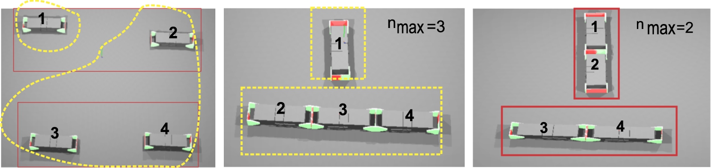
An example illustrating the configuration generation process: (left) shows the initial arrangements of the modules, (middle) shows the best partitions calculated, (right) shows the final configurations of the modules.

To address these challenges, in this paper we have proposed a search algorithm while using concepts from cooperative game theory [21], called coalitions and coalition structures. A coalition is a group of autonomous agents (modules in our scenario) which work together towards achieving a common goal. From the MSR perspective, a coalition is a configuration formed by a set of modules which are connected and can maneuver as a single entity. A coalition structure corresponds to disjoint and exhaustive sets of coalitions (connected modules) which represent all shapes or configurations formed by a set of MSRs. In this paper, we have modeled the best configuration generation problem as the best coalition structure generation problem; as finding the best coalition structure will give us the best partition of modules, i.e., the best set of possible configurations. Coalition structure generation and searching for the best coalition structure are well-known NP-complete problems [26] and exhaustively searching for the set of all possible coalition structures becomes computationally prohibitive even for a relatively small number of coalitions. Coalition structure generation problems have been proposed for real-world scenarios like voting, or for task completion while maximizing resource allocation criteria [29]. However the direct implementation of the previously developed algorithms for the best coalition structure generation for virtual agents, such as in [22,23], is infeasible, due to mechanical constraints, communication constraints, and uncertainty in robots’ movements as well as in the environment.

Each configuration or shape needs a specific number of modules in it, denoted by $n_{max}$ , to form the configuration [15]. In [15], the authors have mentioned that for reconfiguration from one shape to another, both shapes require exactly the same $(n_{max})$ number of modules present, connected together. If $n_{max}$ modules are together forming a shape, then the probability of forming the desired shape is higher. On the other hand, if there are more or fewer modules than $n_{max}$ present to form the desired shape, then the formation is not completely successful – either the shape will not be complete (if there are <n_max modules) or it will be bigger in size and also different in shape from the desired configuration (if there are >n_max number of modules present). Therefore having more or fewer modules will lead to undesired configuration formation. To incorporate this criterion into our approach, we have proposed a variant of the classical coalition structure generation problem called size-constrained coalition structure generation. In this approach, each coalition’s worth or value is determined by the number of modules it has – if there are exactly $n_{max}$ modules then the coalition will receive the highest value; otherwise its value will be diminished. Many real-world domains, such as sports teams or judging committees, are constrained by a similar maximum size determined by the game or the competition rules. As a motivating example, we consider a scenario where a set of singleton ModRED modules [3] are dropped from a vehicle in an extra-terrestrial environment. The task for them is to form shapes (or configurations) to inspect parts of the environment, such as volcanic craters. To access a specific region of the environment, not any configuration of any size can be formed due to size and shape restrictions. Let us assume that the maximum size any configuration can have is $n_{max}$ . Now the modules need to find the best partition among themselves which also restricts the maximum size of any configuration to $n_{max}$ .

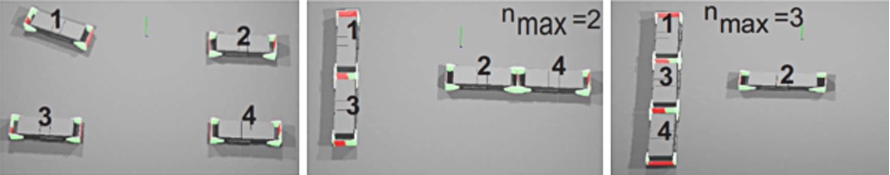
An example of the working procedure of our algorithm is shown in Fig. 1, where number of modules $| A | = 4$ and $n_{max}$ is varied between 2 and 3. Initially modules are randomly distributed as singletons (Fig. 1 (left)). By using our proposed algorithm, modules decide what coalitions they should form among themselves, as shown in Fig. 1 (left), with red and yellow lines. Figure 1 (middle) and (right) show these coalitions being realized as MSR configurations, while using any of the available MSR reconfiguration techniques [15]. Thus by appropriate partitioning of the modules, we can find the best configurations. Though we have implemented our algorithms for configuration generation in a chain-type modular robotic system, named ModRED [3,13], these algorithms can be used for other types of modular robots, e.g., lattice [16] and hybrid [18], as well. Our experimental results show that our proposed bottomUpCSGSearch algorithm explores up to $2^{8}$ times fewer nodes than the existing CSG-search algorithms. An improved run time, up to the order of $10^{4}$ ms faster than existing CSG-based partitioning algorithms, is also reported.1

Some of the results presented in this paper have been previously published in [9].

The rest of the paper is structured as follows: Section 2 provides an overview of existing literature on modular robot reconfiguration and coalition structure graph search. It also introduces the modular robot platform used as a target application for validating the results in this paper. Section 3 introduces the dynamic partitioning problem in MSRs. Next, in Section 4, we present the bottomUpCSGSearch algorithm. In Section 5, we describe the experimental results of our algorithm, and finally we present conclusions.

2. Related work

We discuss previous similar studies in this section. The literature is divided into the following subsections.

Reconfiguration: Over the past decade, many approaches were proposed for modular robot reconfiguration. An overview of different control strategies can be found in [30]. Self-reconfiguration in modular robots is a NP-hard problem [15]. This problem has been solved using search-based [4,33], control-based [4,7] and task-based techniques [17]. Our work in this paper can be used in conjunction with any of these reconfiguration techniques as it enables the modules across different disjoint configurations to identify the best set of modules to form the goal configurations with the highest suitability, for performing the MSR’s current task, such as navigation [11].

Coalition Structure Search: Cooperative or coalition game theory gives a set of techniques that can be used by a group of agents to form teams or coalitions with each other [21,26]. A coalition structure graph (CSG) is usually used to represent the set of all possible coalition structures among a set of agents in a systematic and hierarchical manner. Searching for the best coalition structure within a CSG is a NP-complete problem [26].

Heuristic [25] and anytime [34] algorithms were proposed to solve the problem of finding the best coalition structure. Though heuristic algorithms scale up well with higher numbers of agents, the algorithms take a significant amount of time to find a good solution. Anytime algorithms alleviate this problem, but they can end up searching the whole search space, which is infeasible, due to large time complexity $(O (n^{n}))$ . Sandholm [26] has proved that all possible coalitions can be found in the first two levels of the CSG and proposed an anytime algorithm exploiting this property of the CSG. Rahwan [22] proposed an anytime, dynamic programming based approach called IDP which reduced the space complexity from a previous dynamic programming based approach [24]. Genetic algorithms have been used to implement these types of heuristic solutions [27]. Shehory and Kraus [28] have proposed a decentralized greedy algorithm which takes into account only those coalitions which have size less than a permitted value. In addition to the techniques in these solutions, our approach considers uncertainty while forming coalition structures, as it is an essential aspect of modular robot configuration generation.

Configuration Generation: In one of our earlier works [8], we proposed an anytime algorithm for configuration generation which takes the maximum value of permitted coalition size $(n_{max})$ as input and significantly reduces the time and space complexity compared to previously proposed configuration generation techniques, to find the optimal coalition structure, similar to [28]. In this work only those coalitions are searched which have sizes less than or equal to $n_{max}$ . In another earlier study, we used a graph partitioning approach for configuration generation [6] without taking uncertainty into account. In our more recent work, we have used CSG to find the best coalition structure [10]. Our work in this paper is an improvement over our previous work described in [10].

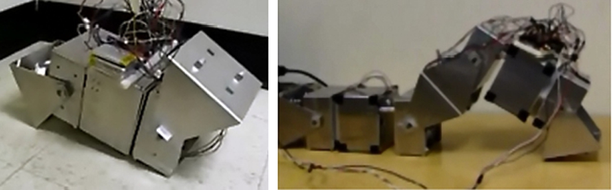
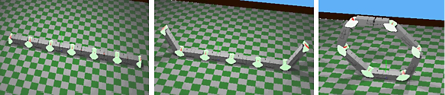
Currently we are building a MSR called ModRED [3,13]. ModRED has 4 degrees of freedom (3 rotational and 1 translational); this allows each module to rotate along its long axis as well as extend along that same axis. The combination of different DOFs enables ModRED to achieve a higher flexibility in motion, while maneuvering through tight spaces. Figure 2 shows the ModRED modules and their sensory details and two modules doing an inchworm-like motion. Each ModRED module uses two Arduino Fio (ATmega328P) micro-controllers for computational purposes. Power for the ModRED modules comes from a rechargeable lithium-polymer battery pack. Inertial Measurement Units (IMU) using Attitude Heading Reference System (AHRS) are used to determine the orientation of the modules. ModRED modules communicate among each other using XBee modules. For proximity sensing, each module is equipped with an infrared (IR) sensor. The movement of ModRED modules in fixed configurations is achieved through pre-defined gait tables [2]. Figure 3 shows simulated ModRED modules in the Webots simulator in chain and ring configurations.

Fig. 2.

ModRED hardware: (left) A single module and (right) Two modules doing inchworm-like motion.

Fig. 3.

Simulated model of 6 ModRED modules re-configuring from snake to ring shape.

Fig. 4.

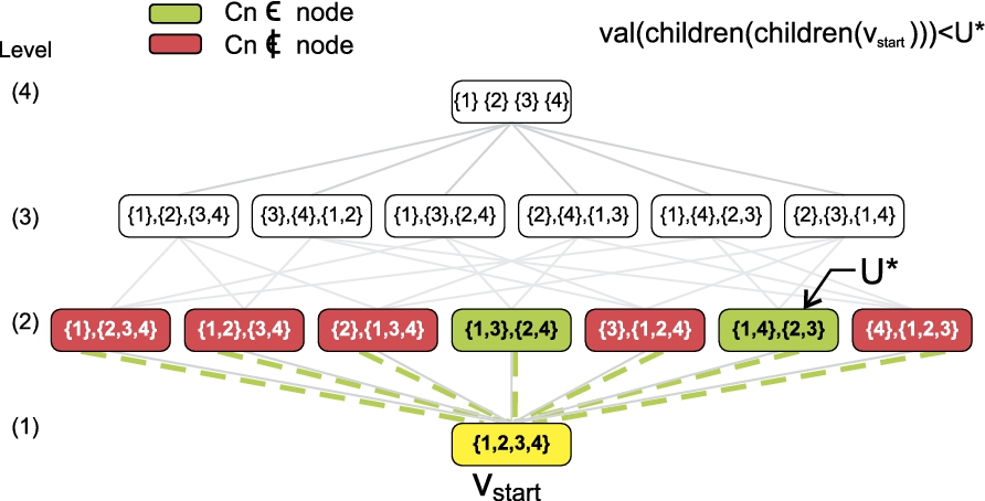
Coalition structure graph (CSG) with 4 agents.

3. Dynamic partitioning of modules: Preliminaries

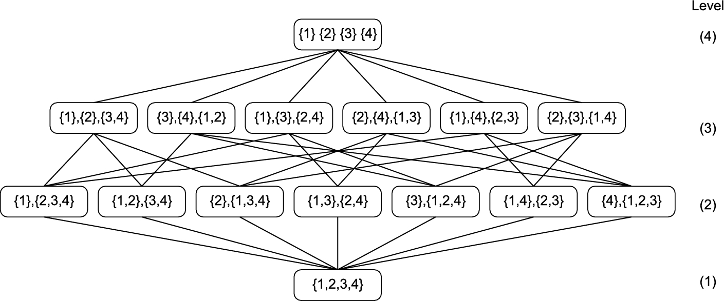
Let A be a set of modules. $A_{i} = {a_{i_{1}}, a_{i_{2}}, a_{i_{3}}, \dots, a_{i_{| A_{i} |}}}$ where ${a_{i_{j}}, a_{i_{j + 1}}}$ , $j = {1, \dots, | A_{i} | - 1}$ is the set of physically coupled modules in $A_{i}$ . When $| A_{i} | = 1$ , the MSR is a single module – we call it a singleton. Let $Π (A)$ be the set of all partitions of A. By a partition of a set A we will mean a collection of nonempty, pairwise disjoint sets whose union is A. The sets into which A is partitioned are called the classes of the partition [31]. The number of partitions of set A is exponential in $| A |$ , and this number is denoted by bell numbers $B_{| A |}$ [31], where $B_{| A |} = | Π (A) |$ . Also, let $CS (A) = {A_{1}, A_{2}, \dots, A_{k}} \in Π (A)$ denote a specific partition of A, which is called a coalition structure; note that $A_{i} \subseteq A$ is the i-th MSR in that coalition structure. A systematic way to go about analyzing the partitions in $Π (A)$ is provided by a hierarchical graph structure called a coalition structure graph (CSG) [21]. A CSG with 4 agents is shown in Fig. 4. CSG nodes are organized into levels. Level l indicates that every node in level l in the CSG has exactly l subsets or coalitions as its members. CSGs offer a structured way of exploring coalition structures because a node at level $l + 1$ can be generated by breaking up a coalition from a node at level l.2

²
In this paper, we assume that initially all the modules are singletons.

In a CSG, each partition $CS (A) \in Π (A)$ is called a coalition structure and appears as a node in the CSG. The parts or subsets of a partition are called coalitions, denoted by $A_{i}$ . Each coalition $A_{i}$ has a value associated with it that can be referred to as a virtual reward received by the agents in that coalition for coming together to perform the task at hand. The value function is denoted by $Val : A_{i} \to ℜ^{+}$ . The value function assigns to each coalition $A_{i}$ a real positive number corresponding to a virtual reward that the coalition can obtain for performing its assigned task. Our value function is modeled in a way such that it is beneficial for agents to form coalitions up to a certain coalition size $n_{max}$ but this benefit starts diminishing for coalition sizes that are larger than $n_{max}$ .

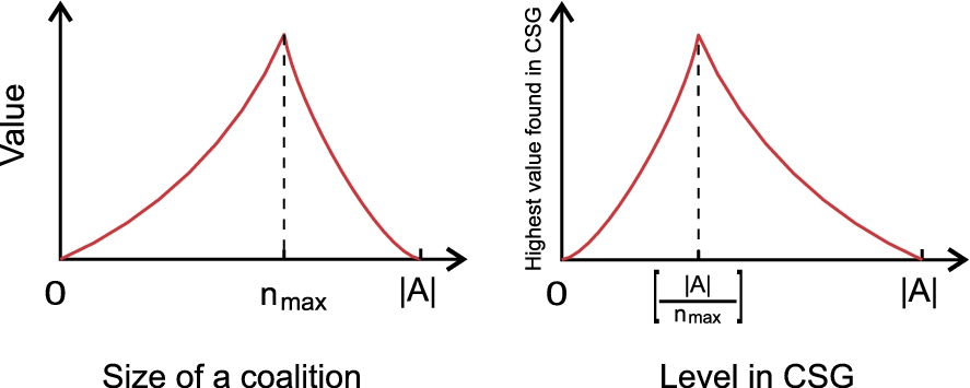
Size-Constrained Value Function: Each configuration needs exactly $n_{max}$ number of modules to form that particular configuration. But if $n_{max}$ number of modules are not present there, then forming that particular shape is impossible. To incorporate this, we have developed a size-constrained value function, which is illustrated in Fig. 5 (left) and represented by: $\begin{matrix} (1) & Val (A_{i}) = \{\begin{matrix} | A_{i} |^{k}, & if | A_{i} | ⩽ n_{max} \\ e^{- (| A_{i} | - n_{max})} \times n_{max}, & otherwise \end{matrix} \end{matrix}$ where k is any integer >1. The above value function is super-linear, i.e., $Val (| A_{i} | + 1) - Val (| A_{i} |) > Val (| A_{i} |) - Val (| A_{i} | - 1)$ ; which ensures that larger coalitions are better and obtain higher rewards, up to a size of $n_{max}$ , as it is taking the tally towards the number of modules required to form that configuration. $n_{max}$ denotes the maximum allowable size of a coalition; it is given as input to our algorithm and it does not change the operation of the algorithm. Our value function gives preference to larger coalitions only up to a certain size $n_{max}$ , beyond which larger coalitions are penalized by yielding lower values. The preferred size of a coalition is relevant to the task assigned to the MSR. The value of a coalition structure, $CS (A)$ , is given by the summation of the values of coalitions comprising it, i.e., $Val (CS (A)) = \sum_{A_{i} \in CS (A)} Val (A_{i})$ . Evidently, if forming coalitions incurred no cost, the most suitable partition for a set of agents is the one that maximizes $Val (CS (A))$ . For example, $Val ({1, 2}, {3, 4}) = Val ({1, 2}) + Val ({3, 4})$ . The size of coalitions ${1, 2}$ and ${3, 4}$ is 2. In Eq. (1), if we assume $k = 2$ and $n_{max} = 2$ , then $Val ({1, 2}, {3, 4}) = 2^{2} + 2^{2} = 8$ .

Fig. 5.

left: An illustration of the size-constrained value function; right: An illustration of the effect of this value function on finding higher utility nodes in the CSG.

An illustrative example scenario, where the size-constrained value function can be used, is shown in a snapshot of ModRED from the Webots simulator in Fig. 3 (right). If the desired motion of the MSR is to cross an obstacle while in a ring shape, which needs 6 modules to give the MSR sufficient traction for its rolling motion, then the value of $n_{max}$ is set to 6. As the focus of this paper is on determining the best coalition structure, the problem of determining the optimal $n_{max}$ is not considered further in this paper.

Uncertainty in Configuration Formation. Unexpected motion and alignment of the robot modules can cause ModRED’s behavior to deviate from ideal operation. Following [10], we have considered three major sources of uncertainty under this category that could affect the mobility of the modules and consequently the configuration generation process. The uncertainty model is summarized below:

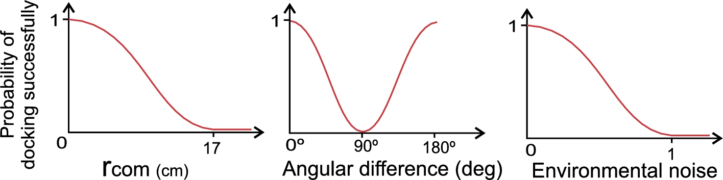
(i) Distance uncertainty is the uncertainty arising out of the distance required to be traversed by a pair of MSRs before docking with each other. As the modules do not know the features of the terrain (such as obstacles between them) beforehand, successful alignment and docking of the modules’ end connectors becomes more uncertain with higher distance between them. The distance uncertainty is modeled as a half-Gaussian distribution $N (μ_{du}, σ_{du})$ as shown in Fig. 6 (left).

(ii) Alignment uncertainty is the uncertainty arising out of the angle each MSR in a pair of docking MSRs needs to rotate before they can align with each other. As ModRED modules have docking faces at two ends [14], if the rotational difference between them is close to 0° or 180°, then it is easier for them to align and dock; they are most unaligned when the rotational difference between them is close to 90°. Alignment uncertainty between two modules is modeled as a Gaussian distribution, $N (μ_{au}, σ_{au})$ , as shown in Fig. 6 (middle).

(iii) Environment uncertainty is the uncertainty arising from the operational conditions in the environment due to factors such as terrain conditions, surface friction, etc. that affect the movement of a pair of MSRs while moving towards and docking with each other. The uncertainty is modeled as a multi-variate half-Gaussian distribution $N (μ_{eu}, σ_{eu})$ , as shown in Fig. 6 (right).

Fig. 6.

Probability of a pair of MSRs to dock successfully with each other for (left) distance between the MSRs, (middle) angular difference between the MSRs, and, (right) environment noise values [10].

To combine the Gaussians representing the motion uncertainties, a weighted mean with variance is considered [20], where weights are inverse of the variance estimates.3

According to the central limit theorem, any sum and/or average of samples from any random distribution with finite mean and standard deviation will always be approximately Gaussian.

These weights are denoted by

w_{du}

w_{au}

, and

w_{eu}

respectively. The weighted mean of the three Gaussians then gives the total motion uncertainty, expressed as a probability, for forming any coalition

A_{i}

by connecting its member modules, as given below:

\begin{matrix} (2) & prob (A_{i}) = \frac{(w_{du} \cdot p_{du} + w_{au} \cdot p_{au} + w_{eu} \cdot p_{eu})}{w_{du} + w_{au} + w_{eu}}, \end{matrix}

where

p_{du} \in N (μ_{du}, σ_{du})

p_{au} \in N (μ_{au}, σ_{au})

and

p_{eu} \in N (μ_{eu}, σ_{eu})

, and,

w_{du} = \frac{1}{σ_{du}^{2}}

w_{au} = \frac{1}{σ_{au}^{2}}

w_{eu} = \frac{1}{σ_{eu}^{2}}

Expected Cost functions. When a set of modules need to form a configuration, they move towards each other, the end modules align with the other’s docking faces and perform the connection operation [14] to finally form the configuration. To perform these operations, modules have to spend a considerable amount of battery power. Therefore the modules which are going to form a new configuration should be chosen in such a way that they expend less energy in moving and aligning. We have represented the energy expended by modules as the cost to generate configurations. While searching for the best coalition structure, modules not only need to find the coalition structure which has highest value, but also which incurs minimum cost.

Let $cost (A_{i})$ denote the cost of forming a coalition $A_{i}$ . $cost (A_{i})$ is defined as the cost of connecting singleton modules in a chain configuration. We denote the expected cost of forming coalition $A_{i}$ as: $\overline{cost} (A_{i}) = cost (A_{i}) \times (1 - prob (A_{i}))$ . This indicates that if the probability of modules connecting together in a coalition is higher, then the corresponding cost will be lower and vice-versa. Going further, we denote the expected cost of coalition structure $CS (A)$ as: $\overline{cost} (CS (A)) = \sum_{A_{i} \in CS (A)} \overline{cost} (A_{i})$ .

For notational convenience, we denote expected utility of a coalition structure $CS (A)$ as $\overline{U} (CS)$ where $\overline{U} (CS) = Val (CS (A)) - \overline{cost} (CS (A))$ ). Then, the optimal coalition structure is given by ${CS}^{*} = {argmax}_{CS \in Π (a)} \overline{U} (CS)$ . Based on the above formulation, we can now formally define the partitioning problem for modular robots as follows:

Definition 1.

Coalition Size-Constrained Partitioning Problem: Given a set of modules A and an initial coalition structure ${CS}_{old} (A) = {A_{1}^{old}, A_{2}^{old}, \dots, A_{k}^{old}}$ in which they are deployed (e.g., all singletons), find a new partition (or coalition structure) $CS (A) = {A_{1}^{new}, A_{2}^{new}, \dots, A_{k^{'}}^{new}}$ such that the following objective is maximized: $\max_{CS (A) \in Π (A)} \overline{U} (CS)$

An example of the configuration generation using the objective function, is shown in Fig. 1. Figure 1 (left) shows an initial configuration of ModRED, where the modules are randomly distributed as singletons. $n_{max}$ is given as input, varied between 2 and 3. Following the proposed bottomUpCSGSearch algorithm, modules determine the best configuration, which happens to be ${{1}, {2, 3, 4}}$ when $n_{max} = 3$ and ${{1, 2}, {3, 4}}$ when $n_{max} = 2$ . Modules then move and align themselves to form the new coalitions and finally the planned configurations are formed (Fig. 1 (middle), (right)).

In the rest of the paper, for the sake of legibility, we slightly abuse notations by referring to expected utility and expected cost as utility and cost respectively. Finally, we use two notations for convenience in our CSG search algorithm – a coalition of size $n_{max}$ is denoted by $C_{n}$ and the level in the CSG that contains the maximum number of coalitions of size $n_{max}$ is denoted by $l_{n_{max}}$ , where $l_{n_{max}}$ = $⌊ \frac{| A |}{n_{max}} ⌋$ .

4. Search algorithm: bottomUpCSGSearch

Size-based Partitioning of CSG. Our value function assigns the highest value to the coalitions which have size $n_{max}$ . From coalition size 0 to $n_{max}$ , the value of a coalition increases in a super-linear fashion, as discussed earlier, whereas beyond size $n_{max}$ , the value of a coalition decreases exponentially (Fig. 5 (left)). As the utility of a coalition structure depends on the values of its member coalitions, the coalition structure with member coalitions having sizes $n_{max}$ will most likely be part of the best coalition structure. Our algorithm is designed towards exploiting this property of the value function. The objective of our proposed CSG search algorithm is to target the search towards nodes (coalition structures) in the CSG that include coalitions of size $n_{max}$ ( $C_{n}$ ).

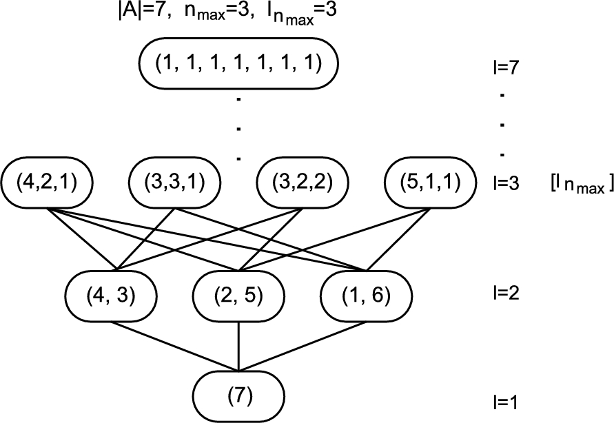
Sandholm [26] has proved that in level 2 of the CSG, we can get all the possible coalitions. This means after expanding the bottom most node of the CSG, we can encounter all the coalitions with size $n_{max}$ . And we have already discussed earlier that coalitions with size $n_{max}$ earn the highest value; therefore coalition structures containing these coalitions, will have higher chance to be the best coalition structures. This is the main insight of our approach. Therefore, a search starting from the bottom and going upwards in the CSG (bottom-up CSG search), unlike our previous approach [10], will be faster and more efficient. Possible sizes of the member coalitions in any coalition structure can be found by the integer partitions [1] of the total number of modules $| A |$ . For example, there are 5 possible integer partitions of number 4, which are $(4), (3, 1), (2, 2), (2, 1, 1), (1, 1, 1, 1)$ . From the coalition structure perspective, each integer partition indicates the sizes of the member coalitions in any coalition structure. For example, in Fig. 4, level 1 of the CSG consists of only 1 node (coalition structure), which is ${1, 2, 3, 4}$ . This coalition structure consists of only one coalition of size 4, which is the first integer partition of number 4–(4). In level 2, all the coalition structures have 2 coalitions in them. Either these coalitions have sizes 3 and 1 (such as ${{2}, {1, 3, 4}}$ ) or 2 and 2 (such as ${{1, 2}, {3, 4}}$ ). Thus the nodes in a CSG can be clustered according to their underlying integer partitions.

Fig. 7.

An abstraction of the CSG for $| A | = 7$ agents showing the partitions of A that are inspected at each level. Note that at level l, A has different partitions with exactly l parts or subsets. With $n_{max} = 3$ , the maximum number of $C_{n}$ -s (coalitions of size 3) are at level $l_{n_{max}} = 3$ .

Algorithm 1

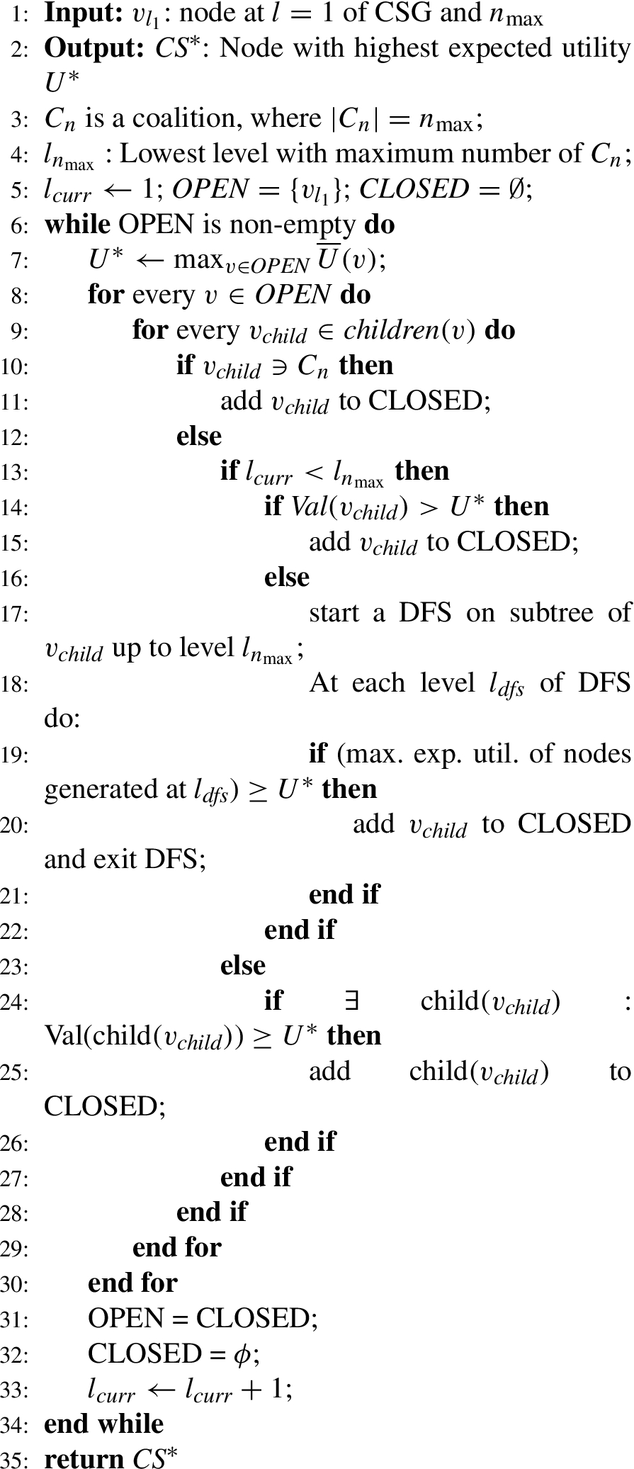
bottomUpCSGSearch Algorithm

An illustration of the partitioned CSG with $| A | = 7$ and $n_{max} = 3$ is shown in Fig. 7. This is a size based partitioning graph of the CSG. Each node represents the partition size of a coalition structure. For example, node (7) represents that the coalition structure corresponding to this partition has only one coalition in it with size 7; similarly the node $(3, 3, 1)$ represents all the coalition structures which have 3 coalitions in them with sizes 3, 3 and 1 respectively. As $n_{max}$ is 3, the highest valued coalition structures can be found under the $(3, 3, 1)$ partition. Coalition structures corresponding to that partition can be generated from coalition structures of two different partition sizes, viz., $(4, 3)$ and $(1, 6)$ . Note that all the coalition structures of size partition $(4, 3)$ have one coalition of size $n_{max}$ but that is not the case for $(1, 6)$ ; however, both of the partitions can generate coalition structures of highest possible value. Figure 5 (right) shows that because of our proposed value function, the highest valued coalition structures, i.e., the coalition structures which have a maximum number of $n_{max}$ -sized coalitions in them, can be found in level $⌊ \frac{| A |}{n_{max}} ⌋ (l_{n_{max}})$ in the CSG. Our proposed algorithm takes these factors into account and the search is designed accordingly.

Discussion of the bottomUpCSGSearch algorithm. In [22], the authors have shown that if it is impossible for some node in the CSG to lead to the best coalition structure, then those unpromising nodes can be pruned right away and the search process can be made faster. However, identifying these unpromising nodes is a challenge. We have employed two different pruning strategies to reduce the search space by eliminating the unpromising nodes as soon as we encounter them. The main search procedure is shown in Algorithm 1. As the name suggests, the search (called bottomUpCSGSearch) for the best coalition structure starts from the bottom-most node of the CSG. The bottom-most node (coalition structure) contains only one coalition in it – the grand coalition, i.e., every module is part of this coalition. All the nodes which need to be explored further are kept in a data structure called $OPEN$ . Initially the bottom-most node of the CSG is kept in $OPEN$ . At every level, all the children nodes of the nodes stored in the $OPEN$ data structure are generated.4

⁴

Children nodes of node v in level l of the CSG, denoted by $children (v)$ , are the nodes connected via edges to node v in the CSG in level $l + 1$ .

If a child node contains a

C_{n}

(a coalition having size

n_{max}

), it is immediately added to

CLOSED

for future expansion (lines 10–11). If a child node does not contain any

C_{n}

, it might still lead to the optimal coalition structure. To detect the suitability of a generated child node not including

C_{n}

, we check if the current level,

l_{curr}

, being explored in the CSG is less than

l_{n_{max}}

Let $U^{*}$ denote the highest utility found. As utility is the difference between the value and cost of a coalition structure, if the value of any coalition structure is less than $U^{*}$ , then the utility of that coalition structure will always be less than $U^{*}$ . This is the main insight behind developing our first pruning strategy, the fitness test. This pruning strategy is applied only if the current level $l_{curr} < l_{n_{max}}$ . For any newly generated coalition structure $CS$ in level $l_{curr} (< l_{n_{max}})$ , we first check whether the value of this coalition structure exceeds $U^{*}$ or not. If $Val (CS) ⩾ U^{*}$ , then it would make sense to explore the node $CS$ further; therefore $CS$ is added to the set $CLOSED$ for future expansion (lines 13–15). On the other hand, if $Val (CS) < U^{*}$ , i.e., the value of the coalition structure is already below the best utility found thus far, then it is evident that the utility of this node will be less than $U^{*}$ . Therefore exploring all of its children nodes for further expansion and inspection will not be beneficial. These are unpromising nodes. For this type of nodes, we only explore their descendants up to depth $l_{n_{max}}$ . While performing this depth-first search (DFS) of the unpromising node $CS$ , if any of the descendants has a value $> U^{*}$ , then we add $CS$ to $CLOSED$ for future expansion, as it can lead to a node that has utility better than the maximum utility obtained till then (lines 16–20). Otherwise, we just continue the search along the child (expanded node) that has the highest utility amongst all its generated siblings. If none of the descendants of $CS$ , till level $l_{n_{max}}$ , has higher value than the current highest utility, then $CS$ is automatically pruned.

Figure 5 (right) suggests that up to level $l_{n_{max}}$ the value of coalition structure increases, and beyond $l_{n_{max}}$ level, the value decreases. Therefore for expanding the nodes in any level $l_{curr} ⩾ l_{n_{max}}$ , we use a more conservative approach to accommodate nodes for future expansion. As the values of the nodes (coalition structures) are descending beyond level $l_{n_{max}}$ , it is evident that if any node in level $l (> l_{n_{max}})$ has value lower than $U^{*}$ , then none of its descendants will have higher value than $U^{*}$ . Thus if we encounter any node beyond level $l_{n_{max}}$ , having lower value than $U^{*}$ , then that node can be immediately pruned. On the other hand, if the node’s value is greater than $U^{*}$ , then the node is added to the $CLOSED$ data structure for future expansion (lines 24–25).

The search proceeds through successive levels, until all nodes that exceed the best found value of the expected utility $U^{*}$ have been explored. The best utility node found by the search algorithm is returned as ${CS}^{*}$ , the node corresponding to the optimal coalition structure.

Fig. 8.

Illustrative example of the working procedure of the algorithm.

An example of the working of our algorithm with $| A | = 4$ , $n_{max} = 2$ is shown in Fig. 8. Here, the maximum valued coalition structure occurs at level $l = 2$ and is marked with $U^{*}$ . The search algorithm expands the bottom node ${1, 2, 3, 4}$ and adds all its children to $CLOSED$ . However, in the next iteration, $U^{*}$ is set to the maximum valued node in $OPEN$ (which is also the maximum valued node in the entire CSG). Consequently, no other node in $OPEN$ or its descendants has a value $⩾ U^{*}$ , and no other node is expanded by the search algorithm. The search terminates returning the node ${CS}^{*}$ that corresponds to utility $U^{*}$ .

4.1. Theoretical analysis of bottomUpCSGSearch algorithm

Establishing Worst Case Bound. As our value function (Eq. (1)) assigns the highest value to coalitions of size $n_{max}$ , when A is partitioned into coalitions of sizes $n_{max}$ , $Val ({CS}_{nmax}) = \sum_{A_{i} \in CS (A)} Val (A_{i})$ has the highest value, where ${CS}_{nmax}$ is a coalition structure which contains the maximum number of $n_{max}$ sized coalitions in it. We denote ideal utility (when there is no cost to reform the coalition) as $U_{ideal} = Val ({CS}_{nmax})$ . We call this set of coalition structures ideal coalition structures. For any coalition structure, $CS$ , let $α_{CS} = \frac{\overline{U} (CS)}{U_{ideal}}$ . $α_{CS}$ is dependent on the cost of forming coalition structure $CS$ and gives a worst case bound. Let ${CS}_{1}$ denote the first coalition structure generated by the algorithm (with at least one $C_{n}$ ). $α_{{CS}_{1}} = \frac{\overline{U} ({CS}_{1})}{U_{ideal}} = \frac{Val ({CS}_{1}) - \overline{c o s t} ({CS}_{1})}{Val ({CS}_{nmax})} = \frac{Val ({CS}_{1}) - \overline{c o s t} ({CS}_{1})}{β \cdot Val ({CS}_{1})} = κ (1 - \frac{\overline{c o s t} ({CS}_{1})}{Val ({CS}_{1})})$ , where $β \geq 1$ , $κ \leq 1$ and $κ = \frac{1}{β}$ . Note that $α_{{CS}_{1}}$ denotes the initial worst case bound on $α_{CS}$ . With time we keep on improving this bound. This demonstrates the anytime property of our algorithm. The anytime property is very important from a practical aspect because even if the algorithm terminates prematurely, it still gives a solution which is guaranteed to be within a certain bound from the optimal.

Theorem 1.
The worst case bound $α_{CS}$ is a function of cost of reconfiguration. (Proof follows from the earlier discussion.)
Lemma 1.
If $n_{max} > 1$ , a bottom-up search in the CSG (starting from $l = 1$ ) can establish a worst case bound more quickly than a top down-CSG search (starting from $l = | A |$ ).
Proof.
A worst case bound can be established by a CSG search algorithm as soon as a coalition structure with a coalition of size $n_{max}$ is generated by it. Let $l_{exp}$ denote the number of levels explored by a CSG search algorithm when it generates a coalition structure with a coalition of size $n_{max}$ . For a bottom-up search starting from $l = 1$ , the first coalition with size $n_{max}$ is encountered at $l = 2$ , where A is partitioned into two subsets of size $n_{max}$ and $| A | - n_{max}$ respectively. Then $l_{exp}^{bottomup} = 2 - 1 = 1$ . In contrast, in a top-down search starting from $l = | A |$ , the first coalition structure that has a coalition of size $n_{max}$ is encountered at level $l = | A | - n_{max}$ , which gives $l_{exp}^{bottomup} = | A | - (| A | - n_{max}) = n_{max}$ . Clearly, if $n_{max} > 1$ , $l_{exp}^{bottomup} > l_{exp}^{topdown}$ and the bottom-up search explores fewer levels and generates a worst case bound more quickly than a top-down search. □
Lemma 2.
The bottomUpCSGSearch algorithm does not remove any optimal coalition structure while removing unpromising nodes.
Proof (by contradiction).
Suppose that, a node $\hat{v}$ got pruned by fitness test and consequently the optimal coalition structure also got pruned. That means either $\hat{v}$ was the optimal coalition structure or it could have generated the optimal coalition structure in future levels. $\hat{v}$ cannot be the optimal coalition structure, because if $U (\hat{v}) > U^{}$ , we would not have deleted $\hat{v}$ . If this happened in level $l_{curr}$ , where $l_{curr} < l_{n_{max}}$ , then before pruning $\hat{v}$ , we have generated children nodes with the highest value of $\hat{v}$ for successive levels up to level $l_{n_{max}}$ and none of its successor nodes have met the criterion $val (child (\cdot)) > U^{}$ . Also, after level $l_{n_{max}}$ the value of coalitions encountered in successive levels starts decreasing (Fig. 5). And if the pruning happened where $l_{curr} \geq l_{n_{max}}$ , then it was only because $val (child (\hat{v})) < U^{}$ . So $\hat{v}$ could not have contributed to finding the optimal node. Hence proved. □
Theorem 2.
The bottomUpCSGSearch algorithm is anytime.*
Proof.
At every level of a $C S G$ , our algorithm generates the nodes first which contain at least one coalition with size $n_{max}$ . From Theorem 1, we can say, from the first generated coalition structure, this algorithm will be within a bound. We only admit a coalition structure if it increases this worst case bound further or it has potential to do so in future levels. Thus, this worst case bound successively increases with number of levels and eventually reaches the optimal utility. □
Theorem 3.
The bottomUpCSGSearch algorithm finds the optimal coalition structure.
Proof.
Due to its anytime property, the bottomUpCSGSearch algorithm only admits coalition structures that have a higher utility than the previously inspected coalition structures. It also prunes unpromising coalitions that cannot be part of an optimal coalition structure (by Lemma 2 and Theorem 2). This ensures that our algorithm never accepts a coalition structure that has a lower utility than a previously seen coalition structure, neither does it prune a probable candidate node for optimal coalition structure. Hence, it finds the optimal coalition structure eventually.

The completeness of the proposed algorithm also follows from Theorem 3 which guarantees that it always finds the optimal coalition structure. □

Table 1
Complexity Comparison

Algorithms Complexity

Original complexity $O (| A |^{| A |})$

Sandholm [26] $O (3^{| A |})$

IP algo. [23] $O (2^{| A |})$

Graph Partitioning [6] $O (log | A |)$

BP algo. [8] $O (n_{max}^{n_{max}})$

bottomUpCSGSearch algo. $O (\sum_{j = 2}^{⌊ \frac{| A |}{n_{max}} ⌋} S (n, j))$

Complexity Analysis. The best case for this algorithm will be where $l_{n_{max}}$ = 2 and all the nodes without $C_{n}$ in it got pruned. In the worst case scenario, all the nodes in the graph will be generated and that will give us a complexity of $O (B_{n})$ , where $n = | A |$ and $B_{n}$ denotes nth Bell Number. But in an average case, nodes will be generated only between $l = 2$ and $l_{n_{max}}$ . The lower bound of the average time complexity will be $S (n, 2)$ , where $S (n, k)$ denotes Stirling Number of the second kind and $S (n, k) = \frac{1}{k!} \sum_{j = 0}^{k} {(- 1)}^{k - j} [k, j] j^{n}$ and the upper bound of average case complexity will be $\sum_{j = 2}^{⌊ \frac{| A |}{n_{max}} ⌋} S (n, j)$ .

In Table 1, we have provided average case complexities for existing coalition structure search algorithms, in agent coalition formation and MSR configuration generation. Here, $| A |$ is the number of agents or modules and $n_{max}$ is the maximum allowed size of a coalition. Sandholm’s anytime solution [26] has a time complexity of $3^{| A |}$ , which first searches the bottom-most 2 layers of the CSG to search through all possible coalitions. In [23], the authors’ anytime solution, based on integer partitioning, has an improved time complexity of $2^{| A |}$ . A graph partitioning algorithm [6] for coalition structure formation solves the $0 - 1$ integer linear programming problem (which is part of the graph clustering technique, a well known NP-Complete problem), by relaxing it to a general linear programming problem; thus the solution is found in sub-linear time $(O (log | A |))$ . Our previously proposed BP algorithm’s [8] complexity depends solely on the value of $n_{max}$ .
5. Experimental evaluation

Algorithms	Complexity
Original complexity	$O (\| A \|^{\| A \|})$
Sandholm [26]	$O (3^{\| A \|})$
IP algo. [23]	$O (2^{\| A \|})$
Graph Partitioning [6]	$O (log \| A \|)$
BP algo. [8]	$O (n_{max}^{n_{max}})$
bottomUpCSGSearch algo.	$O (\sum_{j = 2}^{⌊ \frac{\| A \|}{n_{max}} ⌋} S (n, j))$

In this section, we will describe various experiments that we performed to check the performance of our proposed search algorithm for dynamic partitioning of modules for configuration generation through extensive simulations.

5.1. Experimental setup

We consider a setting where a set of $| A | = [4, \dots, 12]$ modules are present in the system. $n_{max}$ has been varied through ${2, 4, 5, 6}$ . The size of the environment is 10 m × 10 m. The initial positions of the modules are drawn from uniform distribution $U [(0 m, 10 m), (0 m, 10 m)]$ . Initial orientations of the modules are drawn from uniform distribution $U [0, π]$ . Noise values are also drawn from uniform distribution $U [0, 1]$ . The simulations for bottomUpCSGSearch algorithm are run on a desktop PC, with 24 GB of RAM and an Intel(R) Xeon(R) CPU with 2 processors.

Fig. 9.

Configuration generation process using our proposed bottomUpCSGSearch algorithm.

Figure 9 shows an instance of the experimental setup. Initially 4 modules, ${1, 2, 3, 4}$ are randomly distributed. The objective of the modules is to find the coalition structure that gives the highest utility calculated from previously discussed functions. To do this, each module runs the bottomUpSearchCSG algorithm, where each module starts the search from the bottom-most node in the CSG. As we assume that all the modules have other modules’ position and orientation information, they first calculate the utility of the coalition structure where all the modules are connected together (bottom-most node). Whenever any node in the CSG is searched by a module, first its value is calculated using Eq. (1) and then the cost of forming this coalition structure from the initial coalition structure is calculated. Once the value and the cost of a node (i.e., a coalition structure) is calculated, utility can be calculated from them, to be used in Algorithm 1. Finally all the modules find the best partition to form by using the bottomUpSearchCSG algorithm.

In Fig. 9, two different sets of configurations, for different $n_{max}$ values, formed by the modules are shown. In Fig. 9, with $n_{max} = 2$ , the best coalition structure found is ${{1, 3}, {2, 4}}$ , whereas with $n_{max} = 3$ , the best coalition structure found is ${{1, 3, 4}, {2}}$ . The main metrics reported in this article are the time calculated and number of nodes explored in the CSG while searching for the best configuration, with different numbers of modules present in the environment.

Table 2

Ratio of values of best coalition structure found using our algorithm to the optimal value and corresponding run times

No. of agents	Ratio to opt. value	Runtime (ms)
4	1	1
6	1	2
8	1	7
10	1	16
12	1	33

5.2. Simulation results

5.2.1. Solution quality and run time

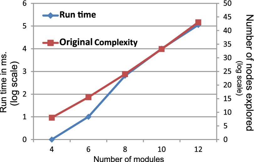
In the first set of experiments, we analyzed the effect of the main concept of our algorithm, i.e., finding the best coalition structure possible from the CSG. As shown in Table 2, for $4 \leq | A | \leq 12$ , our algorithm was able to do a search in the space of all coalition structures and find the optimal coalition structure for all values of $| A |$ . For higher values of $| A |$ the exhaustive search (complexity $O (| A |^{| A |})$ ) becomes prohibitive. The value of $l_{n_{max}}$ is fixed to 2 for this test. These data show that our algorithm takes a fraction of a second to find the best coalition structure. With 6 modules, the algorithm takes only 2 milliseconds, whereas for 12 modules, the run time of the algorithm is 33 milliseconds. When $l_{n_{max}}$ is fixed to 3, run time of the algorithm with 12 modules increased to 667 ms. Figure 10 shows how actual space complexity for our algorithm and the run time to explore the nodes change with the number of modules. It is evident from this figure that even though space complexity is increasing exponentially with increasing number of modules, our algorithm maintains the run time within a reasonable value and finds the optimal coalition structure. This also shows that our algorithm scales well with number of modules.

Fig. 10.

Comparison of run time of the $bottomUpCSGSearch$ algorithm and actual space complexity against the number of modules.

5.2.2. Comparisons with existing algorithms

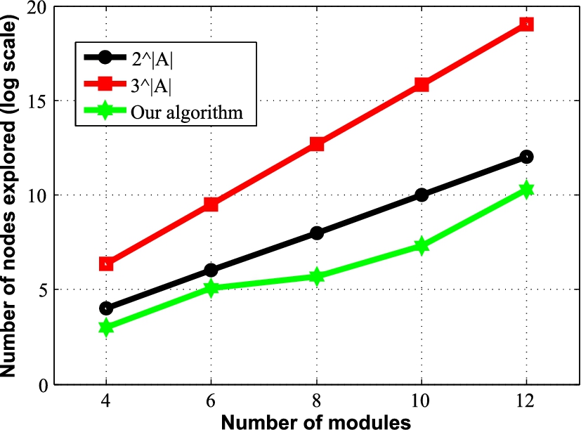
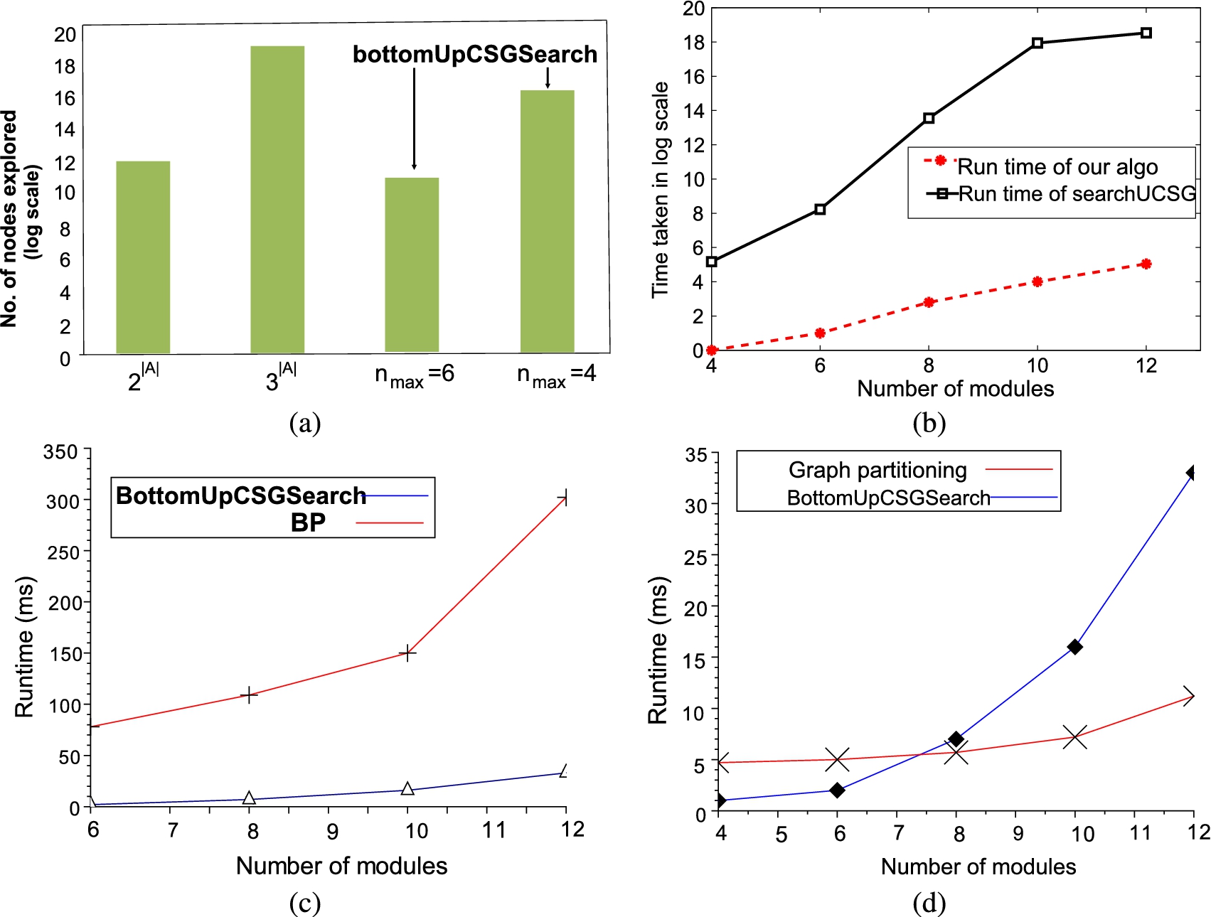
Figure 11 shows the comparison between the number of nodes explored by our proposed algorithm with the existing coalition structure search algorithms proposed in [26] and [23]. These algorithms are anytime in nature and have worst case time complexities $O (3^{| A |})$ and $O (2^{| A |})$ respectively. As these algorithms do not necessarily support size-constrained value functions, the numbers of nodes explored in the CSG by them are higher than our proposed algorithm. The graph is shown on a logarithmic ( ${log}_{2}$ ) scale. The value of $n_{max}$ is set to 2 for $| A | = 4$ modules, 4 for $| A | = 6$ modules and 6 for $| A | ⩾ 8$ modules. This graph shows that our algorithm is able to prune more of the unpromising search space than the other two algorithms and consequently its time and space complexities also reduce.

Fig. 11.

Comparison of number of nodes explored by different existing coalition structure generation algorithm and the proposed $bottomUpCSGSearch$ algorithm.

In our next set of experiments, we compared the number of nodes generated by our algorithm for 12 modules against previously studied algorithms for coalition structure generation in [26] and [23]; $n_{max}$ is varied between 4 and 6. Figure 12a shows the number of nodes generated in all the algorithms on a logarithmic ( ${log}_{2}$ ) scale. As can be seen, our algorithm explores $2^{3}$ times fewer nodes when $n_{max} = 4$ and $2^{8}$ times fewer nodes when $n_{max} = 6$ , than the algorithm in [26]. It also explores 2 times fewer nodes in the case of $n_{max} = 6$ than the algorithm in [23]. This illustrates that using a CSG search algorithm for the unconstrained coalition formation problem can become inefficient for the coalition size-constrained coalition formation problem, as the number of agents increases. It is also understood that the algorithm proposed in this paper is a function of $n_{max}$ rather than of $| A |$ .

Fig. 12.

a) Comparison of number of nodes generated with existing algorithms – for 12 modules, with varying $n_{max}$ ; b) Run time comparison with $searchUCSG$ algorithm; c) Run time comparison with $graphPartitioning$ algorithm; d) Run time comparison with $BP$ algorithm.

Next we have compared the run time of our algorithm with existing algorithms where coalition structure search algorithms have been used for configuration generation in ModRED [3]. The first algorithm we compared with is searchUCSG. Figure 12b shows the comparison of our algorithm’s run time with searchUCSG [10], where the authors proposed a top-down, heuristics-based search algorithm to search the CSG. It shows that for 12 agents, the $searchUCSG$ algorithm took 3.81 × 10⁵ milliseconds whereas our proposed bottomUpCSGSearch algorithm took only 33 milliseconds to find the optimal solution – a run time improvement in the order of $10^{4} ms$ . The main reason behind this improvement in time is that we start the search from the bottom of the CSG and therefore we reach the level $l_{n_{max}}$ , where nodes with maximum number of $n_{max}$ -sized coalitions are stored, faster than the searchUCSG algorithm.

Our next comparison was done with the BP algorithm, where the coalition size is constrained by $n_{max}$ , using a hard constraint, i.e., no coalition with size more than $n_{max}$ was generated. The BP algorithm partitions the coalitions of different sizes into multiple blocks and searches through these blocks to form the coalition structures. Our bottomUpCSGSearch algorithm takes less run time than the BP algorithm (Fig. 12c). For example, by using the BP algorithm, for 6 and 12 modules, the run times are 78 and 302 milliseconds respectively, whereas for the same number of modules bottomUpCSGSearch takes 2 and 33 milliseconds run time respectively – an improvement of almost 10 times.

Lastly, we compared bottomUpCSGSearch with a graph partitioning algorithm [6]. This algorithm restricts the problem to a weighted graph where coalition utilities are calculated by summing pairwise utilities (edge weights), making it a polynomial problem. On the other hand, our algorithm tries to deal with the original NP-hard problem without any assumption or relaxation. This comparison is shown in Fig. 12d. Being a NP-hard problem, our algorithm performs comparably against the polynomial-relaxed graph partitioning algorithm – for 12 modules, our bottomUpCSGSearch algorithm takes 33 milliseconds while the graph partitioning algorithm takes 11 milliseconds – only 3 times worse than a polynomial solution.

Fig. 13.

(a)–(c) Exploring the anytimeness nature of the proposed $bottomUpCSGSearch$ algorithm – for 8, 10 and 12 modules; d) Effect of changing $n_{max}$ on number of explored nodes – for 10 modules.

5.2.3. Empirical evaluation of the anytimeness property

In the next set of experiments, we have tested the anytimeness property of our proposed algorithm. Figures 13a–c show the anytimeness nature of our algorithm, for 8, 10 and 12 modules respectively. The x-axis denotes the percentage of total time elapsed and the y-axis denotes the percentage of the best utility found in that particular time-step. For these tests, $l_{n_{max}}$ is set to 2. As can be seen from these figures, for 8 modules (Fig. 13a), the best coalition structure is found in about 40% of the total time, whereas for 12 modules (Fig. 13c), the best coalition structure is found in about 10% of the total time. One should note that as the total run times of the algorithm for 8, 10 and 12 modules are not the same, 10% of the total time for 12 modules is not necessarily less clock time than 40% of the total time for 8 modules.

5.2.4. Experiments with $n_{max}$

For the next set of experiments, we varied $n_{max}$ through 4, 5, 6 while keeping $| A |$ fixed at 10 (Fig. 13d) and as can be seen, compared to the total number of nodes possible in those levels, we were able to restrict the number of explored nodes within a polynomial bound and still achieved optimal utility every time. Also this figure shows that for $n_{max} = 4$ , more nodes are explored than when $n_{max} = 5$ or 6. When $n_{max} = 4$ , then $l_{n_{max}} = 3$ , whereas when $n_{max} = 5$ or 6, then $l_{n_{max}} = 2$ , instead of 3. So, we can see than when $n_{max}$ is set to 4, then more need to be explored in order to reach the best level. On the other hand, when $n_{max}$ is set to 5 or 6, to reach the best level, fewer nodes are explored. This is why our algorithm’s complexity depends on both $| A |$ and $n_{max}$ – more specifically on the value of $l_{n_{max}} (= ⌊ \frac{| A |}{n_{max}} ⌋)$ .

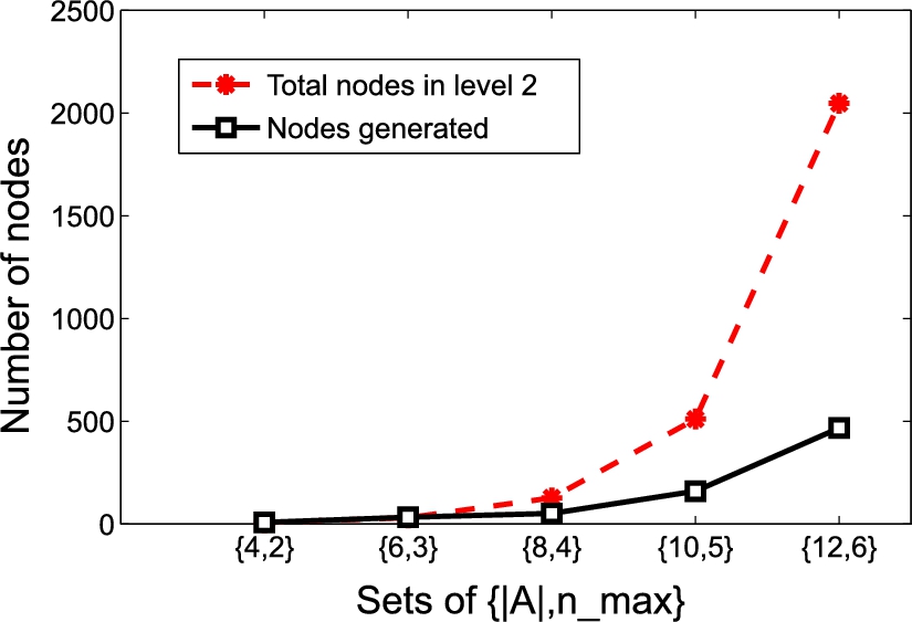
We have also experimented with the effect of the set of ${| A |, n_{max}}$ on the number of explored nodes in the CSG. We experimented with different values of $| A |$ and $n_{max}$ while maintaining $l_{n_{max}}$ at 2. The different combinations of $| A |$ and $n_{max}$ that were used are: ${4, 2}$ , ${6, 3}$ , ${8, 4}$ , ${10, 5}$ and ${12, 6}$ . From Fig. 14, it is evident that though the total number of nodes in level 2 increased exponentially, still our algorithm was able to keep the number of nodes generated polynomial with respect to the increasing values of $l_{n_{max}}$ , while finding the optimal coalition structure.

Fig. 14.

Comparison of total number of nodes in $l_{n_{max}} = 2$ vs. no. of nodes generated.

Fig. 15.

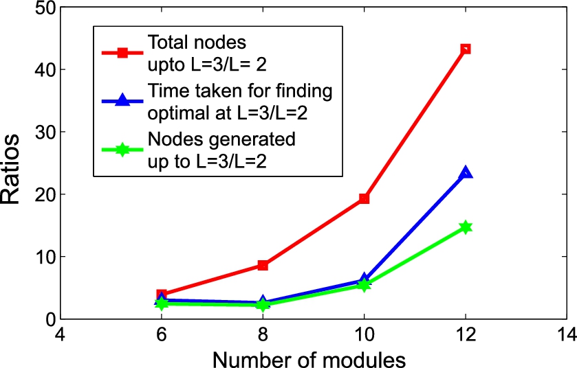
Ratios between total number of nodes, number of nodes generated and time taken to find optimal for $l_{n_{max}} = 2$ and 3.

For the next set of experiments, we took the ratios between the total number of nodes up to level 3 and level 2, between the number of nodes explored in those levels and also between the total time taken for exploring nodes in those two levels. This is shown in Fig. 15, which shows that the ratio of total number of nodes possible in level 2 and 3 is exponentially increasing. But in case of our algorithm, the ratio of total number of nodes explored in those levels increased in a polynomial fashion. Therefore the graph for the ratio of time taken for exploring nodes in those two levels did not increase exponentially.

6. Conclusion and future work

We have proposed a dynamic partitioning technique for configuration generation in modular robots. This paper models the problem as a CSG search problem for finding the best coalition structure and intelligently generates, searches and prunes nodes in the CSG. We have also provided analysis on worst case guarantees that our proposed algorithm provides. We have shown that our algorithm is optimal, anytime and complete, and also provided a complexity analysis for the algorithm. We have empirically shown that our algorithm scales well with the number of modules. We have compared the performance of our algorithm with existing algorithms for similar problems and empirically shown that the proposed bottomUpCSGSearch algorithm performs better than most of the existing solutions, in terms of number of nodes generated and also time taken to execute the algorithm. This paper deals with a very unique problem in modular robotics – partitioning a set of modules (robots) for forming the best utility teams (configurations). Our proposed algorithm is one of the very first approaches to solve this problem. We have experimented with different values of $n_{max}$ , maximum size that an MSR can have, and shown that even with different $n_{max}$ values, our algorithm scales well.

As future work, we are investigating a structured way to learn the value function and the parameter $n_{max}$ based on modules’ past performances, their abilities and task types. In the future, we will incorporate techniques to learn the optimal value of $n_{max}$ in different environmental situations and terrain types. We are also investigating coalition formation algorithms that can be executed quickly within the time and space constraints of physical ModRED hardware. Also we are developing an algorithm for forming any given shape from the initial singletons and configurations, using a position selection based approach. Finally, we are working on implementing this algorithm on physical ModRED modules.

Footnotes

Acknowledgement

This research has been supported by NASA grant no. NNX11AM14A as part of the ModRED project.

References

[1]

G.E.

Andrews, The Theory of Partitions, Number 2, Cambridge University Press, 1998.

[2]

Baca,

Dasgupta,

S.G.M.

Hossain and

Nelson, Modular robot locomotion based on a distributed fuzzy controller: The combination of modred’s basic module motions, in: 2013 IEEE/RSJ International Conference on Intelligent Robots and Systems (IROS), IEEE, 2013, pp. 4302–4307.

[3]

Baca,

S.G.M.

Hossain,

Dasgupta,

C.A.

Nelson and

Dutta, Modred: Hardware design and reconfiguration planning for a high dexterity modular self-reconfigurable robot for extra-terrestrial exploration, Robotics and Autonomous Systems 62(7) (2014), 1002–1015.

[4]

Chirikjian,

Pamecha and

Ebert-Uphoff, Evaluating efficiency of self-reconfiguration in a class of modular robots, Journal of Robotic Systems 13(5) (1996), 317–338.

[5]

K.D.

Chu,

S.G.M.

Hossain and

C.A.

Nelson, Design of a four-dof modular self-reconfigurable robot with novel gaits, in: ASME 2011 International Design Engineering Technical Conferences and Computers and Information in Engineering Conference, American Society of Mechanical Engineers, 2011, pp. 747–754.

[6]

Dasgupta,

Ufimtsev,

Nelson and

S.G.M.

Hossain, Dynamic reconfiguration in modular robots using graph partitioning-based coalitions, in: Proc. of the 11th International Conference on Autonomous Agents and Multiagent Systems, Vol. 1, International Foundation for Autonomous Agents and Multiagent Systems, 2012, pp. 121–128.

[7]

De Rosa,

Goldstein,

Lee,

Campbell and

Pillai, Scalable shape sculpturing via hole motions, in: IEEE Intlernational Conference on Robotics and Automation, Orlando, FL, 2006, pp. 1462–1468.

[8]

Dutta,

Dasgupta,

Baca and

Nelson, A block partitioning algorithm for modular robot reconfiguration under uncertainty, in: 2013 European Conference on Mobile Robots (ECMR), IEEE, 2013, pp. 255–260.

[9]

Dutta,

Dasgupta,

Baca and

Nelson, A bottom-up search algorithm for dynamic reformation of agent coalitions under coalition size constraints, in: 2013 IEEE/WIC/ACM International Joint Conferences on Web Intelligence (WI) and Intelligent Agent Technologies (IAT), Vol. 2, IEEE, 2013, pp. 329–336.

10.

[10]

Dutta,

Dasgupta,

Baca and

Nelson, Searchucsg: A fast coalition structure search algorithm for modular robot reconfiguration under uncertainty, Robotica 32(2) (2014), 225–244.

11.

[11]

Fitch and

Butler, Million module march: Scalable locomotion for large self-reconfiguring robots, The International Journal of Robotics Research 27(3–4) (2008), 331–343.

12.

[12]

Grabowski,

L.E.

Navarro-Serment,

C.J.J.

Paredis and

P.K.

Khosla, Heterogeneous teams of modular robots for mapping and exploration, Autonomous Robots 8(3) (2000), 293–308.

13.

[13]

S.G.M.

Hossain,

C.A.

Nelson,

K.D.

Chu and

Dasgupta, Kinematics and interfacing of modred: A self-healing capable, 4dof modular self-reconfigurable robot, Journal of Mechanisms and Robotics 6(4) (2014), 041017.

14.

[14]

S.G.M.

Hossain,

C.A.

Nelson and

Dasgupta, Rogensid: A rotary plate genderless single-sided docking mechanism for modular self-reconfigurable robots, in: ASME 2013 International Design Engineering Technical Conferences and Computers and Information in Engineering Conference, American Society of Mechanical Engineers, 2013, p. V06BT07A011.

15.

[15]

Hou and

W.-M.

Shen, Distributed, dynamic, and autonomous reconfiguration planning for chain-type self-reconfigurable robots, in: IEEE International Conference on Robotics and Automation, 2008, ICRA 2008, IEEE, 2008, pp. 3135–3140.

16.

[16]

M.W.

Jorgensen,

E.H.

Ostergaard and

H.H.

Lund, Modular atron: Modules for a self-reconfigurable robot, in: Proc. of the 2004 IEEE/RSJ International Conference on Intelligent Robots and Systems (IROS 2004), Vol. 2, IEEE, 2004, pp. 2068–2073.

17.

[17]

Kurokawa,

Tomita,

Kamimura,

Kokaji,

Hasuo and

Murata, Distributed self-reconfiguration of m-tran iii modular robotic system, The International Journal of Robotics Research 27(3–4) (2008), 373–386.

18.

[18]

M.D.M.

Kutzer,

M.S.

Moses,

C.Y.

Brown,

D.H.

Scheidt,

G.S.

Chirikjian and

Armand, Design of a new independently-mobile reconfigurable modular robot, in: 2010 IEEE International Conference on Robotics and Automation (ICRA), IEEE, 2010, pp. 2758–2764.

19.

[19]

Lyder,

R.F.

Mendoza Garcia and

Stoy, Mechanical design of odin, an extendable heterogeneous deformable modular robot, in: IEEE/RSJ International Conference on Intelligent Robots and Systems, 2008, IROS 2008, IEEE, 2008, pp. 883–888.

20.

[20]

Meier, Variance of a weighted mean, Biometrics 9(1) (1953), 59–73.

21.

[21]

R.B.

Myerson, Game Theory: Analysis of Conflict, Harvard University Press, Cambridge, Massachusetts, 1997.

22.

[22]

Rahwan and

N.R.

Jennings, An improved dynamic programming algorithm for coalition structure generation, in: Proc. of the 7th International Joint Conference on Autonomous Agents and Multiagent Systems, 2008, pp. 1417–1420.

23.

[23]

Rahwan,

S.D.

Ramchurn,

N.R.

Jennings and

Giovannucci, An anytime algorithm for optimal coalition structure generation, Journal of Artificial Intelligence Research 34 (2009), 521–567, 2012.06.16.

24.

[24]

M.H.

Rothkopf,

Pekeč and

R.M.

Harstad, Computationally manageable combinational auctions, Management Science 44(8) (1998), 1131–1147.

25.

[25]

S.J.

Russell,

Norvig,

J.F.

Canny,

J.M.

Malik and

D.D.

Edwards, Artificial Intelligence: A Modern Approach, Prentice Hall, Englewood Cliffs, 2009.

26.

[26]

Sandholm,

Larson,

Andersson,

Shehory and

Tohmé, Coalition structure generation with worst case guarantees, Artificial Intelligence 111(1–2) (1999), 209–238.

27.

[27]

Sen and

P.S.

Dutta, Searching for optimal coalition structures, in: Proc. of the 4th International Conference on MultiAgent Systems, 2000, IEEE, 2000, pp. 287–292.

28.

[28]

Shehory and

Kraus, Methods for task allocation via agent coalition formation, Artificial Intelligence 101(1) (1998), 165–200.

29.

[29]

Shoham and

Leyton-Brown, Multiagent Systems: Algorithmic, Game-Theoretic, and Logical Foundations, Cambridge University Press, 2009.

30.

[30]

Stoy,

Brandt and

D.J.

Christensen, Self-Reconfigurable Robots: An Introduction, The MIT Press, 2010.

31.

[31]

S.H.

Wilf, Generatingfunctionology, Elsevier, 2013.

32.

[32]

Yim,

W.-M.

Shen,

Salemi,

Rus,

Moll,

Lipson,

Klavins and

G.S.

Chirikjian, Modular self-reconfigurable robot systems [grand challenges of robotics], IEEE Robotics & Automation Magazine 14(1) (2007), 43–52.

33.

[33]

Yoshida,

Matura,

Kamimura,

Tomita,

Kurokawa and

Kokaji, A self-reconfigurable modular robot: Reconfiguration planning and experiments, The International Journal of Robotics Research 21(10–11) (2002), 903–915.

34.

[34]

Zilberstein, Using anytime algorithms in intelligent systems, AI magazine 17(3) (1996), 73.

A bottom-up search algorithm for size-constrained partitioning of modules to generate configurations in modular robots

Abstract

Keywords

1. Introduction

2 In this paper, we assume that initially all the modules are singletons.

5.1. Experimental setup

5.2.1. Solution quality and run time

5.2.4. Experiments with n max

Footnotes

Acknowledgement

References

²
In this paper, we assume that initially all the modules are singletons.

5.2.4. Experiments with $n_{max}$