Modified convolutional neural network for lung cancer detection: Improved cat swarm-based optimal training

Abstract

Lung cancer is the most lethal and severe illness in existence. However, lung cancer patients may live longer if they receive early detection and treatment. In the medical field, the best imaging technique is CT scan imaging as it is more complex for doctors to identify cancer and interpret from CT scan images. Consequently, the computer-aided diagnosis (CAD) is more useful for doctors to find out cancerous nodules. To identify lung cancer, a number of CAD techniques utilising machine learning (ML) and image processing are used nowadays. The goal of this study is to present a novel method for detecting lung cancer that entails four main steps: (i) Pre-processing, (ii) Segmentation, (iii) Feature extraction, and (iv) Classification. ”The input image is first put through a pre-processing step in which the CLAHE model is used to pre-process the image. The segmentation phase of the pre-processed images is then initiated, and it makes use of a modified Level set segmentation method. The retrieved features from the segmented images include statistical features, colour features, and texture features (GLCM, GLRM, and LBP). The Layer Fused Conventional Neural Network (LF-CNN) is then utilised to classify these features in the end. Particularly, layer-wise modification is carried out, and along with that, the LF-CNN is trained by the Modified Cat swarm Optimization (MCSO) Algorithm via selecting optimal weights. The accepted scheme is then compared to the current models in terms of several metrics, including recall, FNR, MCC, FDR, Threat score, FPR, precision, FOR, accuracy, specificity, NPV, FMS, and sensitivity.

Keywords

Lung cancer detection pre-processing segmentation feature extraction optimization

Nomenclature

mRFCN

multidimensional Region-based Fully Convolutional Network

Linear Regression

Computed Tomography

LDA

Linear Discriminant Analysis

CAD

Computer-Aided Design

Deep Learning

kNN

k-Nearest Neighbor

CNN

Convolutional Neural Networks

Decision Tree

CADe

Computer-Aided Detection

SEREX

Serological Analysis of Recombinant cDNA Expression Libraries

PDF

Probability Density Function

ELISA

Enzyme-Linked Immune Sorbent Assay

IPCT

Improved Profuse Clustering Technique

SVM

Support Vector Machine

IDNN

Improved Deep Neural Network

TAAs

Tumor-Associated Antigens

CIA

Cancer Imaging Archive

ROI

Region of Interest

CLAHE

Contrast Limited Adaptive Histogram Equalization

PSSM

Position-Sensitive Score Maps

mLRPN

Multi-Layer Fusion Region Proposal Network

WHO

World Health Organization

AUC

Area Under Curve

CLHE

Contrast Limited Histogram Equalization

DITNN

Deep Learning with Instantaneously Trained Neural Networks

CDF

Cumulative Density Function

SDF

Signed Distance Function

MCSO

Modified Cat Swarm Optimization

GLRM

Grey Level Runlength Matrix

LBP

Local Binary Pattern

LF-CNN

Layer Fused Conventional Neural Network

GLCM

Grey Level Co-ocurrence Matrix

SMP

Seeking Memory Pool

FDR

False Discovery Rate

CDC

Counts of Dimension to Change

SPC

Self-Position Considering

FDR

False Discovery Rate

FMS

F-Measure

MCC

Matthews Correlation Coefficient

FPR

False Positive Rate

WOA

Whale Optimization Algorithm

DBN

Deep Belief Network

SRD

Seeking Range of the selected Dimension

Mixture Ratio

FNR

False Negative Rate

NPV

Net Predictive Value

MFO

Moth Flame Optimization

FOR

False Omission Rate

1. Introduction

The leading cause of death all over the world during the year 2018 is 9.6 million, as per the report of WHO [21,24]. Moreover, lung cancer causes the uppermost mortality rates. The clinical reports indicated that early lung cancer treatment would increase the survival rate [30]. Consequently, the early detection of lung cancer is investigated extensively around the world by different research groups and medical corporations. However, it is more complex because it arises and illustrates symptoms only at the final stage [55]. Still, it is believed that the probability and mortality rate are lowered through the early detection and treatment of the disease. Nowadays, lung cancer is signified as the post deadliest disease, which poses a great threat to humans due to the spreading of smoke, the high rates of air pollution, and the more complex treatment [6]. Therefore, the early detection of lung cancer in the medical field is a major concern of scientists. The most excellent imaging approach is reliable for lung cancer diagnosis using CT images as it discloses every unsuspected and suspected lung nodules [19].

CT images outperformed traditional radiography for screening the lungs as it produces detailed high-resolution images and showed the early-stage lesion that is too small to be detected through traditional X-ray [31]. The growing body of medical data is also beneficial for healthcare practitioners who want to raise the standard of care [48]. Many governments now consider improving individualized healthcare to be one of their major responsibilities [33]. In addition, CT is widely used for detecting different lung diseases like pulmonary edema, pneumonia, lung cancer, and pneumoconiosis [50]. It is regarded as the most challenging task by radiologists owing to the large amount of information generated through the CT scan [14]. Consequently, CAD systems are required for helping radiologists during the evaluation and analysis of CT scans. Furthermore, the CAD system analyzes the medical images in different steps such as preprocessing step for enhancing the image quality and noise reduction, and then the segmentation step for differentiating the ROI in the image [4,28]. Following the segmentation procedure, several features such as textural, statistical, and geometrical attributes are extracted. The evaluation or classification step is performed for evaluating and diagnosing the ROI based on extracted features [43]. Several models have been employed in previous research to construct prediction models to improve forecast accuracy [17].

CAD systems are divided into 2 groups deep-learnable and classical systems. Further, the classical CADe systems are started usually through the extracted lung regions, and then it uses the shape, texture features, and intensity taken from the lung regions for detecting lung cancer [5,51]. Additionally, deep-learnable CADe algorithms are used to address the shortcomings of lung cancer diagnosis. The DL techniques [16,39] and CNN [7,10,40,46] are the most important approaches used for the analysis of medical images and in computer vision applications. The DL techniques [37,38,47] are used for extracting the data features efficiently that determine the current problem through many layers-networks [9,53]. One of the most successful DL medical image analyzers is the CNNs [18]. Optimization difficulties present a challenge in terms of minimizing or maximizing an objective function [27]. Even though the innovations in pulmonary cancer are unsteady and slow based on survival rate; DL approaches [13,15] provides promising outcomes and thru these detection systems, the lung cancer death rate is declined.

The following list of the model’s main contributions:

Suggests using a CNN layer that has been fused for the final prediction of lung cancer images.

Exposes the Modified Cat Swarm Optimization (MCSO) Method for determining the best weights for training a LF-CNN model.

Section 2 of this essay presents a review of lung cancer detection. Section 3 gives an overview of the intended work. Pre-processing via CLAHE model and segmentation process via modified level set algorithm is presented by Section 4. The process of extracting texture, statistical, and colour information is described in Section 5. The categorisation of lung cancer is shown in Section 6 using a modified cat swarm optimisation approach and a CNN that has been tuned for training. The outcome and discussion are described in Section 7. Section 8 completes the essay at last.

2. Literature review

2.1. Related works

In 2019, Sori et al. [45] has examined the multi-path CNN for the detection of lung cancer. Moreover, the deep CNN architecture was implemented that differs from the conventionally used computer vision framework for solving these issues. Moreover, the suspicious nodule was produced along with the U-Net’s modified version and then the produced nodules act as the input data in the adopted model. Further, the adopted scheme was the multi-path CNN that exploited both the global contextual features and the local features to detect lung cancer automatically. The retraining phase system was implemented, which permits tackling the issues oriented to image labels imbalance. Furthermore, when compared to the conventional methods, the experimental results of both the standard type have produced improved detection outcomes.

In 2019, Mesut et al. [49] have developed the low redundancy high relevance feature selection approach on chest CT images with CNNs for the detection of lung cancer. Furthermore, lung cancer identification was recognized by VGG-16 deep learning, AlexNet, and LeNet schemes. Moreover, the classification and the feature extraction process were performed by the CNNs. Separate from either the final fully-connected layer of this method, the features obtained were used as the inputs to LDA, CNN, LR, SVM, softmax classifiers, and DT. An image augmentation approaches like horizontal turning, zooming, filling, and cutting was applied during the training for increasing the success rate of classification. Last but not least, the simulation outcomes of the accepted model have demonstrated higher classification accuracy, higher sensitivity, higher specificity, time consumed, and reduced memory usage.

In 2020, Shakeel et al. [41] have designed a novel machine learning technique and optimized image processing for predicting lung cancer. The collected images were determined by applying the multilevel brightness-preserving model that removes the noise, maximizes the quality of the lung image, and examines each pixel effectively. The affected region was segmented through an IDNN which segments the region based on the network layers and extracts different features from the noise-removed lung CT image. Furthermore, the simulation outcomes of the suggested model have increased F-score for predicting lung cancer and decreased mean absolute error, logarithmic loss, and precision.

In 2020, Masood et al. [23] has implemented an improved mRFCN based automated decision support scheme for lung nodule classification and detection. Moreover, the mRFCN was used for feature extraction with the new mLRPN and PSSM as a helping hand of image classification. Further, the median intensity projection was applied from CT scans and deconvolutional layer to leverage 3D information that was introduced for adopting the proposed mLRPN to select the potential ROI. The model that has been provided has generated positive experimental results with a more promising detection performance than other existing methods with respect to sensitivity and classification accuracy.

In 2020, Zhan et al. [54] has suggested a new application in lung cancer diagnosis based on conformal prediction. Moreover, the nonconformity measurement was performed on the basics of KNN. High accuracy of the proposed model has been attained through the conformal predictors of 1NN and 3NN respectively in the offline prediction that outperforms the simple KNN predictors. In addition, the conformal predictors provided more confidence and credibility information for predicting the patient’s severity. Further, the experimental results of the adopted approach have proven higher overall sensitivity, maximum prediction accuracy, and better credibility.

In 2021, Feng et al. [44] has introduced the “denoising first two-path CNN” (i.e.), DFD-Net for addressing its complexity. In addition, the implemented model consists of detection part and denoising in an end-to-end manner. Moreover, the “residual learning denoising approach (i.e.) DR-Net” was utilized during the preprocessing stage for removing the noises. Furthermore, a two-path CNN has taken the denoised image as input through DR-Net for lung cancer detection. A retraining technique was proposed for overcoming the problems linked to the imbalance of image labels. And last, the model’s simulation results affords the receptive field size effect balance, more representative features, reduce noise in an image, and effortlessly flexibility to the discrepancy between the size and shape of the nodule.

In 2019, Mohamed et al. [42] examined the improvement in the quality of lung image and lung cancer diagnosis by lowering the misclassification. The DITNN and the IPCT approach were used for predicting lung cancer through lung CT images. Furthermore, the CIA dataset, which consists of 5043 DICOM file images divided into 2043 test images and 3000 training images, was used to gather the lung CT scans. Finally, the suggested model successfully predicts cancer with improved accuracy and a lower classification error.

In 2019, Lu et al. [32] have suggested the TAAs identification and their equivalent autoantibodies in LC that expanded the vision of cancer immunity. The objective of the proposed model has screened the new TAAs from the healthy population to distinguish LC. Moreover, the Oncomine database was utilized for identifying the potential genes in cancer progression and 35 genes encrypt LC-associated TAAs was recognized by SEREX. The ELISA in sera was used for testing the Auto-antibodies in the verification set and validation set from 1379 participants. Ultimately, the accepted model’s output has a high AUC, the highest sensitivity, and the highest specificity.

In 2021, Priya et al. [34] have deployed a learning rate-modified convolutional neural network algorithm based on BAT optimization presented in this research. Additionally, the input picture is deconstructed with assistance from the Discrete Wavelet Transform to enhance the proposed classification performance (DWT). With, the image is divided into four subbands; in this instance, the Low (LL) band image was taken into consideration. After that, two sets of segmentation results are split into training and testing groups. The publicly accessible LIDC-IDRI dataset was used to validate the proposed approach. A convolutional neural network is used to study them, and a quickly trained neural network for LC prediction is also applied. In the end, a MATLAB tool is used to determine the system’s effectiveness.

In 2021 Xin et al. [22] have deployed a brand-new convolutional neural network. For greater network accuracy and optimal organization, the marine predator’s algorithm is also applied. Finally, the technique was fixed to RIDER dataset as well as outcomes were evaluated against those of a few pre-trained deep networks, includes CNN ResNet-18, GoogLeNet, AlexNet, and VGG-19. The end results showed that the proposed approach outperformed the compared strategies.

Table 1
Review on existing lung cancer detection schemes: features and challenges

Author [citation] Proposed method Features Challenges

Sori et al. [45] Multi-path CNN model ✓More flexible The additional feature does not give any significant improvement in the results.

✓Better accuracy

✓Specificity is raised

✓Higher recall

Mesut et al. [49] CNN model ✓Higher classification accuracy The super pixel approach was not examined on this dataset.

✓Better sensitivity

✓Higher specificity

✓Time-consumption

✓Lower memory usage

Shakeel et al. [41] IDNN model ✓Maximum gets raised The selected method don’t have a single gradient function.

✓Higher specificity

✓Increased precision

✓Better Recall

✓Improved F1 score

Masood et al. [23] mRFCN based automated decision support system ✓High sensitivity Detection of some micronodules (i.e.), less than 3 mm in diameter was not focused.

✓The maximum low error rate

✓Higher classification accuracy

Zhan et al. [54] KNN approach ✓Higher overall sensitivity Different approaches to nonconformity measurement in conformal predictions were not applied.

✓Maximum prediction accuracy

✓Better credibility

Feng et al. [44] DFD-Net model ✓Low noise Equal or higher accuracy number having denoised images was not obtained in the proposed approach.

✓Easily adaptable

✓High specificity

✓Better Recall

✓Maximum accuracy

Mohamed et al. [42] IPCT and DITNN approach ✓Better accuracy The greater or same accuracy value was not obtained with the denoised images in the proposed approach.

✓Minimum classification error

Lu et al. [32] ELISA test ✓Better AUC Differences in autoantibodies were not observed in the different cancers.

✓Maximum sensitivity

✓Higher specificity

Priya et al. [34] BAT Optimization ✓The classification accuracy is improved The processing is very slow.

✓The method is very simple

Xin et al. [22] Brand-new CNN ✓The performance efficiency is improved. The speed is reduced in the real-time application

✓The space is saved.

Author [citation]	Proposed method	Features	Challenges
Sori et al. [45]	Multi-path CNN model	✓More flexible	The additional feature does not give any significant improvement in the results.
✓Better accuracy
✓Specificity is raised
✓Higher recall
Mesut et al. [49]	CNN model	✓Higher classification accuracy	The super pixel approach was not examined on this dataset.
✓Better sensitivity
✓Higher specificity
✓Time-consumption
✓Lower memory usage
Shakeel et al. [41]	IDNN model	✓Maximum gets raised	The selected method don’t have a single gradient function.
✓Higher specificity
✓Increased precision
✓Better Recall
✓Improved F1 score
Masood et al. [23]	mRFCN based automated decision support system	✓High sensitivity	Detection of some micronodules (i.e.), less than 3 mm in diameter was not focused.
✓The maximum low error rate
✓Higher classification accuracy
Zhan et al. [54]	KNN approach	✓Higher overall sensitivity	Different approaches to nonconformity measurement in conformal predictions were not applied.
✓Maximum prediction accuracy
✓Better credibility
Feng et al. [44]	DFD-Net model	✓Low noise	Equal or higher accuracy number having denoised images was not obtained in the proposed approach.
✓Easily adaptable
✓High specificity
	✓Better Recall
	✓Maximum accuracy
Mohamed et al. [42]	IPCT and DITNN approach	✓Better accuracy	The greater or same accuracy value was not obtained with the denoised images in the proposed approach.
✓Minimum classification error
Lu et al. [32]	ELISA test	✓Better AUC	Differences in autoantibodies were not observed in the different cancers.
✓Maximum sensitivity
✓Higher specificity
Priya et al. [34]	BAT Optimization	✓The classification accuracy is improved	The processing is very slow.
✓The method is very simple
Xin et al. [22]	Brand-new CNN	✓The performance efficiency is improved.	The speed is reduced in the real-time application
✓The space is saved.

2.2. Review

The review of lung cancer detection is shown in Table 1. At first, the Multi-path CNN model was deployed in [45], which presents more flexibility, better accuracy, improved specificity, and higher recall; however, the additional feature does not give any significant improvement in the results. Wang-Scheme was exploited in [49] that offers higher classification accuracy, better sensitivity, higher specificity, time-consumption, and lower memory usage, but the super pixel approach was not examined in this dataset. Moreover, the IDNN model was deployed in [41] provide better recall, maximum accuracy, increased precision, improved F1 score, and higher specificity. Nevertheless, the adopted method does not have a single gradient function. Likewise, mRFCN based automated decision support system was exploited in [23], which offers high sensitivity, maximum low error rate, and higher classification accuracy. However, the detection of some micronodules (i.e.), less than 3 mm in diameter was not focused. KNN approach was exploited in [54] that have higher overall sensitivity, maximum prediction accuracy, and better credibility; however, different approaches of nonconformity measurement in conformal predictions were not applied. In addition, DFD – the net model was introduced in [44], which offers low noise, easily adaptable, high specificity, better recall, and maximum accuracy. However, the greater or same accuracy value was not obtained with the denoised images in the proposed approach. IPCT and DITNN approach was suggested in [42] that offers better accuracy, and minimum classification error. However, it does not require manually extracted features in the proposed model. Finally, the ELISA test was implemented in [32], which offers better AUC, maximum sensitivity, and higher specificity, but the differences in autoantibodies were not observed in the different cancers. Such limitations are taken into account to effectively diagnose lung cancer in the current work.

The likelihood of receiving effective therapy for lung disease will much depend on the timing of the diagnosis. Lung cancer can be diagnosed with the help of imaging, radiographs, & CT scans, in addition to biopsy, bronchoscopy, and evaluation of the breast mucosa. Numerous research have been done so far to identify and describe lung diseases. A specialist doctor may have difficulty distinguishing nodules from veins, wounds, etc. because of the removal of the lungs, the high number of radiographic images taken of them, and their complex and uneven structure. The fundamental principle is to employ the machine rather than leave the diagnosis to it since it improves the work’s sensitivity and lowers the rate of positive error. The processing time is high and it cannot diagnose the disease early. The prediction model is used in this study to address the shortcomings of the current methodology.

3. Overview of the proposed work: An architectural description

This research aims to present an unique method for detecting lung cancer that includes 4 critical stages: “(i) Pre-processing (ii) Segmentation (iii) Feature extraction and (iv) Classification”. At first, the input image is subjected to the CLAHE model to preprocess it. The segmentation phase is then applied to the previously processed images, where the image gets segmented using a modified Level set segmentation algorithm. From the segmented images, texture features (GLCM, GLRM, and LBP), statistical features (mean, mode, median, skewness, kurtosis, correlation, and entropy), and color features was get extracted. Additionally, the LF receives these qualities as input. -CNN for final classification. Particularly, the layer-wise modification is carried out, and along with that the MCSO Model is trained the LF-CNN by choosing the best weights. The recommended model’s overall structure is depicted in Fig. 1.

Fig. 1.

The general structure of the suggested model.

4. Preprocessing via the CLAHE model and segmentation by the modified level set algorithm

The input image ‘ $IM$ ’ is denoised and enhanced by the process of histogram equalization. Moreover, it is a well-known enhancement approach. The contrast and dynamic range of an image in histogram equalization are modified through varying the image, in which the histogram intensity has a required shape. Further, it is attained through the CDF as the mapping function. The intensity levels are changed, in which the histogram peaks are stretched and compressed in the troughs. If the digital image has M pixels dispersed indiscrete intensity levels $L I$ and $m_{l}$ indicates the number of pixels with $j_{l}$ intensity level and then the image PDF is determined as in Eq. (1). Furthermore, the CDF is given in Eq. (2). $\begin{array}{l} (1) & f_{j} (j_{l}) = \frac{m_{l}}{M} \\ (2) & F_{l} (j_{l}) = \sum_{i = 0}^{l} f_{j} (j_{i}) \end{array}$

4.1. CLAHE model

An adaptive contrast histogram equalization approach is known as the CLAHE, where it enhances the contrast of the image by applying it to tiny data regions known as tiles rather than the whole image. The resulting adjacent tiles are then stitched back flawlessly by the bilinear interpolation. Further, the contrasts in the homogeneous region are limited as it avoids noise amplification.

The CLAHE model applies the histogram equalization for every contextual region. The partition B is attained through the CLAHE [11] via 5 phases. The supplied image is first divided into identically sized, tiny blocks. The larger histograms is minimized by calculating the clip point in each block. The clip point estimation is determined as in Eq. (3). $\begin{matrix} (3) & β = \frac{{Px}_{i t}}{d r_{r l}} (1 + \frac{γ}{100} M s_{s o}) \end{matrix}$

In Eq. (3), β denotes the clip point, ${Px}_{i t}$ represents the pixel count in every section, $d r_{r l}$ denotes the dynamic range inside a specific block, $M s_{s o}$ refers to the higher slope, γ indicates the clip factor. So, ${IM}_{clahe}$ is the pre-processed image from the CLAHE model.

4.2. Modified levelset segmentation

The preprocessed image ${IM}_{clahe}$ is subjected to the segmentation process. The modified level set segmentation algorithm is used for the segmentation process. Here, the segmentation algorithm effectively segments the cancer regions premised on the velocities of surfaces having curvature-based velocities as well as moving curves. Here, the level team approach was extremely useful and influential. In the conventional level set segmentation the energy consumption and the consumption time is high. In the modified level set segmentation it overcomes the certain drawbacks. For image segmentation and parametric result comparison, it supports all sorts of image formats. The basic idea is to define the zero level set as the surfaces or curves of a superior dimensions hyper-surface. The fundamental thought is to characterize the surfaces or curves of a superior dimensional hyper-surface as the zero-level set. Moreover, the description of a smoothing function $ϕ (u, v, x)$ determines the surface whereas the definitions set $ϕ (u, v, x) = 0$ for the curves. Therefore, the curve evolution is changed into the 3D Level Set function evolution. Consider a $ϕ (u, v, x) = 0$ level set function, in which zero level set was related to the curve. The total surface is splitted into the curve’s internal and external regions. Further, the SDF on the surface is determined as in Eq. (4). $\begin{matrix} (4) & ϕ (u, v, x) = 0 = d \end{matrix}$

In Eq. (4), the d value is the minimum distance between d point on the curve and the surface. The entire curve’s evolutional process and its point are given in Eq. (5). The Level Set movement formula is determined in Eq. (6). $\begin{array}{l} (5) & ϕ (u, v, x) = 0 \\ (6) & ϕ_{t} + F | \nabla ϕ | = 0 \end{array}$

In Eq. (6), F indicates the speed function, in which the function is associated with the characteristics of the developing surface and image. The implementation F depends on the ideal value of zero and the image information on the target edge while applying it for segmentation. Due to its irrelevancy and stability with topology, the Level set method displayed a large advantage for solving the issues of corner point production, combing and curve breaking, etc. Consequently, it is used in a wide range. Moreover, it is required to remain the developing level set function near to signed distance function while implementing the level set method.

The energy function includes an external and an internal energy term, correspondingly. The external energy term $ε (ϕ)$ constrains the zero level set motion to the required image features including the object, while the boundaries internal energy term $Q (ϕ)$ determines the level set function deviation from the signed distance function. And resultant evolution is the gradient flow of the level set function that decreases the overall functional energy. Moreover, the energy function is given in Eq. (7). $\begin{matrix} (7) & \begin{matrix} EN (ϕ) & = μ Q (ϕ) + ε_{h, λ, g} (ϕ) \\ = μ \int_{Ω} \frac{1}{2} {(| \nabla ϕ | - 1)}^{2} d x d y + λ \int_{Ω} h δ (ϕ) | \nabla ϕ | d x d y + g \int_{Ω} h G (ϕ) d x d y \end{matrix} \end{matrix}$

In Eq. (7), $μ > 0$ refers to the parameter control of the penalizing effect with the ϕ deviation from an SDF, and h represents the function of edge indicator as given in Eq. (8). $\begin{matrix} (8) & h = \frac{1}{1 + | \nabla H_{σ} * I |^{2}} \end{matrix}$

In Eq. (8), $H_{σ}$ denotes the Gaussian kernel with σ SD, and I indicates an image. The SDF should satisfy the desirable property of $| \nabla ϕ | = 1$ . So, $G (ϕ)$ reflected the deviation among the SDF and level set function.

Modified levelset: The $φ_{o} (y, z)$ of the modified levelset is determined as in Eq. (9). $\begin{matrix} (9) & φ_{o} (y, z) = - 4 κ (0.3 - [0.6 (D_{1} + D_{2})]) \end{matrix}$

In Eq. (9), $D_{1}$ and $D_{2}$ indicates the initial contour results attained from FCM and k-means. κ refers to an invariable associated to disaco function. $\begin{matrix} (10) & δ_{EN} (w) = \{\begin{matrix} 0 & | w | > κ \\ \frac{1}{2 κ} [1 + cos (\frac{π w}{κ})] & | w | ⩽ κ \end{matrix} \end{matrix}$

The length $l s$ and area α are estimated using Eq. (11) and Eq. (12). $\begin{array}{l} (11) & l s = \int_{I} δ (φ_{o}) d y d z \\ (12) & α = \int_{I} P (φ_{o}) d y d z \end{array}$

Where $P (φ_{o})$ refers to the heavy side function and this was determined in Eq. (13). $\begin{array}{l} (13) & P (φ_{o}) = \{\begin{matrix} 1 & φ_{o} ⩾ 0 \\ 0 & φ_{o} < 0 \end{matrix} \end{array}$

Where, $μ = 0.2 l / α$ , $λ = 0.1 α / l$ , and $v = - 3 φ_{o} - 1$ . Thus, ${IM}_{seg}$ is the attained segmentation region of the image.

5. Feature extraction process: Texture, statistical, and color features

From the segmented regions, the texture features (GLCM, GLRM, LBP), statistical features (Mean, mode, median, entropy, correlation, skewness, and kurtosis), and color features are extracted.

5.1. Texture features

LBP The LBP [29] has computational simplicity and higher discriminative power. Additionally, the LBP operator labels each image pixel to decimal integers. During the labelling process, each imaging pixel is calculated with its surrounding pixels by subtracting the centre pixel value. Further, it encodes any negative values that are produced as 0, and it encodes the positive and 0 values as 1. The binary numbers created by concatenating all the binary digits in a clockwise motion starting from the top-left are known as LBP codes. All the many local representations that are combined to produce the global description are built using the texture descriptor. Additionally, based on the capacity to distinguish between these textured objects, the characteristics are retrieved. In Eq. (14), ${HS}_{p l}$ and ${HS}_{cl}$ denoted center pixel intensities as well as image center pixel by neighbor $p l$ , accordingly. The pixel’s LBP descriptor is displayed as $LBP (∙)$ and ${NE}_{P l}$ display neighbours total. And LBP descriptor function $F_{LBP (p l, cl)}$ was fed in Eq. (15). The resulting LBP characteristics are displayed as ${IM}_{LBP}$ . An LBP feature determines the size $1 \times 100$ by implementing the histogram. It is stated that the retrieved LBP-based feature is ${FE}_{LBP}$ . $\begin{array}{l} (14) & LBP ({HS}_{cl}) = \sum_{p l = 0}^{{NE}_{p l}} F_{LBP (p l, cl)} 2^{p l - 1} \\ (15) & F_{LBP (p l, cl)} = \{\begin{matrix} 1, & if {HS}_{p l} - {HS}_{cl} ⩾ 0 \\ 0, & otherwise \end{matrix}\} \end{array}$

GLCM features [ 35 ] The GLCM is an approach used to extract the 2nd order statistical texture features by the intensity values of statistical distributions that combines the image at various positions close to each other. Regardless of the number of task, an image’s statistics are divided into first, second, and high order categories. Higher order statistics are superior conceptually but are not developed due to computing complexity. Information about the surface’s internal structure and relationship to its surroundings is included in the texture features. Additionally, the texture-based capabilities of GLCM consist of “Energy, correlation, contrast, homogeneity, dissimilarity, ASM, GLCM-mean, GLCM-std, GLCM-max, GLCM-entropy, GLCM-skew, and GLCM-kurtosis”. The extracted 12 GLCM-based feature was displayed as ${FE}_{GLCM}$ and its size is $1 \times 12$ .

GLRM features [ 36 ] The texture is considered as a grey intensity pixel pattern in a certain direction from the reference pixels. Additionally, the GRLM is a matrices from which the texture analysis extracts the texture features. With the result of a comparable grey level for the scatter of pixels, GLRM calculates in which direction the pixels will move. The Run length is defined as the number of neighbouring pixels in a particular direction that have a similar grey intensity. The number of elements with an intensity in a certain direction is included in the 2D matrix of GLRM. Likewise, a texture-based GLRM features include “SRE, LRE, GLN, GLNN, RLN, RLNN, RP, LGLRE, HGLRE, SRLGLE, SRLHGLE, LRLGLE, LRHGLE, and GLV”. The extracted 14 GLRM features are denoted as ${FE}_{GLRM}$ and their size is $1 \times 14$ .

5.2. Statistical features

Along with the texture features, the statistical feature including mean, mode, median, entropy, kurtosis, skewness, & moment are also extracted. The size of statistical features is represented as $1 \times 7$ .

Mean (Average) [ 3 ] The process in which the sum of all values divided by the sum of some values is known to be the mean value. The mean was signified as $F S_{1}$ and it was manifested in Eq. (16). $\begin{matrix} (16) & F S_{1} = \bar{V} = \frac{1}{k s} \sum_{x = 1}^{k s} V \end{matrix}$

In Eq. (16), V represents the observed value, $k s$ shows sample size, and $\bar{V}$ displayed sample mean symbol.

Mode The “most frequent value in the dataset” is the mode. One of the most used “central tendency measures” (that is, used with “nominal data” that have entirely arbitrary class assignments) is this one. The mode was displayed as $F S_{2}$ .

Median The method used to arrange a dataset’s middle value in ascending order. When there are two middle elements in a dataset, the median is defined as the mean of the two middle values. A median was displayed as $F S_{3}$ . $\begin{matrix} (17) & F S_{3} = Median (V) = \{\begin{matrix} V (\frac{k s}{2}) & if k s is odd \\ \frac{V (\frac{k s - 1}{2}) + V (\frac{k s + 1}{2})}{2} & if k s is even \end{matrix} \end{matrix}$

In Eq. (17), $k s$ denotes the number of values and V indicates the ordered list of values in the dataset.

Entropy [ 2 ] Entropy is considered as the average level of a random variable with “information”, “surprise”, or “uncertainty” inherent to the possible variable’s resultant of the information theory. Sometimes, the information entropy was said to be Shannon entropy. Consider, V was discrete random variable having handed resultant $v l_{1}, \dots, v l_{k s}$ that occurred with probability $PB (v l_{1}), \dots, PB (v l_{k s})$ . V was a entropy displayed in Eq. (18), here, ∑ shows possible variable elements count. An entropy was displayed as $F S_{4}$ . $\begin{matrix} (18) & F S_{4} = Entropy (V) = - \sum_{x j = 1}^{k s} PB (v l_{x j}) log PB (v l_{x j}) \end{matrix}$

Moment [ 1 ] The central moment is the probability distribution moment with the random variable in probability theory and statistics. It is the anticipated mean value of a particular integer power deviation of something like the random variable. various moments from either the quantities of one set by the characteristics of the probability distribution. $k s$ th moment coupled with central moment to real-valued random variable V was quantity $μ_{k s} = E [(V - E {[V]}^{k s})]$ , here, E display expectation operator. And $k s$ th moment of mean μ was displayed for continuous univariate probability distribution having $f (v l)$ probability density function. A moment $F S_{5}$ was displayed in Eq. (19). $\begin{matrix} (19) & F S_{5} = μ_{k s} = E [(V - E {[V]}^{k s} = \int_{+ \infty}^{- \infty} {(v l - μ)}^{k s} f (v l) d v l ‘)] \end{matrix}$

Skewness “It is a symmetry measure or the lack of symmetry exactly. A data set or distribution is symmetric only if it is similar to the left and right of the center point”. Skewness $F S_{6}$ was displayed in Eq. (20). $\begin{matrix} (20) & F S_{6} = \frac{\sum_{x j = 1}^{k s} {(V_{x j} - μ)}^{3} / k s}{{MR}^{3}} \end{matrix}$

Here Eq. (20), $V_{x j} = V_{1}, V_{2}, \dots, V_{k s}$ , μ indicate mean value and $MR$ display SD and $k s$ related to data points in total. And then, $MR$ was found in $k s$ live in denominator rather than $k s - 1$ for calculating skewness. In addition, the skewness value is close to 0 for all symmetric data as well as 0 for normal distribution skewness.

Kurtosis “It is a measure that identifies whether the data are light-tailed or heavy-tailed and related to the normal distribution”. Low kurtosis data sets tend to have fewer outliers or lower tails. Therefore, datasets having higher kurtosis are more likely to have outliers or heavy tails. Kurtosis $F S_{7}$ of univariate data containing $V_{1}, V_{2}, \dots, V_{k s}$ , was manifested by Eq. (21). $\begin{matrix} (21) & F S_{7} = \frac{\sum_{x j = 1}^{k s} {(V_{x j} - \bar{V})}^{4} / k s}{{MR}^{4}} \end{matrix}$

The standard deviation is calculated through the $k s$ value in the denominator rather than $k s - 1$ during the kurtosis computation. The extracted statistical features are indicated as $F S$ , and it is defined in Eq. (22). $\begin{matrix} (22) & F S = F S_{1} + F S_{2} + F S_{3} + F S_{4} + F S_{5} + F S_{6} + F S_{7} \end{matrix}$

5.3. Color features

Color is the straight-forward and significant feature in which humans distinguish while it views an image. Moreover, the human vision scheme is highly susceptible to gray levels to color information, therefore color is used as the 1st candidate. RGB color space is an important one for computer images since the computer display uses the primary color mixing such as blue, green, and red for displaying any apparent color. Furthermore, the RGB color feature consists of 3 bands. Each band includes 32 numbers of bins while applying the histogram. In addition, the frequency of min, max color, standard deviation, mean, and the median is calculated using these color features. At last, the extracted color features involve 111 features and it is represented as $CS$ .

The final indication of the retrieved features is $EX$ , and this was displayed in Eq. (23). $\begin{matrix} (23) & EX = {FE}_{LBP} + {FE}_{GLCM} + {FE}_{GLRM} + F S + CS \end{matrix}$

6. Lung cancer classification: CNN with modified cat swarm optimization-based training

6.1. Optimized LF-CNN model

The extracted features $EX$ are given as the input to optimized Layer Fused-CNN for classifying the lung nodules [20]. Three layers – pooling, fully linked, and convolution – are part of the model. The convolution layer also has a number of convolution kernels. The multiple kernels were used to calculate the full feature map. And sth layers linked to qth feature map as well as feature values $(p, r)$ position was displayed as $R_{p, r, q}^{s}$ , and then this was manifested in Eq. (24). Like that, qth filter number was displayed in sth layer. The bias term as well as the ideal weight vector are shown as $W_{k}^{s}$ and $B_{k}^{s}$ , accordingly. As a result, while training, the selected MCSO model is used to adjust the weight in the best possible way. The activation function, that anticipates the nonlinear characteristics of the multi-layer networks, is used to achieve the nonlinearity. An coupled input patch of qth layer at $(p, r)$ location were manifested by $J_{p, r}^{s}$ . Keep in mind activation value $(A_{p, r, q}^{s})$ as well as nonlinear activation function by $A (∙)$ was displayed in Eq. (25). However, as defined by Eq. (26), the shift-variance inside the pooling layer is investigated by reducing the resolution for feature maps. Every feature map’s pooling function is described as $pool ()$ as well as local neighbourhood of all feature map $(A_{p, r, q}^{s})$ at $(p, r)$ neighboring location was displayed as $L_{p, r}$ . $\begin{array}{l} (24) & R_{p, r, q}^{s} = W_{k}^{s^{T}} J_{p, r}^{s} + B_{k}^{s} \\ (25) & A_{p, r, q}^{s} = A (R_{p, r, q}^{s}) \\ (26) & O_{p, r, q}^{s} = pool (A_{p, r, q}^{s}), \forall (a, b) \in L_{p, r} \end{array}$

In CNN, Eq. (27) displayed loss function. $(ς)$ constraints of CNN grouped with needed $IO$ input-output condition, and this was portrayed as ${(X^{(t)}, Y^{(t)}); t \in [1, \dots, IO]}$ . Here CNN outcome, tth input value, as well as known target values were manifested by ${OUT}^{(t)}$ , $X^{(t)}$ and $Y^{(t)}$ , accordingly. $\begin{matrix} (27) & Loss = \frac{1}{Num} \sum_{t = 1}^{d} P T (ς; Y^{(t)}, {OUT}^{(t)}) \end{matrix}$

Pooling layer “In CNN, the pooling layer has performed the down sampling operations with the results obtained from the convolutional layers. Also, the 2 renowned pooling types consist of max pooling and average pooling. The max pooling has attained the higher value; but, the average value is observed in the average pooling”.

Fully connected layer “It works within the flattened inputs. Normally, the results acquired from the pooling layer are provided as the input of a fully connected layer and thus the inputs are linked to all layers. The fully connected layer in the CNN structure occurs at its edges”.

As per the proposed LF-CNN are as follows: multi-resolution and multiple layers are used such as multi-size, multi-shape, and multi-angle for region proposal generation. In the proposed LF-CNN, the 3 same sets of layers like “convolutional layer, relu layer, and pooling layer” are considered as 1 set of layers and it is fused with another similar set of the layer. The fused sets of layers are combined with the fully connected layer. The faster LF-CNN suggested is used to improve the original RPN in order to get beyond the traditional CNN’s object detection-focused limitations. As 3D convolution layers substitute the 2D convolution layers in the standard type, it is expected to perform better than resnet. The CT images were performs through the adopted scheme to view the CT data volumes. Here, the number of each pixel in CT is specified through the less CT volume. Table 2 depicts the CNN hyper-parameters.

Table 2
CNN hyper parameters

S. No Parameters

1. Epoch = 20

2. Batch size = 256

3. Activation Layer

4. Fully Connected Layer

5. Softmax Layer

6. Classification Layer

7. Hidden neuron layer 1 = 32, layer 2 = 32, layer 3 = 64

S. No	Parameters
1.	Epoch = 20
2.	Batch size = 256
3.	Activation Layer
4.	Fully Connected Layer
5.	Softmax Layer
6.	Classification Layer
7.	Hidden neuron layer 1 = 32, layer 2 = 32, layer 3 = 64

6.2. Objective function and solution encoding

As previously stated, the suggested MCSO model optimises the LF-CNN weights. The recommended MCSO method’s input solution is shown in Fig. 2. In this, N displays weights in overall. The suggested model’s primary purpose is to maximise accuracy $(1 / loss)$ , and this was prtrayed in Eq. (28). $\begin{matrix} (28) & Obj = max (accuarcy) \end{matrix}$

Fig. 2.

Solution encoding.

6.3. Proposed MCSO model

Although, the existing CSO [12] method avoids trapping in the local optima and improves the accuracy; still, it has poor tracking accuracy, slow tracking speed, and precocity convergence. The MCSO approach is used in this study to avoid this issue. Normally, the self-improvement in the existing optimization models [16,37–39,47] makes the algorithm even stronger for solving the optimization issues. The “seeking mode” and “tracking mode” are two main sub that make up the major two cat behaviours according to CSO. Moreover, all cat with its position includes every dimension velocities, fitness value, and M dimensions; it represents the fitness function based on the cat’s accommodation, and the flag for Cat identification is being done in a searching or tracing mode. The ideal situation the cat could achieve at the completion of the iterations is also the final answer.

Seeking Mode In CSO, the seeking mode is used for modeling the cat’s situation (i.e.), seeking the next position, looking around, and resting for moving. In this mode, the 4 important factors such as SMP, SRD, CDC, and SPC are used.

SMP: For each cat, the SMP is used to describe the seeking memory size that specifies the points required through the cat. From the memory pool, the cat has picked the point.

SRD: For the chosen dimensions, the SRD declared the MR. Choosing a dimension to alter in the searching mode, an difference between the novel and the previous value isnot in the out of the range.

CDC: It reveals the number of varied dimensions. In the seeking mode, this factor plays significant roles.

SPC: It considers the already standing cat with a Boolean variable that decides the point as one of the candidates for moving. Whether the SPC value is false or true; does not influence the SMP value.

Moreover, the seeking mode mechanism is determined in five major steps:

Step 1: Make c current position copies of ${cat}_{e}$ , and $c = SMP$ . Let $c = (SMP - 1)$ , e current position remains among the candidates if the SPC value is correct.

Step 2: Based on the CDC, the SRD randomly multiplies or divides the current values & replaces the preceding ones for each copy.

Step 3: Calculating all candidate locations’ fitness values according to Eq. (28).

Step 4: Calculate the picked probability of every candidate point, which is found in Eq. (29), if all FS really aren’t exactly equal; otherwise, the choosing probability for every candidate point is equal to 1.

Step 5: Pick the place and the random point to move of ${cat}_{k}$ from candidate points was shifted.

\begin{matrix} (29) & K_{o} = \frac{| {RP}_{o} - {RP}_{b t} |}{{RP}_{max} - {RP}_{min}}, where 0 < o < c \end{matrix}

If the fitness function would identify the minimum solution ${RP}_{b t} = {RP}_{max}$ , else ${RP}_{b t} = {RP}_{min}$ .

Tracing Mode This mode is modeled based on the tracing behavior of the cat to the targets. The cat moves in the tracing mode for every dimension based on its velocities. The tracing mode action is determined in 3 steps:

Step 1: For each dimension $({VE}_{e, n})$ , the velocities are updated based on Eq. (30).

Step 2: Verify the high velocities range if the speeds are there. Additionally, if the new flow rate the range, set it as the equivalent of the limit.

Step 3: As per the adopted MCSO method, the position of ${cat}_{e}$ is updated as per Eq. (31).

\begin{matrix} (30) & ({VE}_{e, n}) = {VE}_{e, n} + r l_{1} \times C_{1} \times (S_{best, n} - S_{worst, n}) z \end{matrix}

In Eq. (30), $n = 1, 2, \dots, MN$ , $S_{best, n}$ indicates the best value, $S_{worst, n}$ denotes the worst value; $C_{1}$ is a constant, $S_{e, n}$ represents the position of ${cat}_{e}$ , and $r l_{1}$ denotes a random value lies amongst $[0, 1]$ . $\begin{matrix} (31) & S_{e, n} = S_{e, n} + {VE}_{e, n} \end{matrix}$

Additionally, according to the suggested model, the Cauchy’s mutation is employed to modify the answer. The chosen MCSO model’s pseudo-code is depicted in Algorithm 1.

Algorithm 1

Pseudo code of proposed MCSO model

7. Results and discussions

7.1. Simulation procedure

The findings of the chosen lung cancer detection with the MCSO+LF-CNN scheme were tested against other traditional models before being implemented in Python. For the experimentation purpose, we have collected datasets: https://www.kaggle.com/raddar/nodules-in-chest-xrays-lidcidri [Access Date: 2021-05-27]. The performance of the adopted MCSO+LF-CNN model was computed over the conventional schemes such as DBN [52], SVM [8], CNN [20], WOA+LF-CNN [26], MFO+LF-CNN [25], and CSO+LF-CNN [12], correspondingly. Additionally, the performance was assessed using various metrics and training percentages of 50, 60, 70, 80, and 90 like “accuracy, sensitivity, specificity, precision, recall, FMS, Threat score, FDR, FNR, FPR, FOR, NPV, and MCC”, respectively. The sample images for Dataset are illustrated in Fig. 3 respectively.

7.2. Convergence analysis

Figure 4 shows the convergence analysis of a chosen MCSO+LF-CNN approach compared to other existing schemes for various iterations ranging from 0 to 50. It is evident from the graph that now the cost function progressively grows as the number of iterations rises. Additionally, at iteration 50, the suggested MCSO+LF-CNN technique achieved a maximum cost values (∼0.92) in comparison to other conventional models (objective is depicted as the maximisation of accuracy). This has demonstrated that the suggested model achieves the lowest loss when determining the signs of disease. According to Fig. 4, the performance of the suggested MCSO+LF-CNN approach is 1.20 percent, 0.76 percent, and 1.6 percent better than the conventional methods WOA+LF-CNN, MFO+LF-CNN, and CSO+LF-CNN, respectively, at the 30th iteration. According to the convergence analysis graph, using MCSO+LF-CNN approach has produced better results.

Fig. 3.

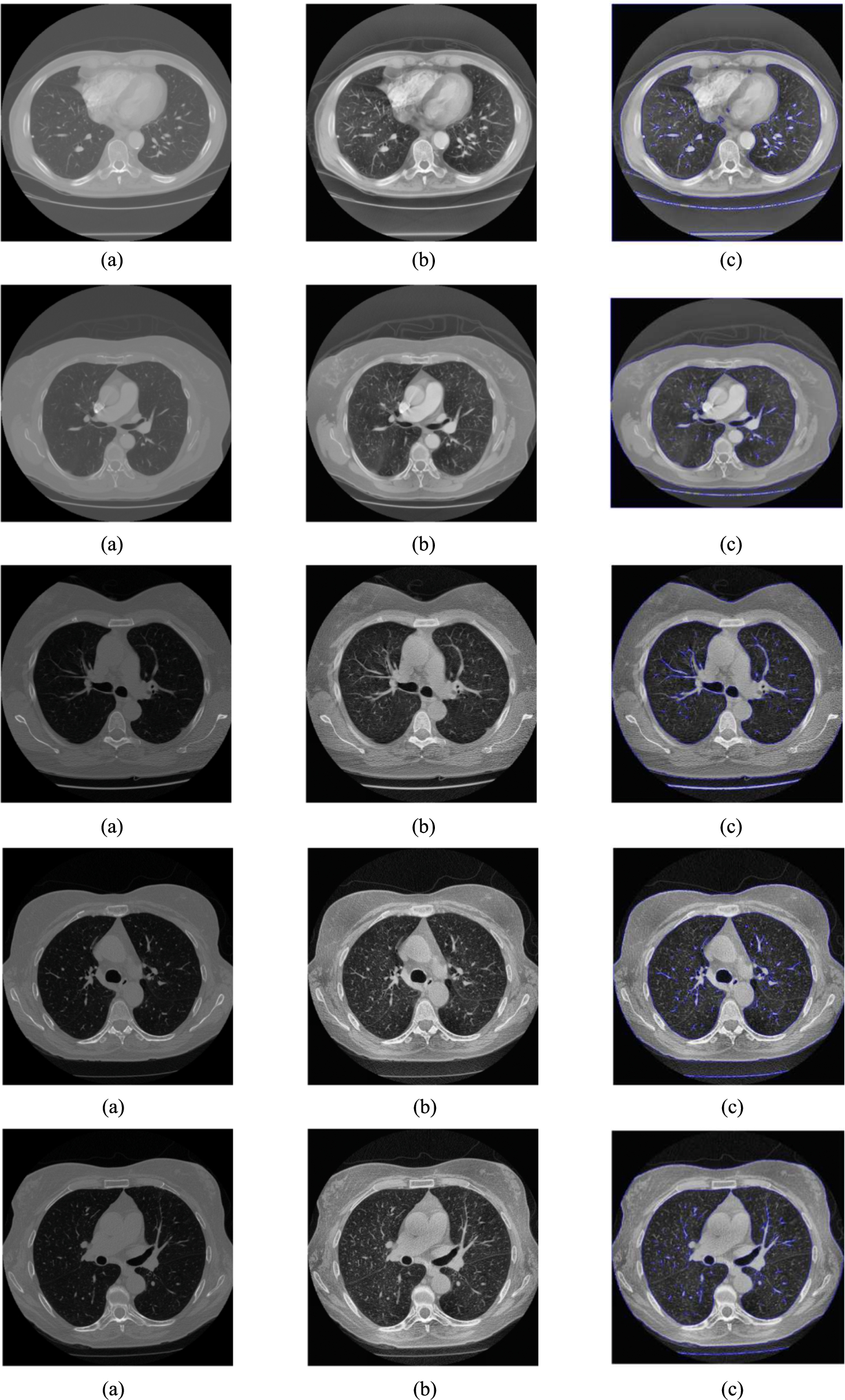
Sample images of dataset showing (a) input images (b) pre-processed images (c) level set segmentation images.

Fig. 4.

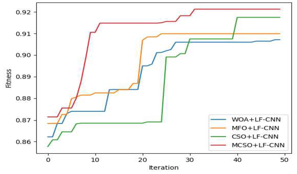
Convergence analysis of adopted MCSO+LF-CNN scheme over other conventional methods.

7.3. Overall performance analysis

Table 3 compares the adopted MCSO+LF-CNN model’s overall performance analysis to those of other conventional models for specific training percentages and accuracy measures. From the table, it can be shown that the suggested MCSO+LF-CNN model outperforms other current schemes including DBN, SVM, CNN, WOA+LF-CNN, MFO+LF-CNN, & CSO+LF-CNN for nearly all training percentages. Similar to existing standard systems like DBN, SVM, CNN, WOA+LF-CNN, MFO+LF-CNN, and CSO+LF-CNN, the suggested MCSO+LF-CNN method achieved 5.32%, 3.58%, 3.04%, 2.22%, 2.06%, and 1.41% greater accuracy values for train percentage 90. Additionally, Table 3 shows that the suggested MCSO+LF-CNN model outperforms other conventional models including DBN, SVM, CNN, WOA+LF-CNN, MFO+LF-CNN, and CSO+LF-CNN by achieving maximum accuracies ( $8.77 \times 10^{+ 01}$ ) for just a training percentage of 70. To improve the original RPN and get over the typical CNN’s object detection limitations, the proposed LF-CNN is used in this study. The position and orientation of the object are not encoded by the conventional CNN. As opposed to the resnet, the suggested model uses 3D convolution layers instead of 2D ones, which is expected to make it more effective. The MCSO solves the drawbacks of poor tracking accuracy, sluggish tracking speed, and precocious convergence and is suggested for effectively setting the weight in LF-CNN. The results show that the performance of the chosen MCSO+LF-CNN approach is superior than that of the conventional models.

Table 3
Overall effectiveness of implemented and current programmes for various training percentages

Metrics Training percentage

50% 60% 70% 80% 90%

DBN [52] $7.36 \times 10^{+ 01}$ $7.81 \times 10^{+ 01}$ $8.39 \times 10^{+ 01}$ $8.40 \times 10^{+ 01}$ $8.72 \times 10^{+ 01}$

SVM [8] $7.49 \times 10^{+ 01}$ $7.89 \times 10^{+ 01}$ $8.39 \times 10^{+ 01}$ $8.62 \times 10^{+ 01}$ $8.88 \times 10^{+ 01}$

CNN [20] $7.56 \times 10^{+ 01}$ $8.06 \times 10^{+ 01}$ $8.43 \times 10^{+ 01}$ $8.68 \times 10^{+ 01}$ $8.93 \times 10^{+ 01}$

WOA+LF-CNN [26] $7.87 \times 10^{+ 01}$ $8.28 \times 10^{+ 01}$ $8.63 \times 10^{+ 01}$ $8.76 \times 10^{+ 01}$ $9.00 \times 10^{+ 01}$

MFO+LF-CNN [25] $7.95 \times 10^{+ 01}$ $8.33 \times 10^{+ 01}$ $8.66 \times 10^{+ 01}$ $8.78 \times 10^{+ 01}$ $9.02 \times 10^{+ 01}$

CSO+LF-CNN [12] $8.02 \times 10^{+ 01}$ $8.33 \times 10^{+ 01}$ $8.66 \times 10^{+ 01}$ $8.84 \times 10^{+ 01}$ $9.08 \times 10^{+ 01}$

MCSO+LF-CNN $8.43 \times 10^{+ 01}$ $8.72 \times 10^{+ 01}$ $8.77 \times 10^{+ 01}$ $8.98 \times 10^{+ 01}$ $9.21 \times 10^{+ 01}$

Metrics	Training percentage
DBN [52]	$7.36 \times 10^{+ 01}$	$7.81 \times 10^{+ 01}$	$8.39 \times 10^{+ 01}$	$8.40 \times 10^{+ 01}$	$8.72 \times 10^{+ 01}$
SVM [8]	$7.49 \times 10^{+ 01}$	$7.89 \times 10^{+ 01}$	$8.39 \times 10^{+ 01}$	$8.62 \times 10^{+ 01}$	$8.88 \times 10^{+ 01}$
CNN [20]	$7.56 \times 10^{+ 01}$	$8.06 \times 10^{+ 01}$	$8.43 \times 10^{+ 01}$	$8.68 \times 10^{+ 01}$	$8.93 \times 10^{+ 01}$
WOA+LF-CNN [26]	$7.87 \times 10^{+ 01}$	$8.28 \times 10^{+ 01}$	$8.63 \times 10^{+ 01}$	$8.76 \times 10^{+ 01}$	$9.00 \times 10^{+ 01}$
MFO+LF-CNN [25]	$7.95 \times 10^{+ 01}$	$8.33 \times 10^{+ 01}$	$8.66 \times 10^{+ 01}$	$8.78 \times 10^{+ 01}$	$9.02 \times 10^{+ 01}$
CSO+LF-CNN [12]	$8.02 \times 10^{+ 01}$	$8.33 \times 10^{+ 01}$	$8.66 \times 10^{+ 01}$	$8.84 \times 10^{+ 01}$	$9.08 \times 10^{+ 01}$
MCSO+LF-CNN	$8.43 \times 10^{+ 01}$	$8.72 \times 10^{+ 01}$	$8.77 \times 10^{+ 01}$	$8.98 \times 10^{+ 01}$	$9.21 \times 10^{+ 01}$

7.4. Performance analysis

With regard to several positive, negative, and other metrics, the performance study of the MCSO+LF-CNN algorithm is compared to certain other current systems including DBN, SVM, CNN, WOA+LF-CNN, MFO+LF-CNN, and CSO+LF-CNN. Figures 5, 6, and 7 display the related results in terms of positive, negative, and other metrics. Visual examination of the results reveals that the suggested effort demonstrates the highest quality results. By changing the training % from 40, 50, 60, 70, 80, and 90, respectively, all these evaluations are conducted. It is clear from looking at the proposed work’s correctness that it performed better for every adjustment in the learning percentage. Moreover, the accuracy (in Fig. 5 (a)) of adopted work at 90th training percentage is 92.94, which was superior than old models like DBN = 87.89, SVM = 87.9007, CNN = 88.419, WOA+LF-CNN = 90.3768, MFO+LF-CNN = 90.864, and CSO+LF-CNN = 91.826. In addition, the MCSO+LF-CNN model attains higher sensitivity as 92.89 at 90th training percentage, which is 5.08%, 4.85%, 4.52%, 3.16%, 1.94%, and 1.50% superior to the old approaches include DBN, SVM, CNN, WOA+LF-CNN, MFO+LF-CNN, and CSO+LF-CNN, accordingly. And presented work was attained the highest precision having specificity at 97% and 97% at the 90th training percentage, respectively. At last, the presented design exhibited significantly improved lung cancer identification. A presented design effectiveness is due to two factors: the model’s training remains hopeful, and layer fusion allows the model to be effective in identifying lung cancer with minimum loss.

Fig. 5.

Performance analysis of the adopted MCSO+LF-CNN schemes over other traditional schemes for (a) accuracy (b) sensitivity (c) specificity (d) precision.

Figure 6 depicts the negative metrics of the adopted and traditional models, including FPR, FNR, FDR, and FOR. A number of training percentages increases while the negative measures decrease, and as a result, an outstanding performance was recorded by the presented system. In comparison to other systems like DBN = 44.9967, SVM = 44.34, CNN = 37.206, WOA+LF-CNN = 30.7171, MFO+LF-CNN = 30.7171, and CSO+LF-CNN = 29.65, the FOR of the suggested work at the 80th training percentage is 19.78, that are the lowest value. Furthermore, at the 90th training percentage, the FPR and FDR of the MCSO+LF-CNN technique outperformed those of other systems including DBN, SVM, CNN, WOA+LF-CNN, MFO+LF-CNN, and CSO+LF-CNN. At training percentage = 80, the MCSO+LF-CNN approach had achieved a minimal FNR value of 8, which is 4.57%, 2.42%, 1.49%, 1.49%, 1.21%, and 1.12% better than other standard design such as DBN, SVM, CNN, WOA+LF-CNN, MFO+LF-CNN, and CSO+LF-CNN. Since the presented design had attained a least error measures; it’s much more significant for lung cancer identification.

Fig. 6.

Performance analysis of the adopted MCSO+LF-CNN schemes over other traditional schemes for (a) FPR (b) FNR (c) FDR (d) FOR.

Figure 7 shows the study of additional measures for the adopted and current models, including NPV, Recall, MCC, FMS, and threat score. In addition at the 80th training percentage, the recall of the MCSO+LF-CNN model is 5.08%, 4.85%, 4.52%, 3.16%, 1.94%, and 1.50% better than existing schemes includes DBN, SVM, CNN, WOA+LF-CNN, MFO+LF-CNN, and CSO+LF-CNN, etc. Additionally, the suggested work’s FMS at the 90th training percentage is 93.96, which is superior to the models already in use like DBN = 89.667, SVM = 89.709, CNN = 89.838, WOA+LF-CNN = 91.60, MFO+LF-CNN = 91.938947, and CSO+LF-CNN = 92.714864. Likewise, the adopted MCSO+LF-CNN model attains a maximum NPV as 92.524% at the 90th training percentage. Additionally, MCC, threat score of the suggested design is higher. As a result, it is clear from the assessment that the suggested MCSO+LF-CNN system has the greatest result, and is hence said to be much more appropriate for lung cancer detection.

Fig. 7.

Performance analysis of the adopted MCSO+LF-CNN schemes over other traditional schemes for (a) NPV (b) FMS (c) MCC (d) recall (e) threat score.

7.5. Statistical analysis

Table 4 compares the statistical correctness of the proposed MCSO+LF-CNN technique to that of other industry-standard technologies. The suggested work is run numerous times, and the best results are compiled in Table 4 due to the stochastic nature of meta-heuristic algorithms. Its mean performance of a MCSO+LF-CNN is 91.57753086, which represents the best result. It performs better than other models like the DBN, SVM, CNN, WOA, MFO, and CSO+LF-CNN, which have mean performances of 89.114, 89.530, 90.103, and 83.215, respectively. In this study, the suggested LF-CNN is used to improve the original RPN in order to get over the classic CNN’s object detection-focused limitations. The location and the object’s orientation are not encoded by the conventional CNN. The proposed model is encouraged to be superior than the resnet as it replaces the 2D with 3D convolution layers. For optimally tuning the weight in LF-CNN proposes the MCSO overcomes the drawback of poor tracking accuracy, slow tracking speed, and precocity convergence. Thus the proposed method (LF-CNN+MCSO) provides better performance than the conventional method.

Consequently, the proposed model’s improvement has been successfully validated.

7.6. Discussion

Section 3 analyses the effectiveness of the proposed research’s ideal LF-CNN and compares the outcomes with those of other existing techniques like DBN, SVM, CNN, etc. The accuracy, precision, F-measure, and other error measures are analyzed. From the results, we attained presented design outperforms another methods because of layer-fused CNN architecture. As per the proposed LF-CNN are as follow: multi-resolution and the multiple layers are used such as multi-size, multi-shape and multi-angle for region proposal generation. In the proposed LF-CNN, the 3 same set of layers like “convolutional layer, relulayer, and pooling layer” are considered as 1 set of layer and it is fused with another similar set of layer. The fused sets of layers are combined with the fully connected layer. The Multiple layers and multiple resolutions of the fusion process accurately predict the cancer regions. In this study, the recommended LF-CNN is used to improve the original RPN in order to get over the classic CNN’s object detection-focused limitations. The location & the object’s orientation are not encoded by the conventional CNN. The proposed model is encouraged to be superior to the resnet as it replaces the 2D with 3D convolution layers. For optimally tuning the weight in LF-CNN proposes the MCSO overcomes the drawback of poor tracking accuracy, slow tracking speed, and precocity convergence. Thus the proposed method (LF-CNN+MCSO) provides better performance than the conventional method.

Table 4
Statistical analysis of Dataset2 with respect to accuracy

Measures DBN [52] SVM [8] CNN [20] WOA+LF-CNN [26] MFO+LF-CNN [25] CSO+LF-CNN [12] MCSO+LF-CNN

Mean 83.06 83.75 86.21 89.11 89.53 90.10 91.57

Median 82.41 83.43 86.79 89.00 89.43 89.87 91.50

Standard deviation 3.12 3.55 2.26 0.81 0.90 1.22 0.98

Worst 79.87 79.87 82.31 88.24 88.52 88.71 90.07

Best 87.89 87.90 88.41 90.37 90.86 91.82 92.94

Measures	DBN [52]	SVM [8]	CNN [20]	WOA+LF-CNN [26]	MFO+LF-CNN [25]	CSO+LF-CNN [12]	MCSO+LF-CNN
Mean	83.06	83.75	86.21	89.11	89.53	90.10	91.57
Median	82.41	83.43	86.79	89.00	89.43	89.87	91.50
Standard deviation	3.12	3.55	2.26	0.81	0.90	1.22	0.98
Worst	79.87	79.87	82.31	88.24	88.52	88.71	90.07
Best	87.89	87.90	88.41	90.37	90.86	91.82	92.94

8. Conclusion

The new deep learning-assisted lung cancer detection methodology presented in this paper contains 4 main phases: “(i) Pre-processing (ii) Segmentation (iii) Feature extraction and (iv) Classification”. In this study, the proposed LF-CNN is used to improve the original RPN to get over the limitations of the conventional CNN that is intended for object detection. Traditional CNNs do not encode the object’s position or orientation. As it substitutes 2D for 3D convolution layers, the suggested model is expected to outperform the resnet. The MCSO is a solution that the LF-CNN suggests to solve the drawbacks of poor tracking precision, sluggish tracking speed, and premature convergence while setting the weights optimum. Finally, the accepted scheme was calculated in comparison to the previous models using various measures, including recall, FNR, MCC, FDR, Threat score, FPR, precision, FOR, accuracy, specificity, NPV, FMS, & sensitivity, if appropriate. As seen in the graph, the adopted MCSO+LF-CNN model outperformed other current models including DBN, SVM, CNN, WOA+LF-CNN, MFO+LF-CNN, and CSO+LF-CNN in terms of accuracy by 12.69%, 11.15%, 10.32%, 6.64%, 5.69%, and 4.86%. As a result, the output was effectively categorized.

References

https://en.wikipedia.org/wiki/Central_moment#:~:text=In%20probability%20theory%20and%20statistics,random%20variable%20from%20the%20mean.

https://en.wikipedia.org/wiki/Entropy_(information_theory)#:~:text=Entropy%20measures%20the%20expected%20(i.e.,of%20a%20coin%20toss%20(%20).

https://en.wikipedia.org/wiki/Statistic.

Adir,

Tirman,

Abramovitch,

Botbol,

Lutaty,

Scheinmann,

Davidovits et al., Novel non-invasive early detection of lung cancer using liquid immunobiopsy metabolic activity profiles, Cancer Immunology, Immunotherapy 67(7) (2018), 1135–1146. doi:10.1007/s00262-018-2173-5.

Akter,

M.A.

Moni,

M.M.

Islam,

J.M.

Quinn and

A.H.M.

Kamal, Lung cancer detection using enhanced segmentation accuracy, Applied Intelligence 51(6) (2021), 3391–3404. doi:10.1007/s10489-020-02046-y.

Al Mohammad,

S.L.

Hillis and

P.C.

Brennan, Radiologist performance in the detection of lung cancer using CT, Clinical Radiology 74(1) (2018), 67–75.

V.H.

Arul,

V.G.

Sivakumar,

Marimuthu and

Chakraborty, An approach for speech enhancement using deep convolutional neural network, Multimedia Research 2(1) (2019), 37–44.

Avci, A new intelligent diagnosis system for the heart valve diseases by using genetic – SVM classifier, Expert Systems with Applications 36(7) (2009), 10618–10626. doi:10.1016/j.eswa.2009.02.053.

Bugter,

S.E.

van Brummelen and

D.J.

Robinson, Towards the optical detection of field cancerization in the buccal mucosa of patients with lung cancer, Translational Oncology 12(12) (2019), 1533–1538. doi:10.1016/j.tranon.2019.07.018.

10.

S.B.

Chandanapalli,

R.E.

Sreenivasa and

L.D.

Rajya, Convolutional neural network for water quality prediction in WSN, Journal of Networking and Communication Systems 2(3) (2019), 40–47.

11.

Chang,

Jung,

Ke,

Song and

Hwang, Automatic contrast-limited adaptive histogram equalization with dual gamma correction, IEEE Access 6 (2018), 11782–11792. doi:10.1109/ACCESS.2018.2797872.

12.

S.-C.

Chu,

Tsai and

J.-S.

Pan, Cat swarm optimization, in: International Conference on Artificial Intelligence, LNCS, Vol. 4099, 2006, pp. 854–858.

13.

Deotale,

Kolekar and

Kondelwar, Self-adaptive particle swarm optimization for optimal transmit antenna selection, Journal of Networking and Communication Systems 3(1) (2020), 1–10.

14.

Funai,

Honzawa,

Suzuki,

Momiki,

Asai,

Kasamatsu,

Kawase et al., Urinary fluorescent metabolite O-aminohippuric acid is a useful biomarker for lung cancer detection, Metabolomics 16(10) (2020), 1–8. doi:10.1007/s11306-020-01721-y.

15.

Gaddala and

Sangameswara Raju, Enhanced self adaptive bat algorithm for optimal location of unified power quality conditioner, Journal of Computational Mechanics, Power System and Control 2(3) (2019), 28–38. doi:10.46253/jcmps.v2i3.a4.

16.

George and

B.R.

Rajakumar, APOGA: An adaptive population pool size based genetic algorithm, in: AASRI Procedia – 2013 AASRI Conference on Intelligent Systems and Control (ISC 2013), Vol. 4, 2013, pp. 288–296.

17.

Ghimire,

Mundher Yaseen,

A.A.

Farooque,

R.C.

Deo,

Zhang and

Tao, Streamflow prediction using an integrated methodology based on convolutional neural network and long short-term memory networks, Scientific Reports 11(1) (2021), 1–26.

18.

Hao,

Pan,

Huang,

Wang and

Zhao, Sensitive detection of lung cancer biomarkers using an aptameric graphene-based nanosensor with enhanced stability, Biomedical Microdevices 21(3) (2019), 1–9. doi:10.1007/s10544-019-0409-6.

19.

Khatoon,

Fouad,

H.-K.

Seo,

O.Y.

Alothman,

Z.A.

Ansari and

S.G.

Ansari, Ethyl acetate chemical sensor as lung cancer biomarker detection based on doped nano-SnO₂ synthesized by sol-gel process, IEEE Sensors Journal 20(21) (2020), 12504–12511.

20.

LeCun,

Kavukvuoglu and

Farabet, Convolutional networks and applications in vision, in: International Symposium on Circuits and Systems, 2010, pp. 253–256.

21.

Liu,

Yao and

Wu, Deep reinforcement learning with its application for lung cancer detection in medical Internet of Things, Future Generation Computer Systems 97 (2019), 1–9. doi:10.1016/j.future.2019.02.068.

22.

Lu,

Y.A.

Nanehkaran and

Karimi Fard, A method for optimal detection of lung cancer based on deep learning optimized by marine predators algorithm, Computational Intelligence and Neuroscience (2021).

23.

Masood,

Sheng,

Yang,

Li,

Kim and

D.D.

Feng, Automated decision support system for lung cancer detection and classification via enhanced RFCN with multilayer fusion RPN, IEEE Transactions on Industrial Informatics 16(12) (2020), 7791–7801. doi:10.1109/TII.2020.2972918.

24.

Masood,

Yang,

Sheng,

Li,

Qin,

Lanfranchi,

Kim and

D.D.

Feng, Cloud-based automated clinical decision support system for detection and diagnosis of lung cancer in chest CT, IEEE journal of translational engineering in health and medicine 8 (2019), 1–13.

25.

Mirjalili, Moth-flame optimization algorithm: A novel nature-inspired heuristic paradigm, Knowledge-Based Systems 89 (2015), 228–249. doi:10.1016/j.knosys.2015.07.006.

26.

Mirjalili and

Lewis, The whale optimization algorithm, Advances in Engineering Software 95 (2016), 51–67. doi:10.1016/j.advengsoft.2016.01.008.

27.

Mohana,

S.A.

Sahaaya and

Mary, A comparitive framework for feature selection in privacy preserving data mining techniques using pso and k-anonumization, Iioab Journal 7(9) (2016), 804–811.

28.

Muthazhagan,

Ravi and

Rajinigirinath, An enhanced computer-assisted lung cancer detection method using content based image retrieval and data mining techniques, J Ambient Intell Human Comput (2020).

29.

Ojala,

Pietikainen and

Maenpaa, Multiresolution gray-scale and rotation invariant texture classification with local binary patterns, IEEE Transactions on Pattern Analysis and Machine Intelligence 24(7) (2002), 971–987. doi:10.1109/TPAMI.2002.1017623.

30.

Ozdemir,

R.L.

Russell and

A.A.

Berlin, A 3D probabilistic deep learning system for detection and diagnosis of lung cancer using low-dose CT scans, IEEE Transactions on Medical Imaging 39(5) (2020), 1419–1429. doi:10.1109/TMI.2019.2947595.

31.

Pang,

Zhang,

Ding,

Wang and

Xie, A deep model for lung cancer type identification by densely connected convolutional networks and adaptive boosting, IEEE Access 8 (2020), 4799–4805. doi:10.1109/ACCESS.2019.2962862.

32.

Pei,

Liu and

Dai, Discovering novel lung cancer associated antigens and the utilization of their autoantibodies in detection of lung cancer, Immunobiology 225(2) (2019), 151891.

33.

Pham,

Tao,

Zhang and

Yong, Constructing a knowledge-based heterogeneous information graph for medical health status classification, Health information science and systems 8(1) (2020), 1–14.

34.

Priyadharshini and

B.S.E.

Zoraida, Bat-inspired metaheuristic convolutional neural network algorithms for CAD-based lung cancer prediction, Journal of Applied Science and Engineering 24(1) (2021), 65–71.

35.

Priyanka and

Kumar, Feature extraction and selection of kidney ultrasound images using GLCM and PCA, Procedia Computer Science 167 (2020), 1722–1731. doi:10.1016/j.procs.2020.03.382.

36.

Radhakrishnan and

Kuttiannan, Comparative analysis of feature extraction methods for the classification of prostate cancer from trus medical images, IJCSI International Journal of Computer Science Issues 9(1) (2012).

37.

B.R.

Rajakumar, Impact of static and adaptive mutation techniques on genetic algorithm, International Journal of Hybrid Intelligent Systems 10(1) (2013), 11–22. doi:10.3233/HIS-120161.

38.

B.R.

Rajakumar, Static and adaptive mutation techniques for genetic algorithm: A systematic comparative analysis, International Journal of Computational Science and Engineering 8(2) (2013), 180–193. doi:10.1504/IJCSE.2013.053087.

39.

B.R.

Rajakumar and

George, A new adaptive mutation technique for genetic algorithm, in: Proceedings of IEEE International Conference on Computational Intelligence and Computing Research (ICCIC), Coimbatore, India, December 18–20, 2012, 2012, pp. 1–7.

40.

Sarkar, Optimization assisted convolutional neural network for facial emotion recognition, Multimedia Research 3(2) (2020).

41.

P.M.

Shakeel,

M.A.

Burhanuddin and

M.I.

Desa, Automatic lung cancer detection from CT image using improved deep neural network and ensemble classifier, Neural Comput & Applic (2020).

42.

P.M.

Shakeel,

M.A.

Burhanuddin and

Ishak Desa, Lung cancer detection from CT image using improved profuse clustering and deep learning instantaneously trained neural networks, Measurement 145 (2019), 702–712.

43.

P.M.

Shakeel,

Tolba,

Al-Makhadmeh and

M.M.

Jaber, Automatic detection of lung cancer from biomedical data set using discrete AdaBoost optimized ensemble learning generalized neural networks, Neural Comput & Applic 32 (2020), 777–790. doi:10.1007/s00521-018-03972-2.

44.

W.J.

Sori,

Feng,

A.W.

Godana,

Liu and

D.J.

Gelmecha, DFD-Net: Lung cancer detection from denoised CT scan image using deep learning, Frontiers of Computer Science 15(2) (2021), 1–13. doi:10.1007/s11704-020-9050-z.

45.

W.J.

Sori,

Feng and

Liu, Multi-path convolutional neural network for lung cancer detection, Multidim Syst Sign Process 30 (2019), 1749–1768. doi:10.1007/s11045-018-0626-9.

46.

T.C.

Srinivasa Rao,

S.S.

Tulasi Ram and

J.B.V.

Subrahmanyam, Enhanced deep convolutional neural network for fault signal recognition in the power distribution system, Journal of Computational Mechanics, Power System and Control 2(3) (2019), 39–46. doi:10.46253/jcmps.v2i3.a5.

47.

S.M.

Swamy,

B.R.

Rajakumar and

I.R.

Valarmathi, Design of hybrid wind and photovoltaic power system using opposition-based genetic algorithm with Cauchy mutation, in: IET Chennai Fourth International Conference on Sustainable Energy and Intelligent Systems (SEISCON 2013), Chennai, India, 2013.

48.

Tao

et al., Mining health knowledge graph for health risk prediction, World Wide Web 23(4) (2020), 2341–2362. doi:10.1007/s11280-020-00810-1.

49.

Toğaçar,

Ergen and

Cömert, Detection of lung cancer on chest CT images using minimum redundancy maximum relevance feature selection method with convolutional neural networks, Biocybernetics and Biomedical Engineering 40(1) (2019), 23–39. doi:10.1016/j.bbe.2019.11.004.

50.

Tripathi,

Tyagi and

Nath, A comparative analysis of segmentation techniques for lung cancer detection, Pattern Recognit. Image Anal. 29 (2019), 167–173. doi:10.1134/S105466181901019X.

51.

Wang,

Zhang,

Zhong and

Yu, Design of polarization imaging detection system for lung cancer cells based on microfluidic chip, Journal of Medical Systems 43(4) (2019), 1–8.

52.

H.Z.

Wang,

G.B.

Wang,

G.Q.

Li,

J.C.

Peng and

Y.T.

Liu, Deep belief network based deterministic and probabilistic wind speed forecasting approach, Applied Energy 182 (2016), 80–93. doi:10.1016/j.apenergy.2016.08.108.

53.

Yang,

Cheng and

Liu, An integrative microfluidic device for isolation and ultrasensitive detection of lung cancer-specific exosomes from patient urine, Biosensors and Bioelectronics 163 (2020), 112290. doi:10.1016/j.bios.2020.112290.

54.

Zhan,

Wang and

Li, An electronic nose-based assistive diagnostic prototype for lung cancer detection with conformal prediction, measurement 158 (2020), 107588.

55.

Zu,

Yu and

Luo, Integration of platelet features in blood and platelet rich plasma for detection of lung cancer, Clinica Chimica Acta 509 (2020), 43–51.

Modified convolutional neural network for lung cancer detection: Improved cat swarm-based optimal training

Abstract

Keywords

Nomenclature

1. Introduction

2. Literature review

2.1. Related works

3. Overview of the proposed work: An architectural description

4.1. CLAHE model

4.2. Modified levelset segmentation

5. Feature extraction process: Texture, statistical, and color features

5.1. Texture features

5.2. Statistical features

5.3. Color features

6. Lung cancer classification: CNN with modified cat swarm optimization-based training

6.1. Optimized LF-CNN model

Table 2 CNN hyper parameters S. No Parameters 1. Epoch = 20 2. Batch size = 256 3. Activation Layer 4. Fully Connected Layer 5. Softmax Layer 6. Classification Layer 7. Hidden neuron layer 1 = 32, layer 2 = 32, layer 3 = 64

7.1. Simulation procedure

7.2. Convergence analysis

7.6. Discussion

References

Table 2
CNN hyper parameters

S. No Parameters

1. Epoch = 20

2. Batch size = 256

3. Activation Layer

4. Fully Connected Layer

5. Softmax Layer

6. Classification Layer

7. Hidden neuron layer 1 = 32, layer 2 = 32, layer 3 = 64