Convolution-based scatter correction using kernels combining measurements and Monte Carlo simulations

Abstract

One of the well-recognized challenge of Cone-Beam Computed Tomography (CBCT) is scatter contamination within the projection images. Scatter degrades the image quality by decreasing the contrast, introducing cupping and shading artifacts and thus leading to inaccuracies in the reconstructed values. The higher scatter to primary ratio experienced in industrial applications leads to even more important artifacts. Various strategies have been investigated to manage the scatter signal in CBCT projection data. One of these strategies is to calculate the scatter intensity by deconvolution of primary intensity using Scatter Kernel Superposition (SKS). In this paper, we present an approach combining experimental measurements and Monte Carlo simulations to estimate the scatter kernels for industrial applications based on the continuously thickness-adapted kernels strategy with a four-Gaussian modeling of kernels. We compare this approach with an experimental technique based on a two-Gaussian modeling of the kernels. The results obtained prove the superiority of a four-Gaussian model to effectively take into account both the contribution of object and detector scattering as compared to a two-Gaussian approach. We also present the parameterisation of the scatter kernels with respect to object to detector distance. This approach facilitates the use of a single geometry for calculation of scatter kernels over the whole magnification range of the acquisition setup.

Keywords

CBCT Scatter correction CIVA industrial NDT

1 Introduction

Scatter artifact is a serious problem associated with Cone Beam Computed Tomography (CBCT) due to its higher illumination area. It causes various artifacts such as streaks and cupping effect on the reconstructed images. These effects become become prominent in industrial applications due to higher scatter to primary ratio (SPR). As a result, several techniques have been adopted in the literature to reduce the scatter artifacts. One of these techniques is the projection wise scatter correction with deconvolution process using scatter kernel superposition (SKS) method [1 –4]. Whether analytically fitted or from plain measurements, scatter kernels are generally assumed radially symmetric and stationary.

There are many deconvolution techniques based on calculation of kernels using Monte Carlo simulations [1 , 4–6]. The object scatter kernel modeling is usually proposed using the two-Gaussian model as in [4 , 8]. However, since the internal structure of the detector panel is mostly kept anonymous to the user, most of these methods do not take into account a realistic modeling of the flat panel detector leading to the calculation of only object scatter kernels. To tackle this issue, the use of experimentally calculated kernels [9 –11] makes it possible to correct the scatter contributions due to both the object and the detector, without having to rely on an accurate 3D modeling of the detector. Kernels are usually derived from measurements using the slanted-edge method to compute the edge spread function (ESF) response. In these techniques, the scattered radiation is approximated by pencil-beam kernels with purely experimental [9] or analytically-fitted [10, 11] models, and sometimes thickness-dependent [9]. Their results demonstrate that the contribution of scatter glare in the detector is important: the long-tails creating a modulation transfer function (MTF) drop in the low-frequency domain. Those analytical kernels involve a single exponential [10] or Lorentzian [11] model, the use of multiple terms in fitting the kernels being reported subject to instabilities for high-frequency components [11]. A single term in the analytical kernel model is however not able to discriminate the scatter contributions. Sun et al. [4] proposed to account for the detector scatter during the initialization with two Gaussian terms, but this preprocessing-step prior to the iterative SKS deconvolution might not be sufficient either to accurately model the detector kernel variability with respect to the object thickness, notably to take into account the hardening of the beam spectrum. The respective contribution of detector and object scatter in the kernels should be more clearly identified within the iterative deconvolution process, tuning the kernels according to the material thickness and the magnification when appropriate.

The overall scatter correction process thus, requires correction from the scatter contribution of both object and detector. Whereas object scatter can be accurately simulated using MC simulations, the detector compositions may not be accurately modeled in the simulations due to the undisclosed model of the detectors by manufacturers. Therefore, experimental measurements are needed to accurately calculate the scatter kernels of the detector and to calibrate the weighting factor of the kernels.

In this paper, we focus on industrial applications and propose to combine experimental measurements and Monte Carlo simulations to calculate the kernels of the two main scatter contributions: object and the detector. We begin by describing a four-Gaussian modeling of the scatter kernels calculated from joining experimental method and simulation. We then compare this approach with an experimental approach based on a two-Gaussian modeling of kernels. We further describe the method of parameterization of scatter kernels over the object to detector distance. The acquisition setup and the material used are described in the next section. Finally the results obtained with the four-Gaussian model and the two-Gaussian model are compared for the reconstructions performed using the classical Feldkamp, Davis, and Kress (FDK) algorithm [12] with software CIVA [13]. CIVA is a NDT simulation platform developed at CEA which can combine deterministic approach and MC simulations for CT simulations.

2 Method

2.1 Combining experiment and simulation: Four-Gaussian model

The measured intensity I is the sum of primary intensity P and the scatter intensity S such that $I (x, y) = P (x, y) + S (x, y)$ (1) where, x, y represent the current pixel positions on the 2D projection. The scatter signal can be modeled as the sum of the scatter contributions from the object and the detector. For each contribution, a resulting kernel which has the weight of the scatter to primary ratio is determined. The total scatter signal S using the continuously-thickness adapted kernels [6] can then be modeled as: $S (x, y) = P (x, y) \otimes K (x, y, T) = P (x, y) \otimes (K_{o} (x, y, T) + K_{d} (x, y, T))$ (2) where, ⊗ represents convolution and K is the thickness T dependent scattering kernel having its contribution from the object and detector scattering. Subscript d and o stand for the detector and the object respectively.

The scatter kernel can be rewritten as $K (x, y, T) = k (T) K^{*} (x, y, T)$ (3) where, the weight k (T) to be applied to the unit-integral scatter kernel K^* is the sum of the weights from the object scattering k_o (T) and the detector scattering k_d (T) such that $k (T) = \iint K (x, y, T) d x d y = k_{o} (T) + k_{d} (T)$ (4)

To determine the detector kernel K_d (x, y, T), two setups were used in this study as described in Fig. 1. In the setup described in Fig. 1 a), a zirconium sheet of thickness 0.1 mm was placed with a tilt of around 5° on the aluminum slabs of different thicknesses assuming spatial isotropy. This setup provides the point spread function (PSF) after considering both object and detector scatter. In the second setup described in Fig. 1b), the zirconium plate was placed directly on top of the detector. This setup provides the PSF after considering only the detector scatter. The ESF was first calculated for both the setups. In order to reduce the noise in the calculation of the ESF, one-hundred acquisitions were averaged out. A line spread function (LSF) can then be found from the derivative of the ESF.

Fig.1

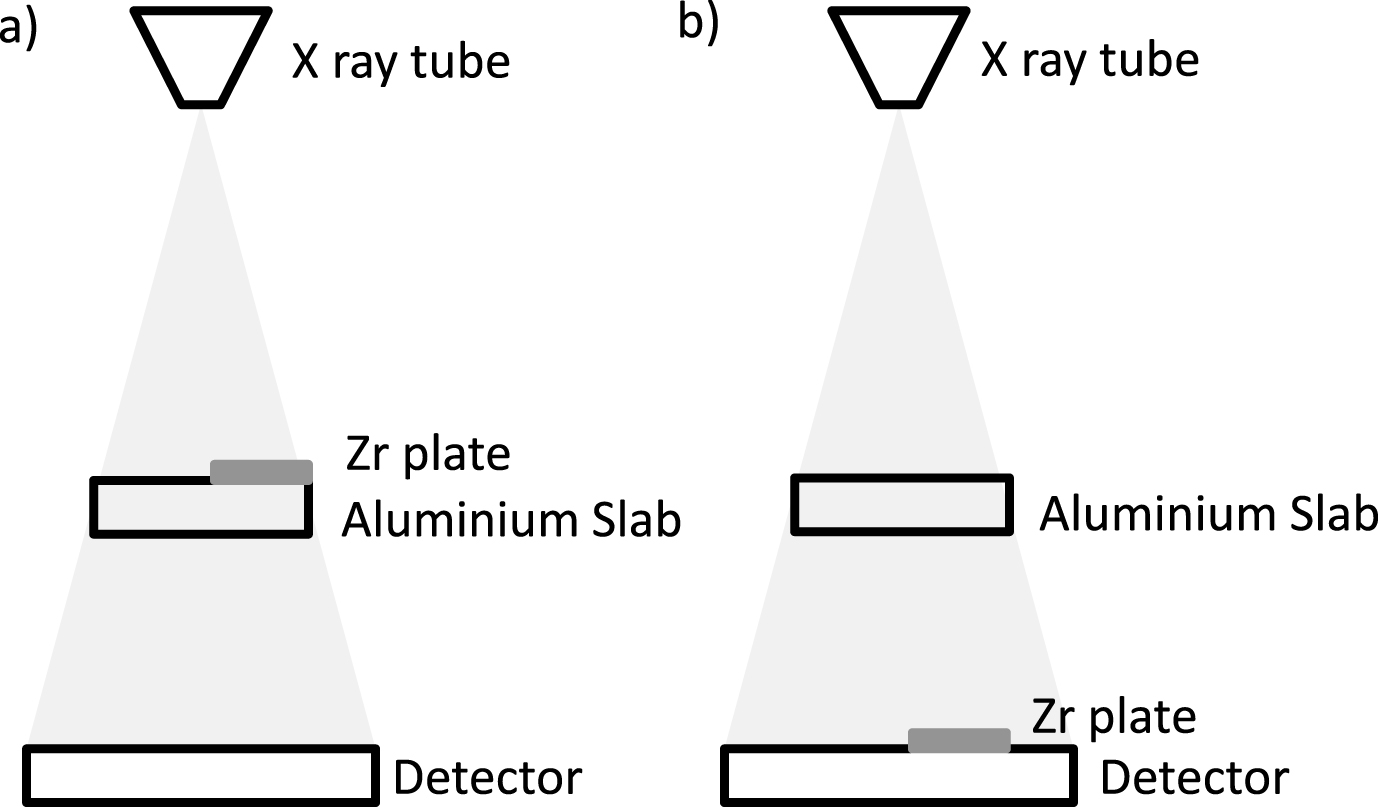
Schematic of the acquisition setup for the calculation of experimental kernels.

The object scatter kernels K_o (x, y, T) are determined by MC simulations as described in Bhatiaet al. [6].

For both the acquisition setups (Fig. 1) and for each material thickness, the obtained LSF was fit using a two-Gaussian model [6], given as $LSF (x, T) = \sum_{i = 1}^{2} A_{i} (T) exp (- \frac{x^{2}}{2 σ_{i}^{2} (T)})$ (5)

It should be noted that this two-Gaussian model is just to compute the weighting factor k (T) and not to model the scatter kernels. The relationship between PSF and LSF is given as $LSF (x, T) = \int_{- \infty}^{\infty} PSF (x, y, T) dy$ (6)

Therefore, the PSF of the LSF of form given in equation 6 is $PSF (x, y, T) = \sum_{i = 1}^{2} a_{i} (T) exp (- \frac{x^{2} + y^{2}}{2 σ_{i}^{2} (T)})$ (7) where $a_{i} (T) = \frac{A_{i} (T)}{\sqrt{2 π σ_{i}^{2} (T)}}$

From the PSF corresponding to the setup depicted in Fig. 1a) we have the following weight $W_{a} (T) = \iint {PSF}_{a} (x, y, T) d x d y \propto 1 + k_{o} (T) + k_{d} (T)$ (8)

Similarly for the setup in Fig. 1b) we have $W_{b} (T) = \iint {PSF}_{b} (x, y, T) d x d y \propto 1 + k_{d} (T)$ (9)

Combining the integral of the PSF measurements for the two setups gives $\frac{W_{b} (T)}{W_{a} (T) - W_{b} (T)} = \frac{1 + k_{d} (T)}{k_{o} (T)}$ (10)

The object weight factor k_o (T) is calculated using MC simulations (CIVA) and therefore, the weight factor of detector k_d (T) scatter can be calculated using $k_{d} (T) = \frac{W_{b} (T)}{W_{a} (T) - W_{b} (T)} k_{o} (T) - 1$ (11)

The final detector scatter kernels can then be calculated as $K_{d} (x, y, T) = (1 + k_{d} (T)) {PSF}_{b}^{*} (x, y, T) - δ [x, y]$ (12) where δ [x, y] is the Kronecker delta function and is null except for x = 0 and y = 0 where it is 1. Superscript ^* represents until normalized PSF.

Instead of using the Beer-Lambert law based on an effective linear attenuation coefficient μ, the thickness T at each pixel is directly computed from a look-up table f_BH –computed with CIVA for different slab thickness, that relates the true slab thickness with respect to the transmittance given by $T (x, y) = f_{BH} (\frac{P (x, y)}{O (x, y)})$ (13) where O is the unattenuated image. It is worthy of note that the beam-hardening is taken care of with this procedure. The acquisition parameters must be the same as the object under study. The choice of the calibration material is not critical: even if the sample is composed of several materials, as long as the energy spectrum is in the Compton dominant domain [6]. The directly transmitted primary fluency P was calculated for each thickness of the simulated slab. The thickness in terms of the transmittance P (x, y)/O (x, y) is then calculated as described in section 4.1.

The final scatter kernels were then fitted with a four-Gaussian model as follows $K (x, y, T) = \sum_{i = 1}^{2} w_{d, i} (T) exp (- \frac{x^{2} + y^{2}}{2 σ_{d, i}^{2} (T)}) + \sum_{i = 1}^{2} w_{o, i} (T) exp (- \frac{x^{2} + y^{2}}{2 σ_{o, i}^{2} (T)})$ (14) where, $k_{d} (T) = 2 π (w_{d, 1} (T) σ_{d, 1}^{2} (T) + w_{d, 2} (T) σ_{d, 2}^{2} (T))$ (15) and $k_{o} (T) = 2 π (w_{o, 1} (T) σ_{o, 1}^{2} (T) + w_{o, 2} (T) σ_{o, 2}^{2} (T))$ (16)

For generating the continuous map [6] of kernels, the amplitude parameters, w_d and w_o and the shape parameters σ_d and σ_o were also fit with respect to the thickness of the object.

2.2 Parameterisation of the kernels in terms of the distance

Acquisitions to calculate the scatter kernels can be tricky and time consuming for different sets of geometrical conditions. We propose a practical solution to correct the scatter over the whole magnification range by analytical parameterisation of object scatter kernels over the distance between the center of the object (where the rotational axis lies at the center of the object) and the detector. We call this distance d_OD for future reference. For this, we propose to acquire the detector kernels using the setup in Fig. 1b) assuming that the detector kernels do not vary over the magnification. We then analytically fit the parameters of the simulated object kernels over d_OD. Objects in the case of kernels calculations, refer to the slabs which are centered on the rotation axis.

The amplitude parameters of the object scatter kernels are expected to decrease over the increase in d_OD whereas kernel widths, given by sigma, of the two Gaussians are expected to increase over d_OD: the object scattering kernels progressively become flatter.

We describe these parameters as a power function of the distance d_OD with respect to a reference distance d₀ as: $p (T, d_{OD}) = p (T, d_{0}) {(\frac{d_{OD}}{d_{0}})}^{α}$ (17) where p∈ { w_o,1, w_o,2, σ_o,1, σ_o,2 } is any of the thickness T dependent parameters of the object scatter kernels. We expect the parameter α to be negative in case of amplitude parameters and positive in the case of standard deviation parameters. Note that if the differential cross section of the Compton scattering was isotropic in the considered energy range and if the sample was a small volume of scattering materiel in vacuum, the standard deviations would vary linearly with object-to-detector distance and the weights inversely proportional to it. Therefore in order to account for deviation from this ideal case, we proposed this single-parameter power law in equation 13.

2.3 Pure experimental approach: two-Gaussian model

In order to form a pure experimental approach, we calculated the weight factor $\bar{k} (T)$ using the ratio of experimental transmittance and theoretical transmittance calculated by the Beer-Lambert law, giving $\bar{k} (T) = \frac{E_{trans} (T)}{T_{trans} (T)} - 1$ (18) where, E_trans (T) represents the experimental transmittance obtained from experimental kernels and T_trans (T) is the theoretical primary transmittance calculated according to the Beer-Lambert law.

The experimental transmittance was calculated corresponding to the setup shown in Fig. 1a) such that $E_{trans} (T) \propto \frac{W_{a} (T)}{W_{a} (0)} \propto \frac{1 + k_{o} (T) + k_{d} (T)}{1 + k_{d} (0)}$ (19)

Therefore in reality, using equation 18, $\bar{k} (T)$ corresponds to $\bar{k} (T) = \frac{k_{o} (T) + k_{d} (T) - k_{d} (0)}{1 + k_{d} (0)}$ (20)

Therefore, to compute an estimate of the kernel weight k (T) using a solely experimental approach, the kernels weight of the detector scatter without object k_d (0) must be assumed to be negligible.

The final kernels of the setup in Fig. 1a) were then fitted with a two-Gaussian model as $K (x, y, T) = w_{d, 1} (T) exp (- \frac{x^{2} + y^{2}}{2 σ_{d, 1}^{2} (T)}) + w_{o, 1} (T) exp (- \frac{x^{2} + y^{2}}{2 σ_{o, 1}^{2} (T)})$ (21) where, $\bar{k} (T) = 2 π (w_{d, 1} (T) σ_{d, 1}^{2} (T) + w_{o, 1} (T) σ_{o, 1}^{2} (T))$ (22)

The result obtained with this method was compared with the results obtained using the four-Gaussian model described in section 2.1.

3 Material

3.1 Acquisition set up for aluminum cylinder

The acquisition setup mainly consisted of an X-ray source, an object rotational table and a flat panel detector. The X-ray source unit with 150 kV voltage, 750 mA current and the focal size of around 120 microns was used. Filtration consisted of a 0.3 mm aluminium inside the tube and a 1.5 mm external aluminium filter. Figure 2 shows simulated spectrum with internal and external filters at 150 kV source voltage. Figure 3 shows the variation of the mass attenuation coefficient of aluminium over the energy. The data was taken from NIST tables [14]. The flat panel detector used had an array size of 1024 × 1024 with 0.2 mm of pixel size.

Fig.2

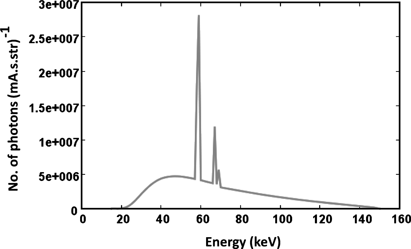
Simulated spectrum with internal and external filters at 150 kV source voltage with MCNP [15].

Fig.3

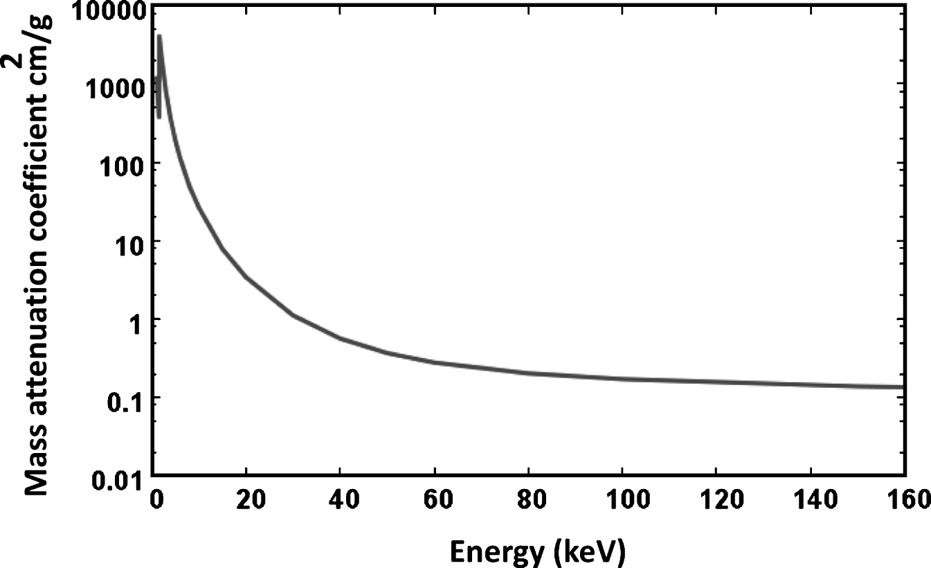
Variation of mass attenuation coefficient of aluminium over energy [14].

Acquisitions were performed on an aluminium cylinder as given in Fig. 4 with a diameter of 60 mm. The aluminium cylinder consisting of one central air insert (10 mm diameter) and three peripheral air inserts (3 mm diameters).

Fig.4

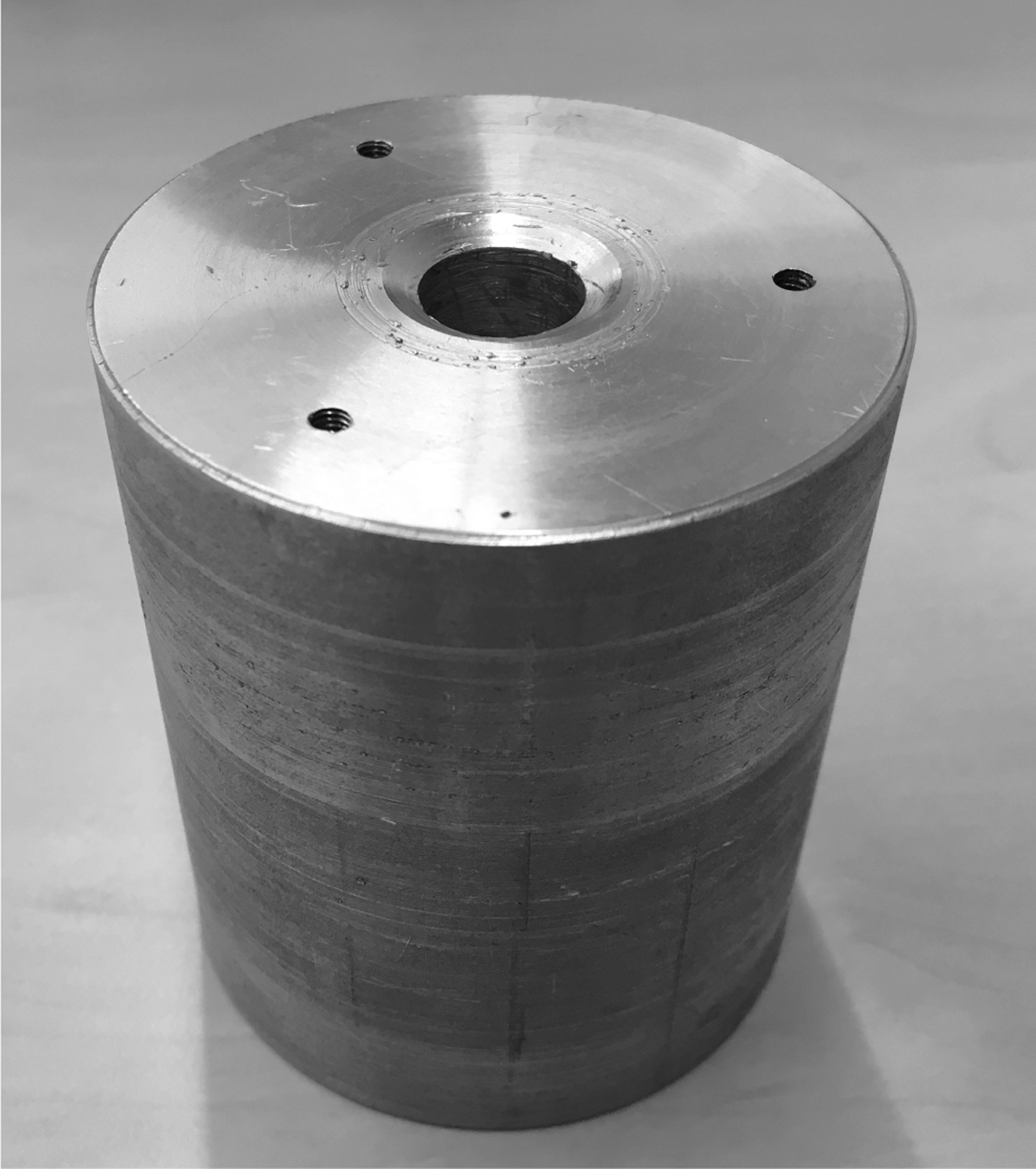
Picture of the aluminium cylinder with one central air insert (10 mm diameter) and three peripheral air inserts (3 mm diameters).

Two different magnification setups were used in order to validate the parameterisation of kernels in terms of different d_OD. In the first case, d_OD was 95 mm, whereas in the second case it was 295 mm. The source to detector distance was kept 600 mm in both cases.

4 Results

4.1 Analytical fitting of calculation of thickness: Beam-hardening correction

In order to calculate the thickness at each pixel, simulation was performed with slabs of different thicknesses. The directly transmitted primary fluency P was calculated for each thickness of the simulated slab. The thickness vs transmittance LUT f_BH given in equation 13 has been analytically calculated using least square fitting as shown in Fig. 5. The classical thickness determination based on the effective linear attenuation coefficient is also shown by the blue curve in Fig. 5. The beam-hardening, although not really strong, is taken care of with this procedure. Equation 23 gives the relationship of thickness T value in terms of transmittance P (x, y)/O (x, y). 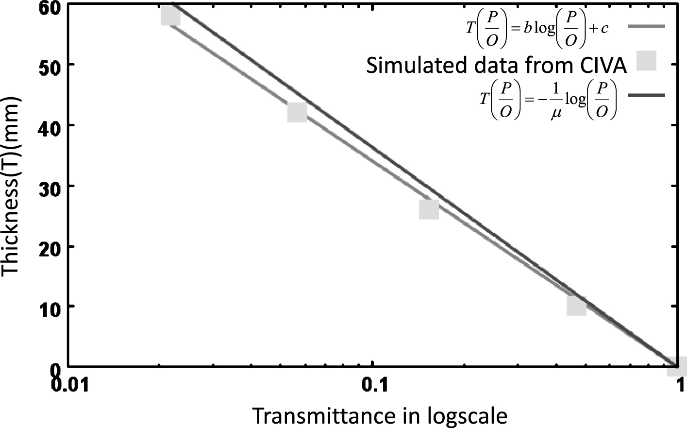$\begin{matrix} T (x, y) & = f_{BH} (\frac{P (x, y)}{O (x, y)}) \\ = b (\log (\frac{P (x, y)}{O (x, y)})) + c \end{matrix}$ (23) using b = -14.1, c = 1.14

Fig.5

Thickness (in mm) vs transmittance: MC simulations (green squares), analytical model (red curve) and monoenergetic curve (blue line).

4.2 Four-Gaussian model

Table 1 gives the calculated weighting factor k (T) and k_d (T) using the PSF areas W_a (T) and W_b (T) and the simulated weighting factor k_o (T) for object kernels of different thicknesses using equation 11.

Table 1
Table summarizing the calculated weighting factor k (T) and k_d (T) using PSF areas W_a (T) and W_b (T) and the simulated weighting factor k_o (T) for object kernels of different thicknesses

Thickness (mm) W_a (T) (pixel²) W_b (T) (pixel²) k_o (T) k_d (T) k (T)

10 1867 1760 0.12 0.99 1.12

26 621 555 0.32 1.68 2.00

42 587 493 0.70 3.27 3.02

58 955 807 1.10 4.99 6.10

Thickness (mm)	W_a (T) (pixel²)	W_b (T) (pixel²)	k_o (T)	k_d (T)	k (T)
10	1867	1760	0.12	0.99	1.12
26	621	555	0.32	1.68	2.00
42	587	493	0.70	3.27	3.02
58	955	807	1.10	4.99	6.10

The analytical description of the scatter kernels using the four-Gaussian model in comparison to the two-Gaussian model, can separate the low frequency contribution of scatter due to the object and the high frequency contribution of the detector. Moreover, we observed that the two-Gaussian model is not sufficient to fully take into account the contribution of the lower frequency scatter from the object. Table 2 shows a comparison of the fitting parameters for the two slab thicknesses (10 mm and 42 mm) with the two-Gaussian model and the four-Gaussian model for the combined (detector and object) scatter kernels, both simulated with CIVA. It also displays parameters object scatter kernels alone. We notice that the two-Gaussian model only provides the amplitude parameters w_(d,1) and w_(d,2) and neglects the contribution of the parameters w_(o,1) and w_(o,2), which actually correspond to the object scatter kernels. We also notice the underestimation of CIVA detector modeling as compared to the real experimental measurements.

Table 2

Simulated kernels with CIVA: Comparison of the fitting parameters for the two slab thicknesses (10 mm and 42 mm) with the two-Gaussian model and the four-Gaussian model for combined detector and object scatter kernels obtained with CIVA. Table also displays the parameters of the object scatter kernels alone. All the values of σs are in pixels and amplitude factors w are in pixel²

Thickness (mm)	Model	Detector				Object
		w_d (1)	w_d (2)	σ_d (1)	σ_d (2)	w_o (1)	w_o (2)	σ_d (2)	σ_d (2)
		×10^-3	×10^-1		×10^-1	×10^-4	×10^-4	×10¹	×10¹
	Two-Gaussian	0.085	4.5	2.1	4.7
10	Four-Gaussian	0.076	4.2	2.5	4.8	0.27	2.0	1.0	2.9
	Two-Gaussian					0.25	1.8	1.0	2.9
	Two-Gaussian	1.8	1.3	4.6	4.8
46	Four-Gaussian	1.7	1.2	4.6	4.9	1	2.6	1.9	4.8
	Two-Gaussian					1	2.7	2.1	5.0

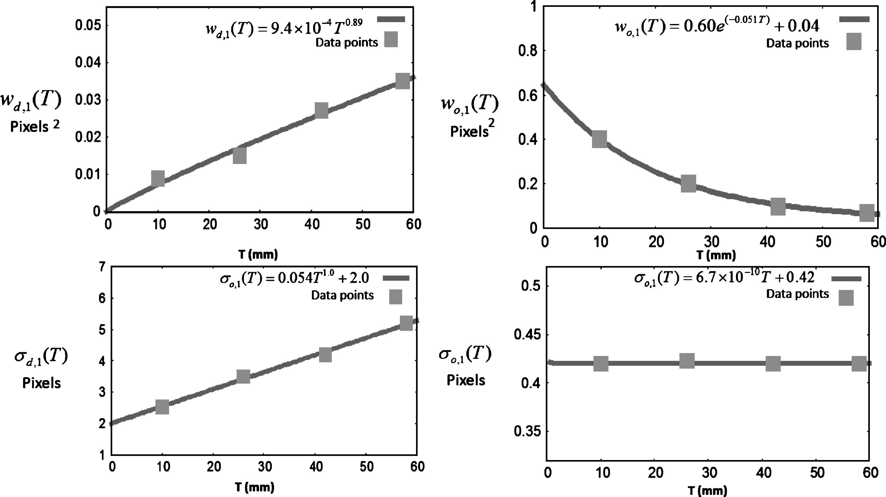
The noise level in the experimentally obtained LSF with the setup shown in Fig. 1 a) is high even after averaging over a hundred acquisitions, due to the noise coming from various sources such as quantum and electrical. Moreover, the output of the flat panel detector is limited by its optical transfer function. Therefore, we have designed the four-Gaussian model by a two Gaussian fitting of experimentally obtained detector kernels using the setup described in 1 b) and a two-Gaussian fitting of the object scatter kernels obtained from CIVA simulations. Figure 6 shows the experimentally calculated detector kernels and Fig. 7 shows the parameters of the fitting for the detector kernels. Figure 8 shows the simulated object kernels and Fig. 9 shows the parameters for the simulated object scatterkernels.

Fig.6

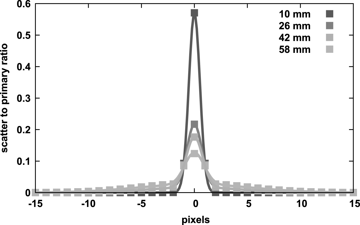
Plot profile of experimental detector kernels for different thicknesses for the setup in Fig. 1 b).

Fig.7

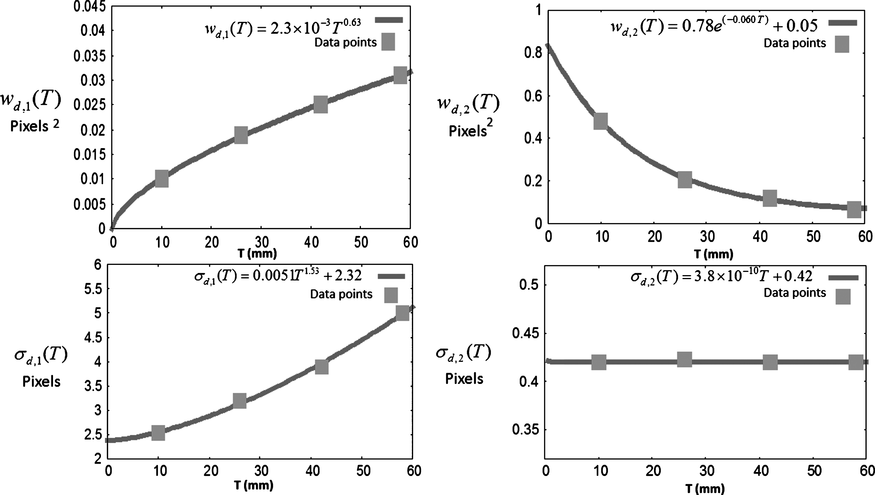
Fitting parameters of the experimental detector kernels using two Gaussian with respect to the thickness for the setup in Fig. 1 b).

Fig.8

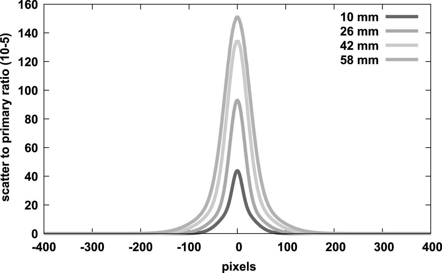
Plot profile of the simulated object kernels for different thicknesses.

Fig.9

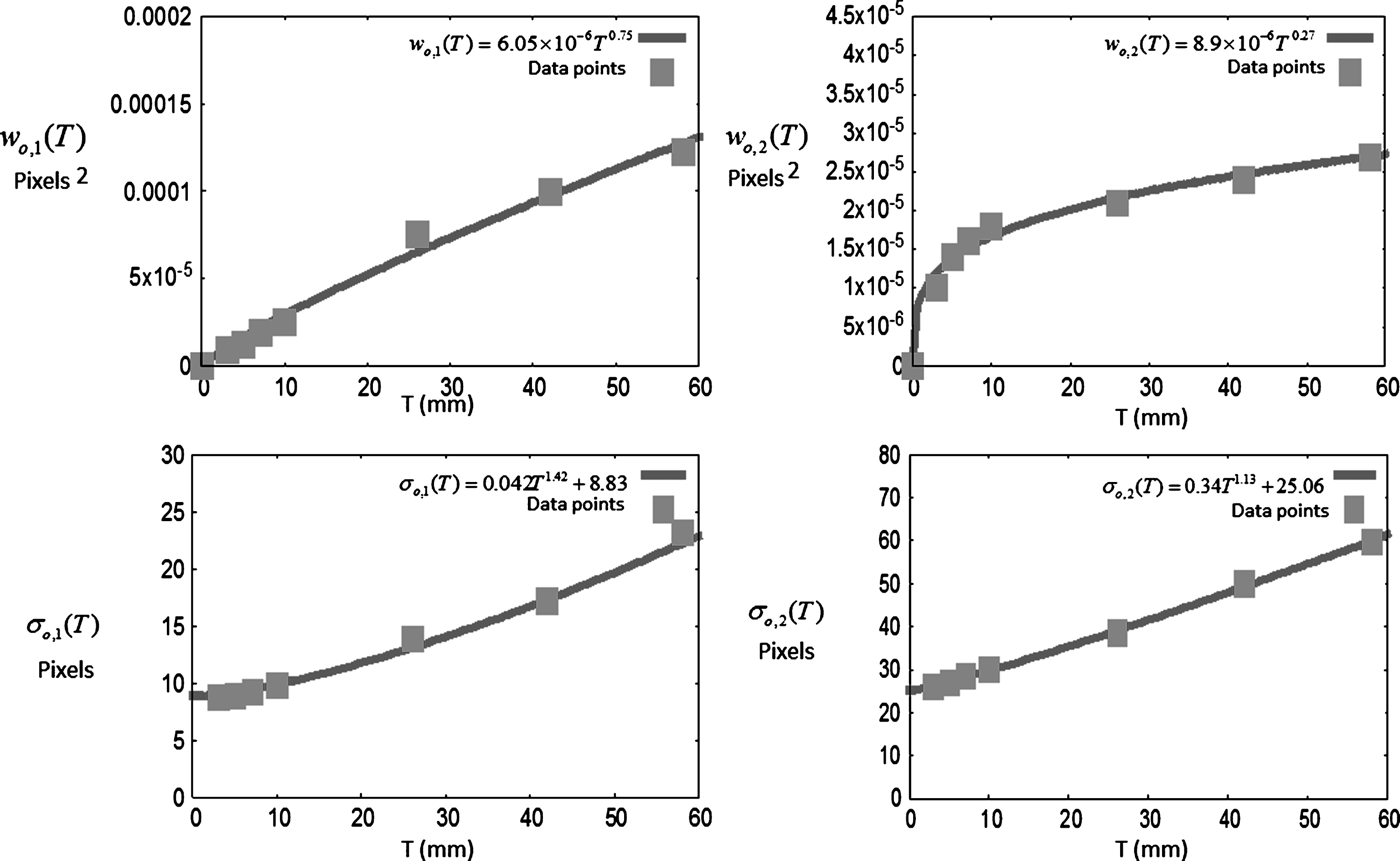
Fitting parameters of the simulated object scatter kernels using the two Gaussian terms with respect to the thickness.

4.3 Two-Gaussian model

As described in section 2.3, the weighting factor $\bar{k} (T)$ for each thickness of the slab is calculated using the experimental transmittance E_trans (T) and the theoretical transmittance T_trans (T) using equation 18. To form a continuous map for the application of continuous approach, $\bar{k} (T)$ was parametrized over the whole thickness range shown in Fig. 10. Figure 11 shows the plot profile of the experimental kernels derived for the setup in Fig. 1 a) for different thicknesses of aluminium slabs. The corresponding fitted parameters are plotted in Fig. 12.

Fig.10

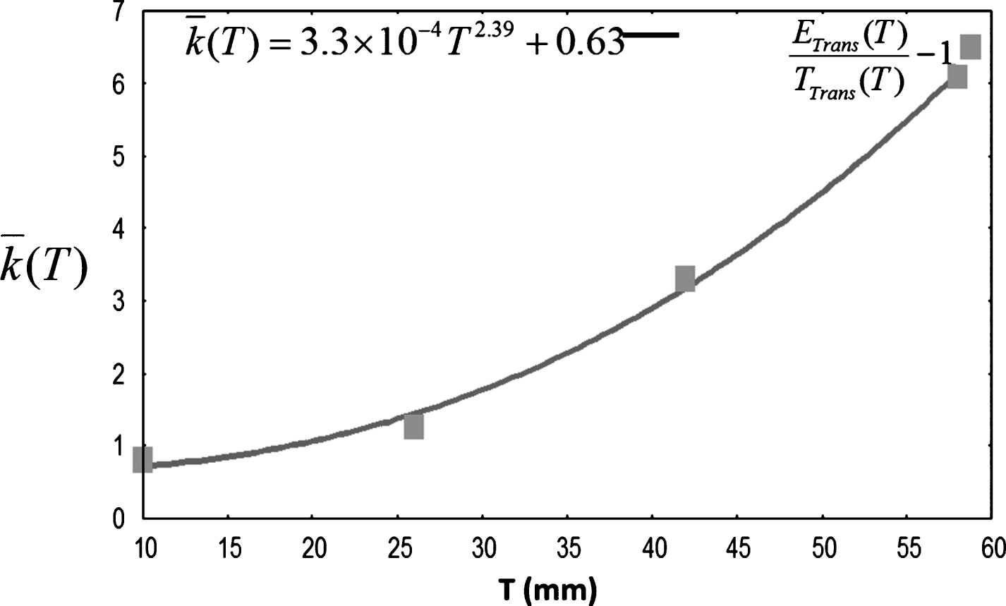
Continuous map of $\bar{k} (T)$ over the thickness calculated from the experimental transmittance and the theoretical transmittance

Fig.11

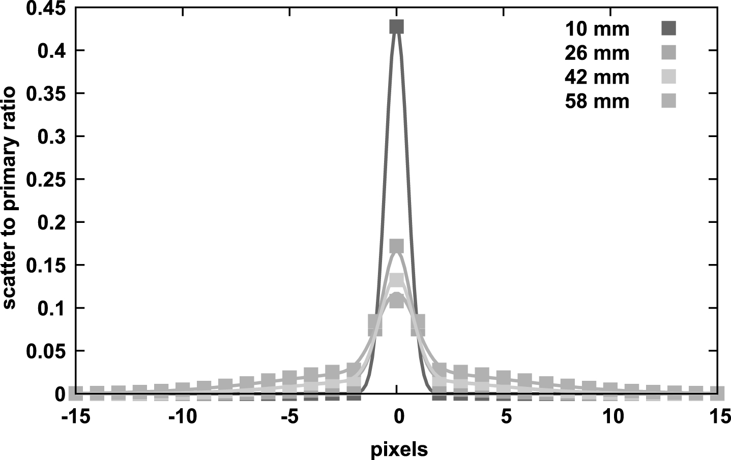
Plot profile of the experimental kernels for different thicknesses for the setup in figure 1a).

Fig.12

Fitting parameters of the experimental detector kernels using two Gaussian terms with respect to the thickness for the setup in Fig. 1a).

4.4 Parameterisation of the kernels with respect to distance

As described in section 2.2, we propose a parameterisation of the kernels in terms of d_OD in order to facilitate the use of a single geometry for the calculation of the scatter kernels over the magnification range of the acquisition setup. Figure 13 shows the object scatter kernels for a 10 mm aluminium slab for different d_OD. In Fig. 13, the kernels are normalized to the peak of kernel for d_OD = 95 mm.

Fig.13

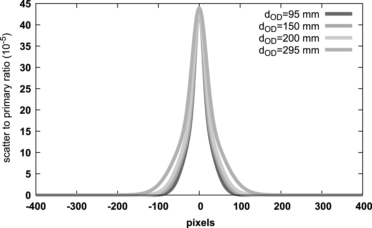
Normalized object scatter kernels over different object to detector distances for the T = 10 mm aluminium slab simulated with CIVA.

Figure 14 gives the fitting of the parameters of the object kernels for 10 mm slab over d_OD. The parameters were analytically fitted in as power functions in terms of d_OD as given in equation 17. We used four data sets of d_OD to perform this parameterisation. Figure 15 shows the relative absolute error in percentage between the simulated kernels and the parameterised kernels.

Fig.14

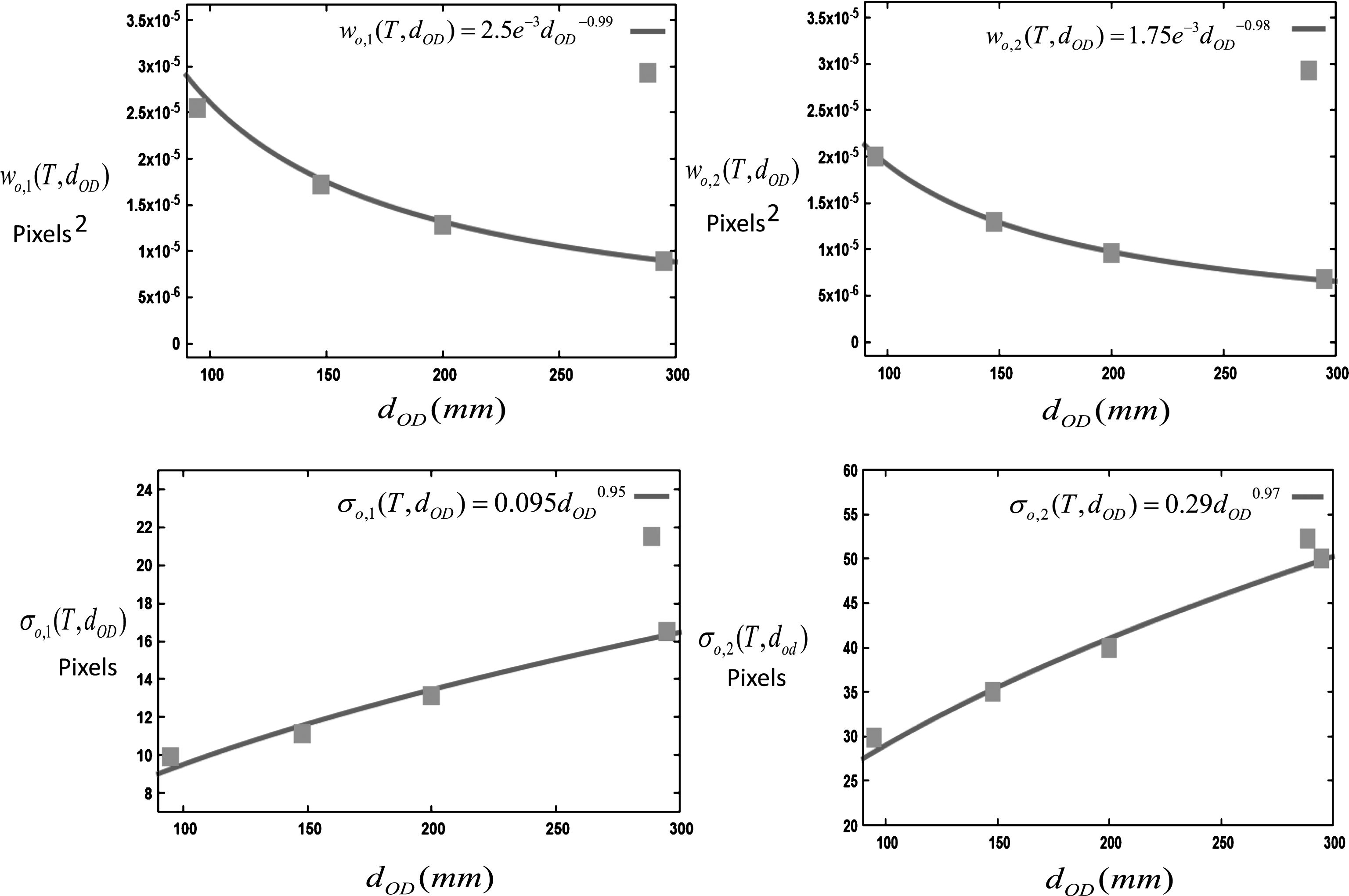
Fitting of parameters of the object scatter kernel for the T = 10 mm slab over the object-detector distance.

Fig.15

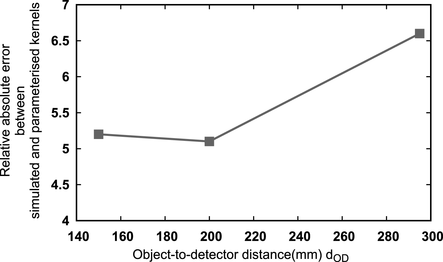
Relative absolute error between the simulated kernels and the parameterised kernels for the T = 10 mm slab.

4.5 Scatter correction on the aluminium cylinder

Figure 16a) shows the reconstruction obtained with the uncorrected projections. The red curve in the Fig. 17 shows the plot profile of this reconstruction with a clearly visible cupping effect. The green curve in Fig. 17 shows the result obtained with only beam hardening correction. Figure 16b) shows the reconstruction obtained after scatter and beam hardening correction using the two-Gaussian model and Fig. 16c) shows the reconstruction obtained after scatter and beam hardening correction using the four-Gaussian model.

The plot profiles of the reconstructions obtained after correction with the two-Gaussian and the four-Gaussian models are also shown in Fig. 17.

Fig.16

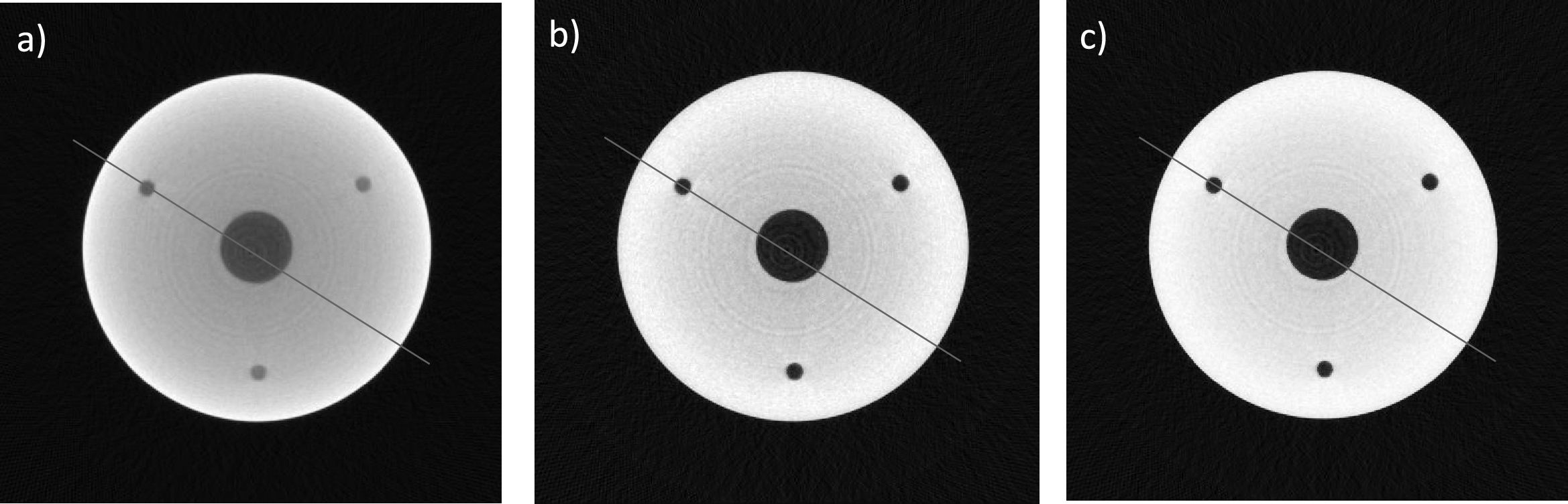
Reconstruction slice with a) uncorrected projections b) scatter and beam hardening corrected projections using the two-Gaussian model c) scatter and beam hardening corrected projections using the four-Gaussian model.

Fig.17

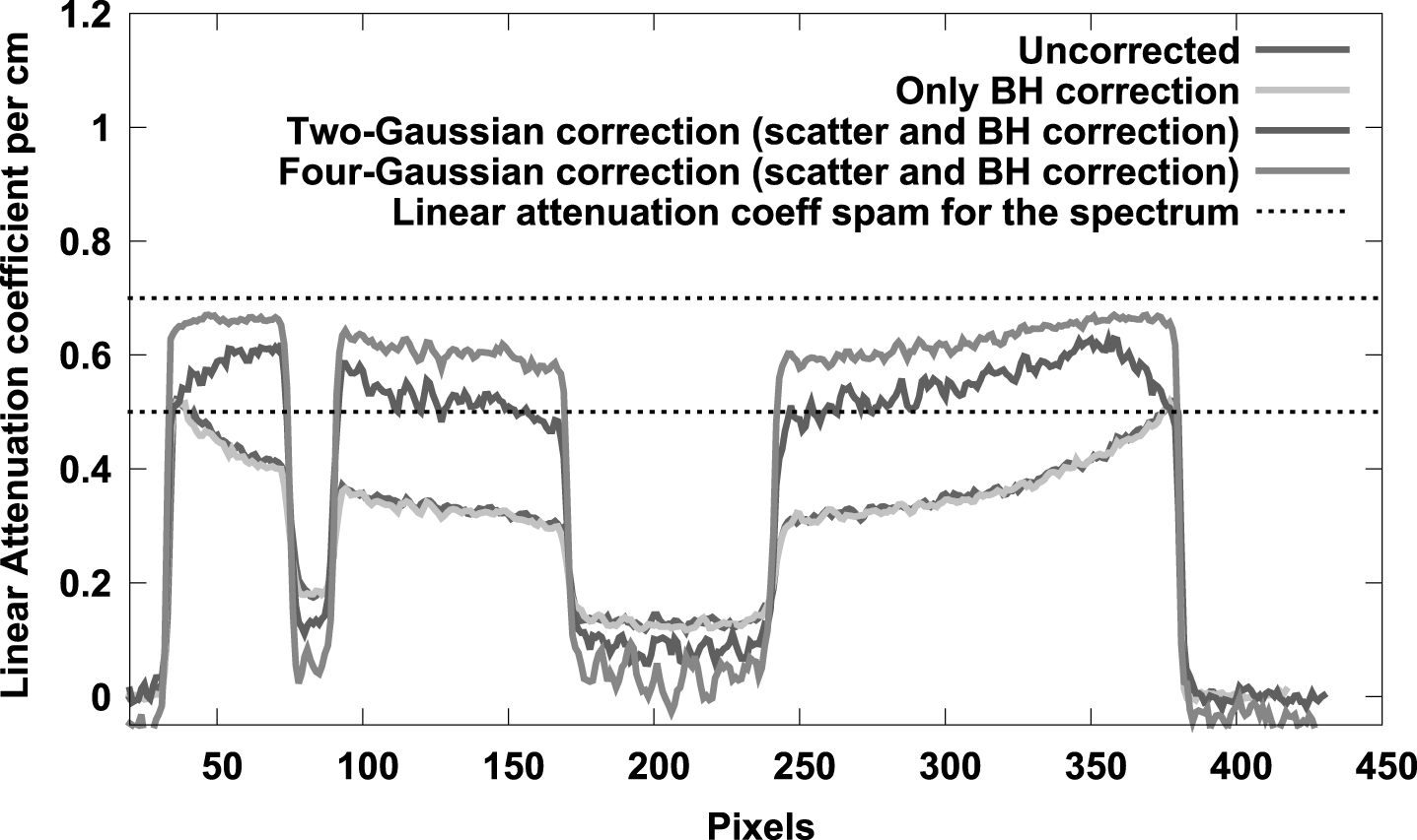
The plot profiles of the corrected and uncorrected reconstructions.

Table 3 displays the mean and the standard deviation of the reconstructed values for corrected and uncorrected data, in both air and aluminium region calculated using binary masks. Uncorrected value of 0.41 cm^-1 for the linear attenuation coefficient of aluminium is estimated. By using the two-Gaussian model, we obtain a value of 0.55 cm^-1 for the linear attenuation coefficient of aluminium. In the considered energy range (E ∈ [64 keV, 94 keV]), the value of the linear attenuation coefficient for aluminium lies between 0.5 cm^-1 at 64 keV and 0.7 cm^-1 at 94 keV. The relative absolute error in percentage is approximately 10% for the two-Gaussian model. Whereas, with the four-Gaussian model, we obtain a value of 0.62 cm^-1 for the aluminium. The relative absolute error is reduced to 3.4%.

Table 3

Mean and standard deviation values for aluminium and air region for uncorrected and corrected reconstruction slices

		mean (cm^-1) std. dev.
Uncorrected	air	0.132 ± 0.002
	aluminium	0.413 ± 0.007
Two-Gaussian correction	air	0.062 ± 0.006
	aluminium	0.552 ± 0.005
Four-Gaussian correction	air	0.060 ± 0.006
	aluminium	0.622 ± 0.009
Mean spectrum value	air	0.0001
	aluminium	0.614

Figure 18 shows the reconstruction obtained with simulated object kernels and the parameterised object kernels with respect to object-to-detector distance in the four-Gaussian model. Figure 19 shows the plot profile of these two reconstructions.

Fig.18

Reconstruction slice with a) simulated object kernels b) parameterised object kernels.

Fig.19

The plot profiles of the corrected reconstructions with simulated object kernels and parameterised object kernels.

5 Discussion

This paper presents a combination of experiments and simulations to calculate the scatter kernels for SKS method. The simulation of detector geometry is often tricky due to the lack of sufficient information of the detector geometry. Therefore, this paper presents an approach to calculate the detector PSF using experiments which takes into account this limitation of the MC simulation. Another important result presented in this paper is the thickness dependency of the PSF of the detector. The weighting factor of the detector kernels is not a single constant, as assumed in most of the previous studies, but rather it is a function of the thickness of the object present in front of the detector. This is due to the change in the spectrum by the presence of the object thickness. This is also evident from the variation of the parameter σ_d,1 related to the width of the Gaussian of the detector kernel, with the thickness of the object (Fig. 7).

We have shown the comparison of a four-Gaussian model with a classical two-Gaussian model of the scatter kernels. It shows that the four-Gaussian model clearly takes into account both the contribution of the object and the detector scattering whereas in the two-Gaussian model, the object contributions are not well taken into account. This results in a better reconstruction with the four-Gaussian model as compared to the two-Gaussian model.

Moreover, with the parameterisation of kernels with respect to the object-to-detector distance, only one set of kernels for a particular magnification are sufficient to recover the scatter corrected projections acquired at different setup geometries. We notice the effect of blurring in the kernels over the increase in object detector distance. This effect is also clear in the analytical fitting of the parameters of the kernels, where the amplitude factors of the kernels decrease over object detector distance whereas the width of the two Gaussians increases as a power function of the object-to-detector distance.

The effect of beam hardening is insignificant in this case and the improvement of the cupping effect is thus limited if only the correction of beam hardening is considered. This can be explained by the fact that, with the filtration used, the X-ray spectrum mainly lies within the energy of 25 keV to 120 keV. In this energy range, the linear attenuation coefficient of aluminium is almost steady subsequently leading to a minute beam hardening effect. However, we can also point out that the still remaining cupping artifact after correction can come from not so accurate modeling of the spectrum, which in that case, may produce the remaining beam hardening effect. We also observe that in the same energy range, if a material with high Z material, is used the variation in its linear attenuation coefficient is higher due to the higher probability of the interaction of photons in photoelectric domain. Moreover, in this energy range scatter correction of multi-material object is difficult because the probability of interaction is not dominantly Compton especially for high Z. Therefore, the likelihood of interaction is not just proportional to electron density and is dependent on the atomic number of the material.

The limitations of this technique are several. First during the calibration phase, a representative sampling of the equivalent attenuation ranges must be carried out, which means that the largest traversed material thickness has to lie in the attenuation range of the calibration (see equation 13). We also observed that a finer sampling towards low attenuation might sometimes be required (example in Fig. 9). The choice of the calibration material is however not crucial, even for multi-material sample, as long as the attenuation is mainly due to Compton scattering. This later requirement is the main limitation of the proposed method since it requires a specific energy range to be valid: not too low to avoid photo electric effect and not too high to avoid pair creation. This could be an issue for cargo screening application for example.

This proposed method can also perform for the CBCT half scan mode [16], where the black-hole scatter artifacts appears mainly due to presence of patient table top. Due to the presence of the table top as a source of scatter itself, a large amount of detected scatter for views where the tabletop is parallel, or nearly parallel, to the primary x-ray beam is detected. Only half of the lateral projections are affected due to the scatter contribution of the table top. As a result, the scatter from the table top is dependent on the angle of the projection. Therefore a weighted kernel with respect to the projection angle can be produced separately using simulations for the table top to handle the black hole artifact. Similar to the approach followed by Sun et al. [16], a hybrid kernel consisting of the sum of kernels due to object detector contribution plus a projection angle weighted kernel for table top scatter can be generated.

6 Conclusion

We presented a combination of experiments and simulations to calculate the scatter kernels for SKS method. Lack of information on the detector layout makes simulation unreliable, therefore in this paper, we presented an approach to calculate the detector PSF using experiments. Another important result presented in this paper is the thickness dependency of the PSF of the detector. The weighting factor of the detector kernels is not a single constant, as assumed in most of the previous studies, but rather it is a function of the thickness of the object present in front of the detector. This is due to the change in the spectrum by the presence of the object thickness. The parameters variations with respect to the object-detector distance are also presented, which facilitates working on different set-up geometries.

References

Hansen

V.N.

, Swindell

and Evans

P.M.

, Extraction of primary signal from EPIDs using only forward convolution, Med Phys 24(49) (1997), 1477–1484.

Spies

, Ebert

, Groh

B.A.

, Hesse

B.M.

and Bortfeld

, Correction of scatter in megavoltage cone-beam CT, Phys Med Biol 46 (2001), 821–833.

Maltz

J.S.

, Gangadharan

, Bose

, Hristov

D.H.

, Faddeg-ona

B.A.

, Paidi

and Hashemi

A.R.B.

, Algorithm for x-ray scatter, beam-hardening, and beam profile correction in diagnostic (kilovoltage) and treatment (megavoltage) cone beam CT, Transaction on Medical Imaging 27(12) (2008), 1791–1810.

Sun

, Star-Lack

J.M.

and Improved scatter correction using adaptive scatter kernel superposition, Phys Med Biol 55(22) (2010), 6675–6720.

Rinkel

, Gerfault

, Esteve

and Dinten

J.M.

, A new method for x-ray scatter correction: First assessment on a cone-beam ct experimental setup, Phys Med Biol 52 (2007), 4633–4652.

Bhatia

, Tisseur

, Buyens

and Létang

J.M.

, Scattering correction using continuously thickness-adapted kernels, NDT & E 78 (2016), 52–60.

Baer

, Kachelrieß

, Hybrid scatter correction for CT imaging, Phys Med Biol 57 (2012), 6849–6867.

Zhao

, Brunner

, Niu

, Schafer

, Royalty

, Chen

, Patientspecific scatter correction for at-panel detector-based cone-beam CT imaging, Phys Med Biol 60 (2015), 1339–1365.

, Mohan

, Zhu

, Scatter kernel estimation with an edge-spread function method for cone-beam computed tomography imaging, Med Phys 53 (2008), 6729–6748.

10.

Poludniowski

, Evans

P.M.

, Kavanagh

, Webb

, Removal and effects of scatter-glare in cone-beam ct with an amorphous-silicon at-panel detector, Med Phys 56 (2011), 1837–1851.

11.

Lazos

, Williamson

J.F.

, Impact of at panel-imager veiling glare on scatter-estimation accuracy and image quality of a commercial on-board cone-beam CT imaging system, Med Phys 39 (2012), 5639–5651.

12.

E. by Chris C Shaw, Cone Beam Computed Tomography.

13.

http://www-civa.cea.fr/.

14.

Berger

M.J.

, Hubbell

J.H.

, Seltzer

S.M.

, Chang

, Coursey

J.S.

, Sukumar

, Zucker

D.S.

, Olsen

, NIST XCOM: Photon cross sections database.

15.

Briesmeister

J.F.

, MCNP-A general Monte Carlo code for neutron and photon transport.

16.

Sun

, Nagy

, Virshup

, Partain

, Oelhafen

, Star-Lack

, Correction for patient table-induced scattered radiation in cone-beam computed tomography (CBCT)a, Med Phys 38.