Evaluation of noise limits to improve image processing in soft X-ray projection microscopy

Abstract

Soft X-ray microscopy has been developed for high resolution imaging of hydrated biological specimens due to the availability of water window region. In particular, a projection type microscopy has advantages in wide viewing area, easy zooming function and easy extensibility to computed tomography (CT). The blur of projection image due to the Fresnel diffraction of X-rays, which eventually reduces spatial resolution, could be corrected by an iteration procedure, i.e., repetition of Fresnel and inverse Fresnel transformations. However, it was found that the correction is not enough to be effective for all images, especially for images with low contrast. In order to improve the effectiveness of image correction by computer processing, we in this study evaluated the influence of background noise in the iteration procedure through a simulation study. In the study, images of model specimen with known morphology were used as a substitute for the chromosome images, one of the targets of our microscope. Under the condition that artificial noise was distributed on the images randomly, we introduced two different parameters to evaluate noise effects according to each situation where the iteration procedure was not successful, and proposed an upper limit of the noise within which the effective iteration procedure for the chromosome images was possible. The study indicated that applying the new simulation and noise evaluation method was useful for image processing where background noises cannot be ignored compared with specimen images.

Keywords

Soft X-ray projection microscopy iteration procedure noise evaluation

1 Introduction

Soft X-ray covers a wavelength region called water window where the X-ray absorption by water is significantly smaller than that by organic materials. This gives a possibility to observe the biological specimens in hydrated condition [1, 2]. Imaging with smaller radiation damage is also possible for the biological specimens compared with electron microscopy [3, 4].

Recent development in contact, scanning and imaging microscopes using soft X-rays enables us to obtain not only high spatial resolution imaging at a few tens of nanometer scale, but also three dimensional imaging of hydrated biological specimens with cryo-CT system [5 –10]. However, these types of microscopes except contact microscopy have relatively complex optical layouts. On the other hand, the projection type microscopy is composed of a simple optical layout without any precision mechanical stage required for the scanning type, and has advantages over other types of microscopy particularly for biological specimens [11, 12] such as its easy zooming function and easy extensibility to CT due to its wide viewing area.

One of the inherent problems in the projection microscopy is that the projection image is blurred by the diffraction of X-rays, resulting in the deterioration of spatial resolution. Yada and Takahashi tried to minimize the diffraction by setting a specimen very close to a point X-ray source around 100 nm diameter in a laboratory type projection microscopy using focused electron beam of scanning electron microscopy to produce a point X-ray source [13]. However such a system largely limited the possibility to CT in addition to the further improvement of spatial resolution. In our earlier studies, the blurred images have been corrected by an iteration procedure, which performs cycled calculations of Fresnel (FT) and inverse Fresnel (IFT) transformations [14 –17]. Further improvement such as contrast enhancement has been attempted prior to the iteration procedure to make the correction more effective and has partially succeeded in improving the correction level of those images [18, 19].

However, in some cases the correction was unsuccessful even in the situation where diffraction fringes were observable on projection images. In this case the diffraction fringes remained in the corrected images. In addition, when the contrast of projection images was very low, which was frequently experienced in the case of chromosomes, the diffraction fringes were hardly detected, resulting in the deformation of images after the iteration procedure. In this case the corrected images should be the same as the projection images. In other words, the morphology of the projection image should be unchanged in the iteration procedure. In this study, we addressed these problems from the viewpoint of the influence of background noises, because the contrast of diffraction fringes and the noises were comparable. We evaluated noise influence to the iteration effect by using simulation study. The simulation study was performed for the following two cases: One is for the chromosome images with relatively high contrast where the diffraction fringes were observable on the projection images. The other is for those with very low contrast where the diffraction fringes were not observable on the projection images.

(1) Evaluation of iteration effect for chromosome images with relatively high contrast:

In the images of chromosomes with relatively high contrast which were captured at a magnification of about 300 times, diffraction fringes remained on the images even after the iteration correction. To address this problem, we prepared a model projection image of known morphology containing diffraction fringes with high contrast similar to the chromosome images. Artificial noises were given to the image randomly and the upper limit of a ratio of the noise contrast to the contrast of the diffraction fringes, a newly introduced parameter (See “Materials and Methods”), was evaluated to achieve an effective correction by the iteration procedure.

(2) Evaluation of iteration effect for chromosome images with very low contrast:

In the images with very low contrast which were captured at magnification of 500–600 times, some or whole parts of the target were lost in corrected images after the iteration procedure. In this case, we prepared a model projection image whose contrast is adjusted to the same level of an experimental projection image of chromosome with a magnification of 504 times. Then the noise MSE (Mean Square Error; See “Materials and Methods”), another noise parameter, was introduced, and the relationship between noise MSE on the simulated projection image and contrasts of its corrected image were examined, and upper limit of noise MSE was determined where the morphology of the projection image was not changed after the correction.

2 Materials and methods

2.1 Projection experiment

We used a bending magnet beam line BL-11A as a monochromatic soft X-ray source at Photon Factory of KEK (High Energy Accelerator Research Organization) in Tsukuba, Japan. The BL-11A beam line provides soft X-rays in the energy range between 70 eV and 1900 eV with a grazing-incidence monochromator. In our study, monochromatic soft X-rays with the energy of 700 eV were selected by using a grating with groove density of 800 l/mm. In order to make a point source from soft X-ray beam, the optics of microscopy were constructed with a zone-plate and a pinhole which is located at a focal point of the zone-plate. Thus, the actual size of the source was determined as the size of the pinhole, although the theoretical value is calculated from the outermost zone width (80 nm).

Images were taken with a back-illuminated X-ray CCD camera of 12.3 mm square X-ray sensitive area with 24μm pixel-pitch (Hamamatsu Photonics C4880-30-26 W). A specimen was placed between the pinhole and the CCD camera and magnified images of the specimen were captured on the CCD screen as projection images. The magnification was adjusted by moving the specimen between the pinhole and the CCD screen. It was calculated as a ratio of distances from the pinhole to the CCD screen and to the specimen position based on its optical layout. The optical layout of the microscopy and the typical projection conditions are shown in Fig. 1 and Table 1, respectively. The focal distance of the zone plate was evaluated from diameter of its innermost zone (14.142μm) and wavelength of the soft X-ray (1.77 nm) [20]. The pinhole and other optical devices including specimens were installed in a vacuum chamber.

Fig.1

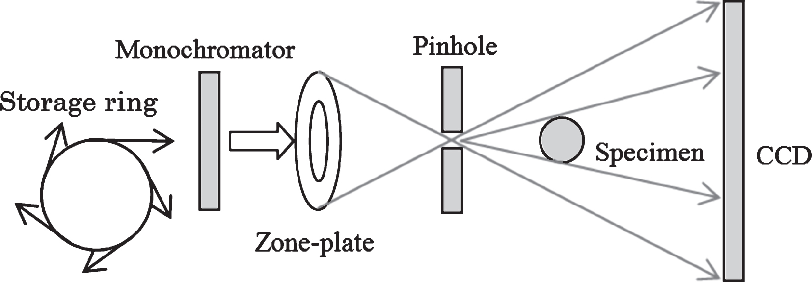
Optical layout of soft X-ray projection microscopy.

Table 1

Typical experimental conditions

–	Values
X-ray energy	700 eV
Focal distance of zone-plate	28.25 mm
Pinhole diameter	0.5 or 1μm
Distance between pinhole and CCD screen	329 mm
Distance between pinhole and specimen	0.5∼7 mm
Temporal coherence (Energy resolution)	0.89μm (1.4 eV)
Magnification	47∼658 times
Projection time	3 min

2.2 Specimen for imaging

Chromosome preparation was made from cultured human lymphocyte cell line (IM-9) on a silicon nitride window with 1 mm square in size and 100 nm in thickness supported by a center-hollowed silicon substrate with 5 mm square in size and 380μm in thickness according basically to the standard protocol for light microscopic observation with some minor modifications [21]. In brief, the cells in early logarithmic growth phase (2-3*10⁵ cells/ml) were arrested in mitotic phase by treating with 50μg/ml of colcemid at 37 °C for 5 hours and centrifuged at 1000 rpm for 5 min. The precipitated cells were resuspended in a hypotonic solution (75 mM of KCl or 0.5% of sodium citrate) at 37 °C, and kept for 20 min at the same temperature for swelling and then fixed with Carnoy fixative (a mixture of methanol/glacial acetic acid 3 : 1). A small volume (ca. 30–40μl) of the fixed cell suspension was dropped onto the silicon nitride window and air dried. In some cases, the window with chromosome specimen was washed with fresh fixative to remove cytoplasmic debris around the chromosomes before the specimen was dried up completely. The background of the window surface became rather clean with few losses of chromosomes by this wash.

2.3 Simulation and correction of projection images

In the simulation process, we prepared a model specimen of known morphology with the background illumination of X-rays which was obtained experimentally, because the critical factor which affects iteration calculation and results in lowering spatial resolution is supposed to be the spatial variation of X-ray illumination. Therefore, the correction of the illumination variation has been a main issue in our imaging experiments [18]. Thus, we also gave a gradation to the edge of the model specimen in order to mimic it to the periphery of the chromosome specimen.

For simulation of a projection image from the model specimen, X-ray propagation was performed from the specimen surface to the CCD screen by using FT calculation and distribution of the X-ray intensity on the CCD screen was calculated from its amplitude distribution. The noises on the projection image mainly due to X-ray scattering were simulated based on noise information of the experimental projection image and added them to the simulated projection image randomly. The correction effect by an iteration procedure which performs cycled calculations of FT and IFT was examined on a simulated projection image. Wavelength (energy) and propagation distance of the X-rays needed for the FT and IFT calculations were adjusted based on the experimental conditions. Other parameters needed for those calculations are amplitude and phase of X-rays. Details of the parameters are summarized in Fig. 2 with simulation and projection procedure of the projection image.

Fig.2

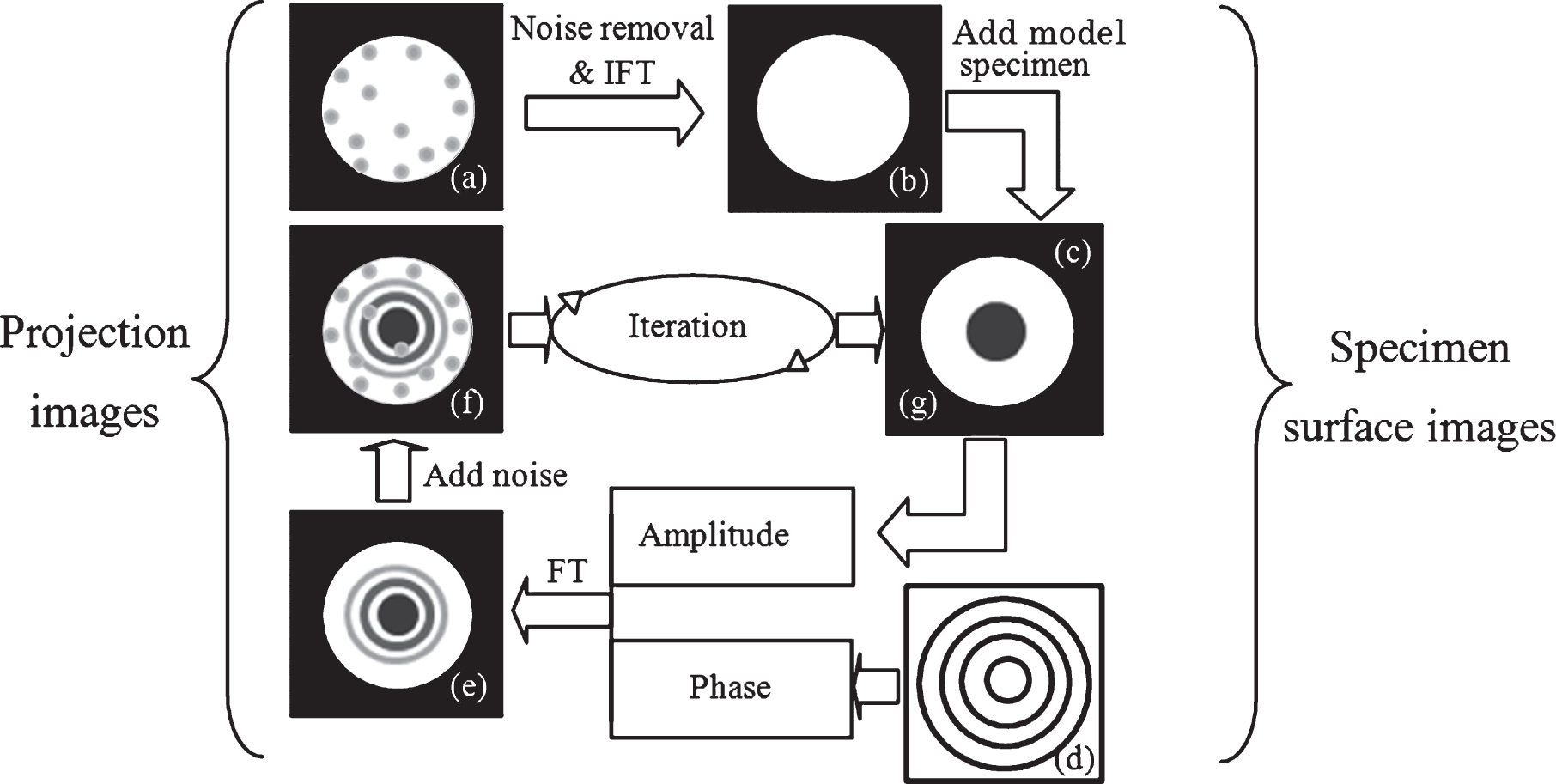
Simulation and correction procedure for projection image. (a) X-ray image of illumination by experiment, (b) X-ray image of illumination for simulation, (c) Specimen image, (d) Phase distribution of spherical wave, (e) Projection image without noise, (f) Projection image with noise, (g) Corrected image.

First, an X-ray image of illumination was captured experimentally (Fig. 2a), and the illumination image for simulation on the specimen surface (Fig. 2b) was obtained by removing background noise with a simple moving average process and by applying IFT on the image of Fig. 2a. Then the specimen image (Fig. 2c) was prepared by adding a model specimen with graduation edge on the image of Fig. 2b. Projection image of Fig. 2e was calculated by using FT. The calculation uses amplitude distribution from the specimen image (Fig. 2c) and phase distribution of spherical wave on the specimen surface (Fig. 2d), because X-ray spherical wave from a point source (pinhole) is used for our projection experiments.

Then, noise was added to the projection image (Fig. 2e) directly for the evaluation of the noise influences, leading to the projection image (Fig. 2f). The noise distribution was set up randomly, and the sizes and number of the noises were based on the noise information of experimental projection images for which the blur correction by the iteration procedure was not effective. Noise contrast, defined as a ratio of the difference between the highest and lowest value of intensity for the noise to the illumination intensity, was introduced as variables.

To correct the projection image (Fig. 2f), the iteration procedure was applied to X-ray intensity distribution on the surface of the specimen (Corrected image shown in Fig. 2g). In the iteration procedure, X-ray amplitude information on the projection image is obtained from the X-ray intensity distributions recorded on the CCD screen.

For the input of the iteration procedure, the projection image (Fig. 2f) was used because the same condition for the correction of the experimental projection images is necessary. As we do not have any information about X-ray phase distribution which is essential for the correction of the experimental projection image, the phase distribution of spherical waves was used as a first step. Then, the iteration procedure using cycled calculations of FT and IFT was introduced to deduce the approximate phase distribution on the experimental projection images. The repetition of the cycled calculations was stopped when the specimen boundary on the corrected image (Fig. 2g) is not changed even if further calculation is carried out.

The specimen boundary on the corrected image (Fig. 2g) was traced and checked to be equivalent or not to that of the projection image (Fig. 2f) for the judgment whether the correction was successful or insufficient in the case of very low contrast. On the other hand the diffraction fringes in the corrected image (Fig. 2g) were examined for the judgment whether the correction was successful or insufficient in the case with relatively high contrast where the diffraction fringes were observable on the projection image (Fig. 2f).

A contrast criterion of human eye’s threshold which could be distinguished target contrast of the difference of 2% against background intensity [22] was applied as a criterion of the specimen edge and the diffraction fringes.

The noise contrast divided by the contrast of diffraction fringe was adopted to evaluate the noise for the chromosome image with relatively high contrast, because some of the images with relatively high contrast were successfully corrected by adjusting the contrast of noise and diffraction fringes [18]. Therefore the ratio of the noise contrast to the contrast of diffraction fringes was considered as a good measure of noise in this case. The contrast of the diffraction fringes was defined similarly to the noise contrast as a ratio of the difference between the highest and lowest values of intensity for the diffraction fringes to the illumination intensity. A relationship between the contrast ratio in the projection image (Fig. 2f) and contrast of the diffraction fringes in the corrected image (Fig. 2g) was examined, because the problem in this case was that the diffraction fringes remained in the correctedimage.

On the other hand a relationship between contrast of target in the corrected image (Fig. 2g) and a noise MSE of the projection image (Fig. 2f) was studied for the chromosome image with very low contrast where the diffraction fringes were hardly detected and the contrast of target (specimen morphology) was lost by the iteration procedure. The noise MSE was adopted to evaluate the noise by taking all parameters of the noise (noise number, size and contrast) into account, because the images were not correctable even if the contrast enhancement was performed prior to the iteration procedure while some images with relatively high contrast were corrected effectively. The noise MSE was defined using equation (1) as a value of square grayscale per pixel [23]. $Noise MSE = \frac{1}{N} \sum_{n_{1}}^{N} {(G}_{n} {- G}_{n}^{0})^{2}$ (1)

Where, G_n and $G_{n}^{0}$ are grayscale value of n in a pixel of the projection image with noise (Fig. 2f) and that without noise (Fig. 2e), respectively. N (= 512*512) is total number of the image pixels.

To evaluate the contrast of target, we chose “equation (2)” based on the “Weber diffraction definition of contrast [24]”. $Contrast of target = \frac{| G_{1} - G_{2} |}{G_{\max}}$ (2)

where, G₁ is an average value of the grayscale distribution around the target in an area between the large square and the small square (Fig. 3). G₂ is an average value of the grayscale distributions on the target in the small square. G_max (= 2¹⁶), 16 bit depth, is maximum value of the grayscale (Fig. 3).

Fig.3

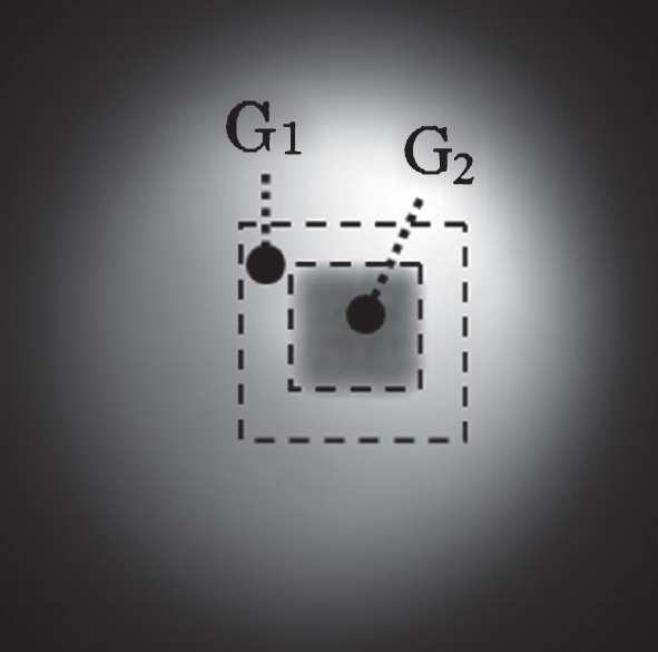
Area selections for contrast evaluation.

3 Results and discussion

The following two simulation studies were separately executed for the chromosome images with relatively high contrast or with very low contrast.

3.1 Iteration effect for the chromosome image with relatively high contrast

The noise contrast was changed from 0 to the equal level with the contrast of the diffraction fringes for the simulated projection image, that is, the ratio of the noise contrast to the contrast of diffraction fringes (it is abbreviated as “ratio K” in the following text). The iteration effect was examined for each level of the noise contrasts in Figs. 4–6. As a result, below 0.95 of the ratio K, the correction was found to be successful. Therefore the upper limit for successful correction was determined as 0.95. Image examples at each step in the simulation and the iteration procedures are shown in Fig. 4. The images in Fig. 4 correspond to those in Fig. 2 with same numbers (a – g). The X-ray illumination image (a) was captured by a projection experiment and the simulation conditions were adjusted to be the same as the projection experiment at the magnification of 329 times. The magnification was calculated as a ratio of distances from pinhole to CCD screen and to specimen position based on its optical layout. The size of the square for specimen (c) was 4μm * 4μm. The ratio K was adjusted to 0.95 or 1.00 in the projection images (f-1) and (f-2), respectively.

Fig.4

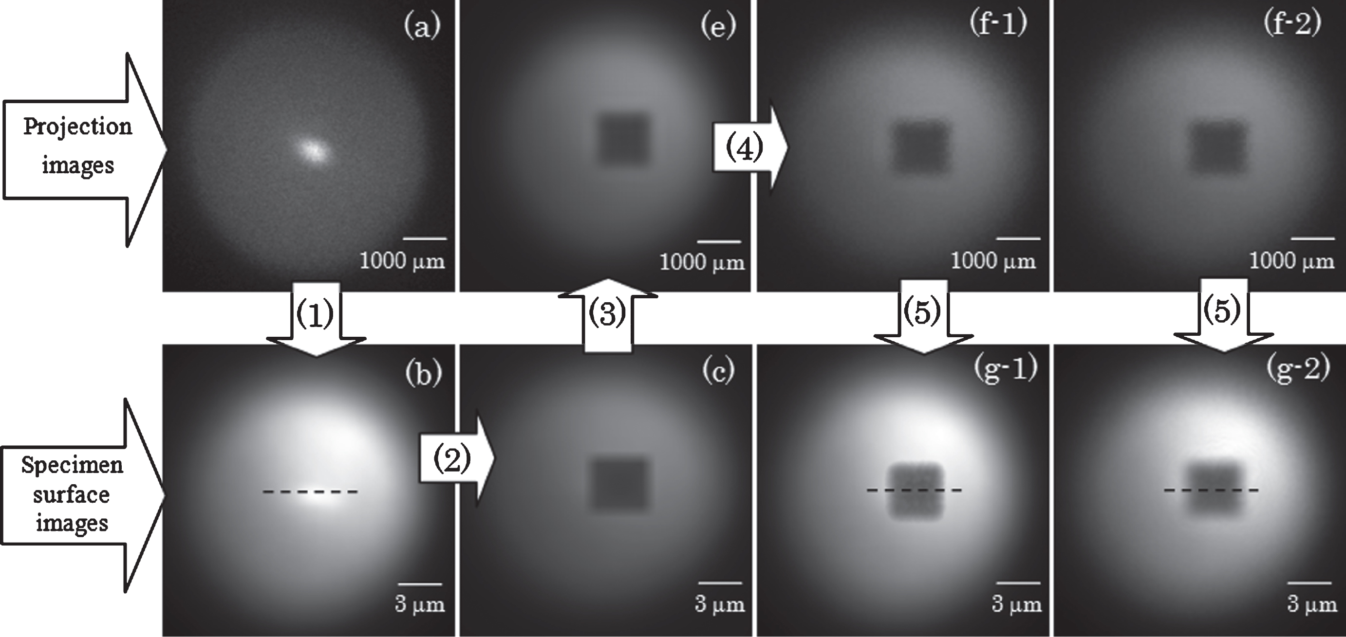
Example images for the simulation and the iteration effect on a model specimen image with high contrast. (a) X-ray illumination image in the experiments, (b) X-ray illumination image for simulation, (c) Image of model specimen (square opaque substance), (e) Projection image without noise, (f-1) Projection image with noise added (“Noise contrast”/“Contrast of diffraction fringes”≃0.95), (f-2) Projection image with noise added (“Noise contrast”/“Contrast of diffraction fringes” ≃ 1.00), (g-1) and (g-2) Corrected images, (1) Noise removal and IFT, (2) Add target figure, (3) FT, (4) Add noise, (5) Iteration.

Fig.5

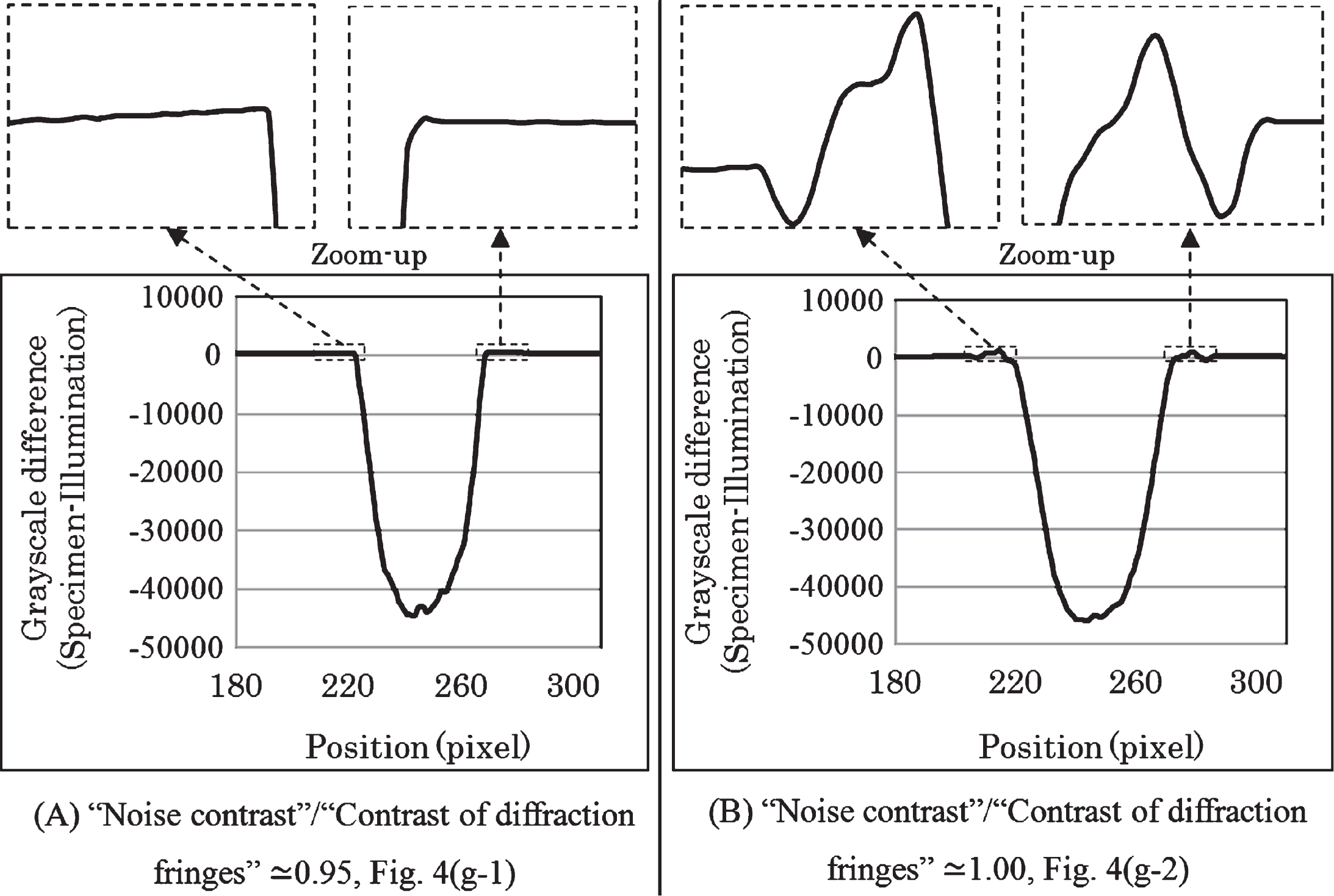
Comparision of grayscale distributions on cross-sectional lines of corrected images shown in Fig. 4 (g-1) and (g-2).

Fig.6

Relationship between noise contrast of projection image and contrast of diffraction fringes in corrected image. (Simulation results for a chromosome image with relatively high contrast) O and X: Correctable and uncorrectable regions for the ratio of the noise contrast to the contrast of the diffraction fringes, respectively.

In order to show the correction effectiveness more clearly, a comparison between grayscale distributions of Fig. 4(g-1) and (g-2) is shown in Fig. 5A and Fig. 5B. The vertical axis is difference between grayscale distributions on cross-sectional lines of the corrected image in Fig. 4(g-1) or (g-2) and the X-ray image of illumination (b). The horizontal axis is pixel position. Zoomed-up images of four edge areas on the grayscale profiles in corrected specimen images indicated by rectangles with broken lines were also shown in Fig. 5. The diffraction fringes remained in the corrected image and the edge of the specimen image was not clear in the case that the contrast was almost equal between noise and diffraction fringe (the ratio K of 1.00, Fig. 5B). On the other hand, by lowering the ratio K only 0.05, the correction was greatly improved where diffraction fringes were removed and the specimen edge was corrected clearly (Fig. 5A).

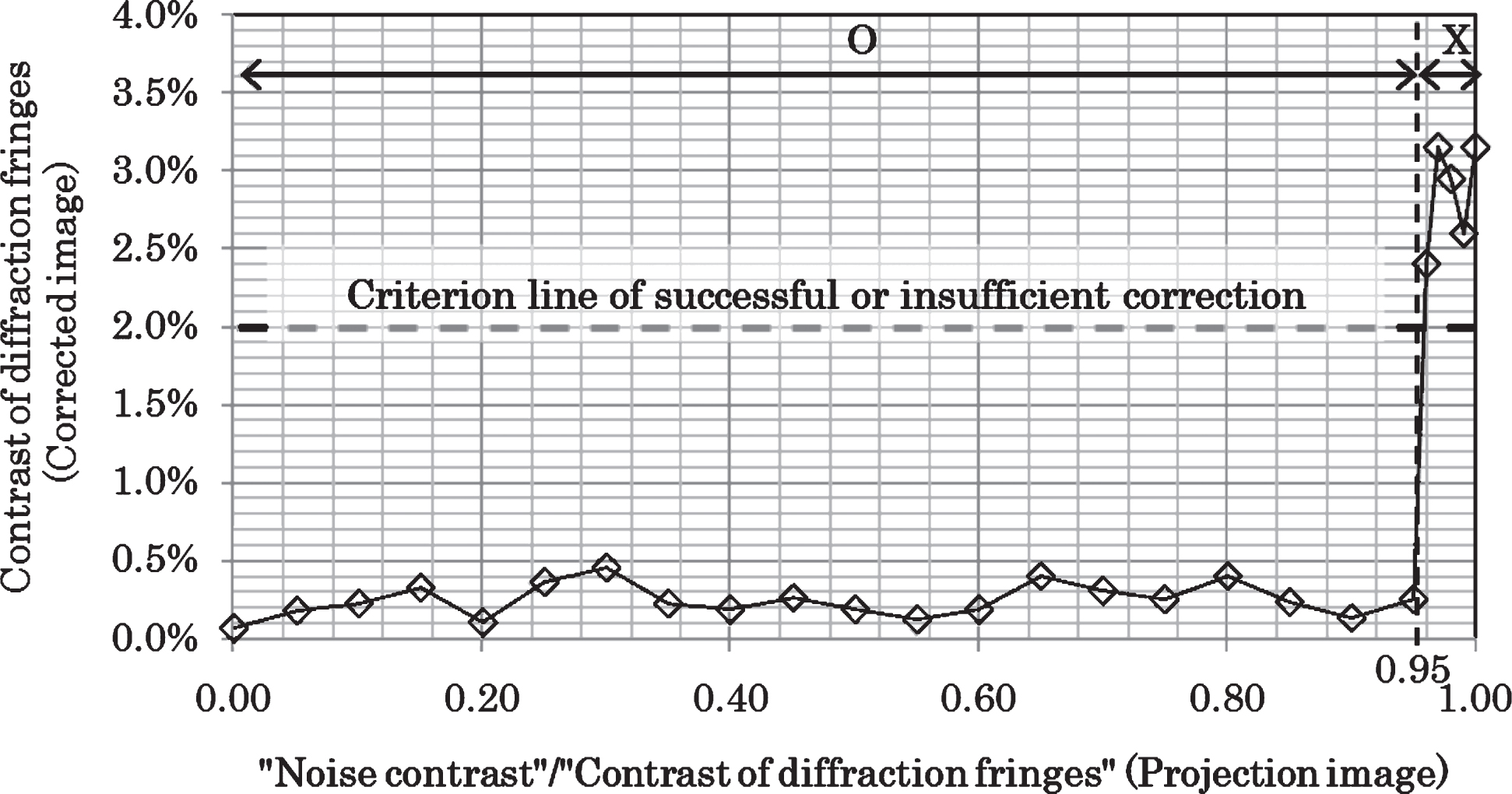
A relationship between the ratio K and the contrast of the diffraction fringes in the corrected image is shown in Fig. 6. The criterion of contrast of the diffraction fringes in the corrected image whether the correction is successful or not (2%) was described by a horizontal broken line. “O” and “X” characters show correctable and uncorrectable region of the ratio K, respectively.

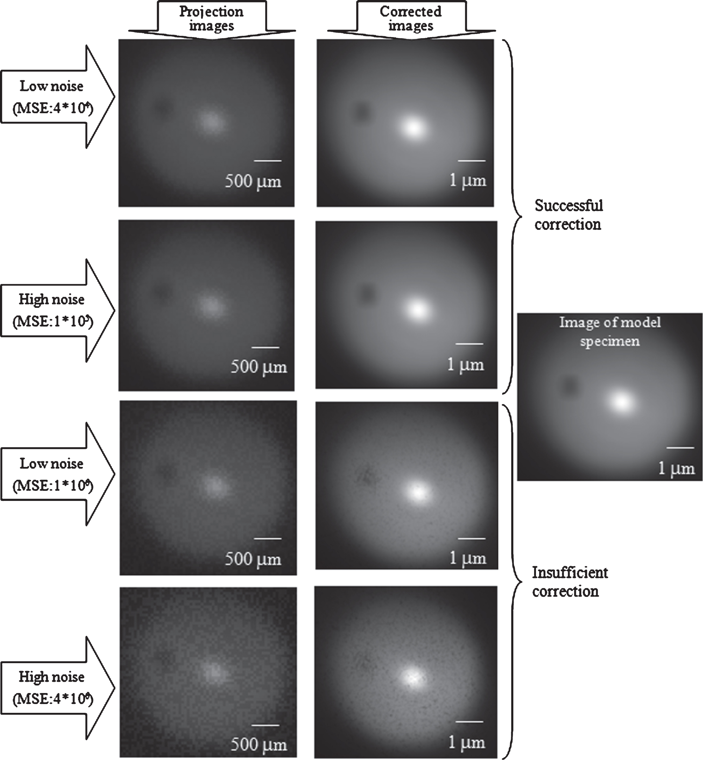
Figure 7 shows detailed results of the successful and insufficient correction. The simulated projection images and their corrected images are shown in the left and the right sides, respectively and the ratio K ranged from 0 to 1.00. Two images in the above are for the successful correction and the two images in the bottom are for the insufficient correction. An image of the model specimen prepared by simulation is also shown in the right side of the corrected images.

Fig.7

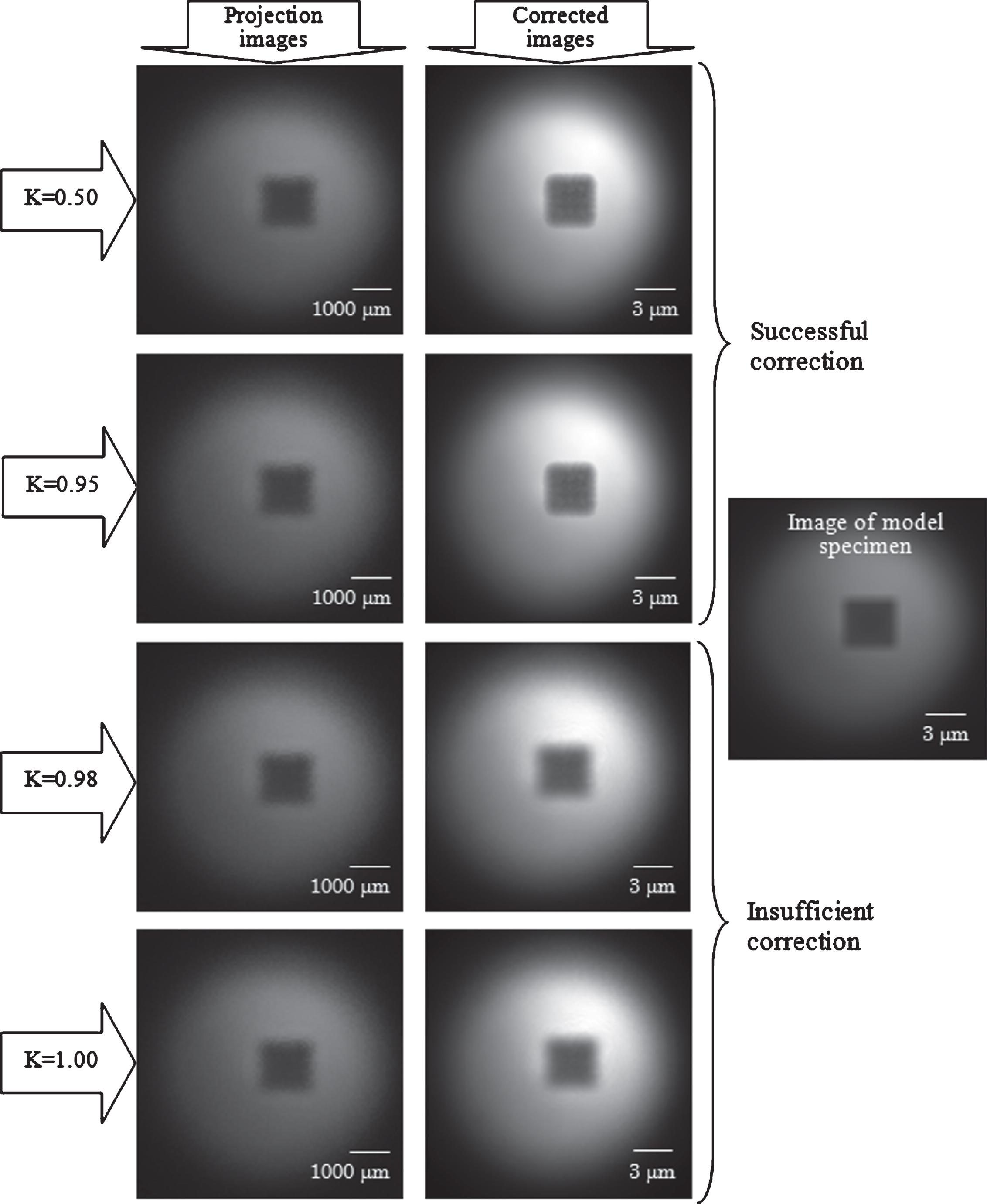
Representative results of the iteration effect on a model specimen image with high contrast. K: “Noise contrast”/“Contrast of diffraction fringe” (Projection image).

In the successfully corrected images with the ratio K of 0.95 or lower, contrast of the diffraction fringes in the corrected image was lower than 0.5% (Fig. 6) and the diffraction fringes disappeared (Fig. 7). Traced line of the specimen boundary was also equivalent to that of the model specimen for all corrected images in these cases. On the other hand, diffraction fringes remained in the corrected image where the ratio K exceeded 0.95 (Fig. 7). The contrast of the diffraction fringes in the corrected image was in the range between 2% and 3.5%. A blurred part is still visible in the image despite correction. In the case where the correction was insufficient, the X-ray diffraction fringes were considered to be interrupted by the noises with the ratio K higher than 0.95, resulting in inability to identify the diffraction fringes in the iteration procedure.

The results suggested that the diffraction fringes accompanied with the experimental projection image of chromosome would be corrected effectively by the iteration procedure when the ratio K is lower than 0.95 of the diffraction fringe contrast.

3.2 Iteration effect for the chromosome image with very low contrast

The contrast for the target on the simulated projection image was adjusted to be same as that of an experimental projection image of chromosome with the magnification of 504 times, because the chromosome morphology was captured clearly on the image. The noise MSE was adjusted from 0 to 4*10⁶.

Relationship between contrast of target in the corrected image and noise MSE on the simulated projection image was examined for model specimens with small (0.7μm * 0.7μm) and big (1.4μm * 1.4μm) sizes. The specimen sizes were decided as the maximum and minimum when magnification of 500 times is required. The result is shown in Fig. 8. The horizontal axis is noise MSE on the simulated projection image and the vertical axis is the contrast of the target on the corrected image which was evaluated by the equation (2) and normalized by the value for the noise MSE of 0. “O” and “X” characters show correctable and uncorrectable region of noise MSE, respectively (Our consideration for the judgment of correctable or uncorrectable region is explained in the second paragraph below).

Fig.8

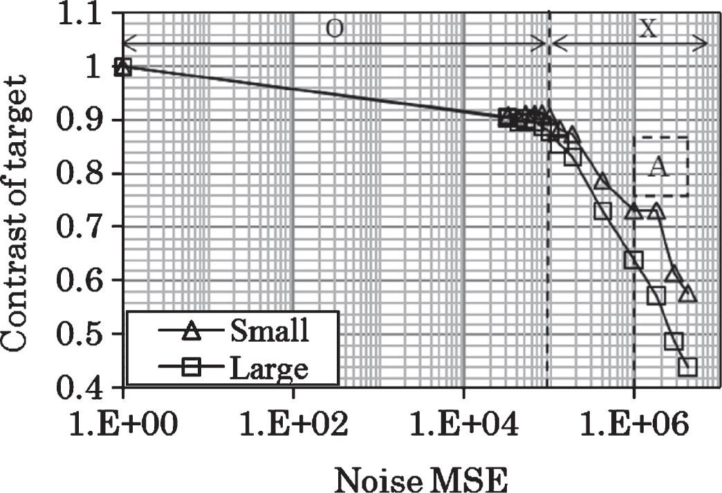
Relationship between noise MSE of projection image and contrast of target in corrected image. (Simulation results for a chromosome image with very low contrast). O: Correctable region of the noise MSE, X: Uncorrectable region of the noise MSE, A: Noise MSE for the projection image of chromosome with the magnification of 504 times.

Some representative images with high and low noise MSE are shown in Figs. 9 and 10 for the small and big specimens, respectively. In the figures, the simulated projection images and their corrected images are shown in the left and the right sides, respectively. Both images are shown for varying noise MSE ranging from 4*10⁵ to 4*10⁶. An image of the model specimen prepared by simulation is also shown in the right side of the corrected images. Two images in the above are for the successful correction and two images in the bottom are for the insufficient correction as judged from the tracing of specimen boundaries as described below. The background noise on the simulated projection images was prominent or inconspicuous for the images with high (10⁶ and 4*10⁶) or low noise MSE (4*10⁴ and 10⁵), respectively. For the corrected images with low noise MSE, traced line of the specimen boundary was equivalent to that of its projection images. It was also equivalent to the model specimen boundary. On the other hand, for the corrected image with high noise MSE, the contrast of the specimen image was lost by iteration procedure, resulting in inability to identify its morphology.

Fig.9

Representative results of the iteration effect on the projection images with very low contrast (Specimen size: 0.7μm * 0.7μm).

Fig.10

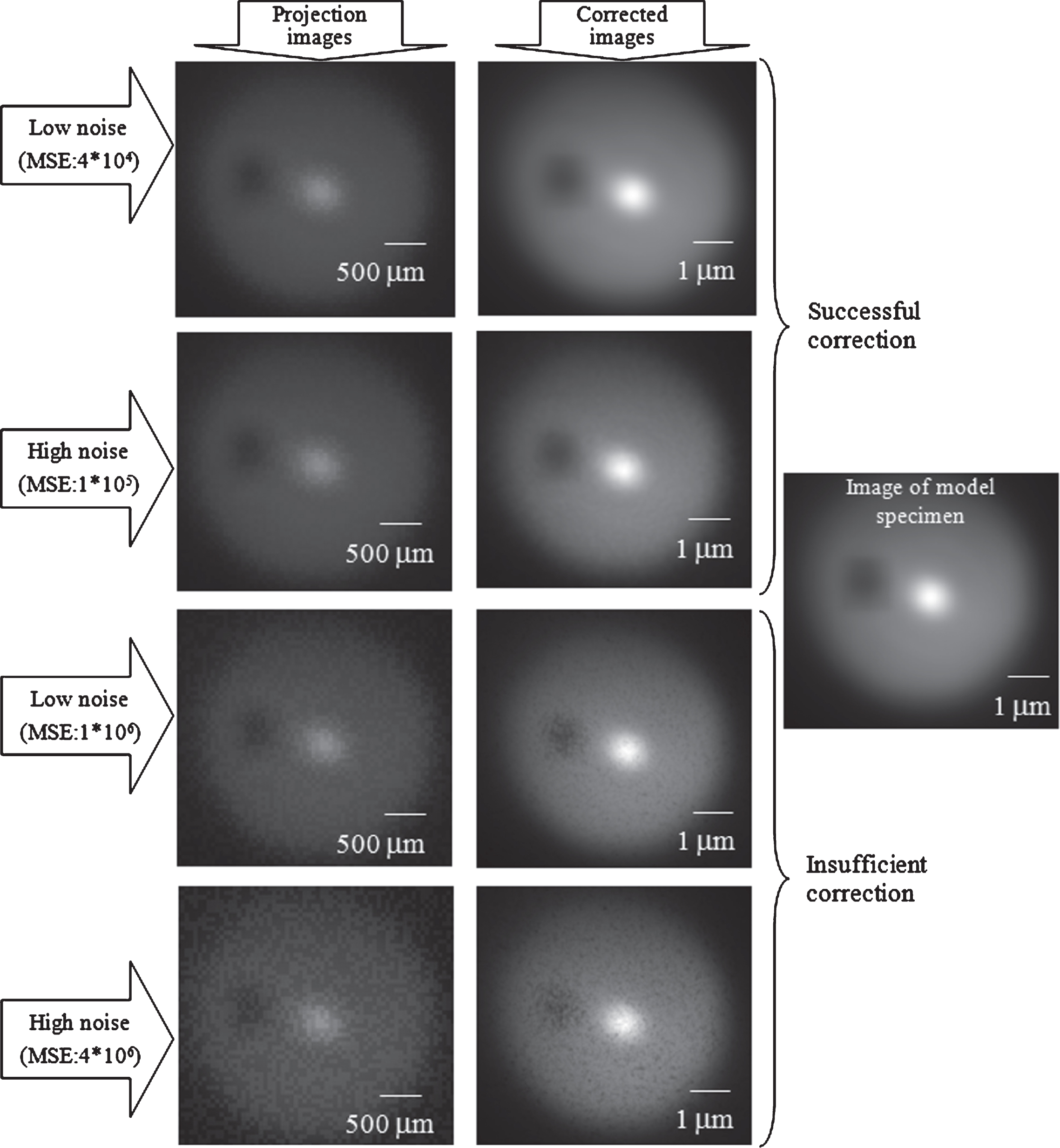
Representative results of the iteration effect on the projection images with very low contrast (Specimen size: 1.4μm * 1.4μm).

As shown in Figs. 8–10, the results were the same in the both cases of the specimen size. The image contrast decreased as the noise MSE became larger. The decreasing rate was slow until noise MSE reached about 10⁵. The contrast decreased down to about 10%, and the decrease was not observable at the noise MSE less than 10⁵. However, the decreasing rate became rapid when the noise MSE exceeded 10⁵. Therefore, we concluded that the upper limit of the noise MSE where the image was corrected effectively by iteration procedure is 10⁵ for the chromosome image. We also applied the iteration procedure to experimental projection image of the chromosome with a magnification of 504 times.

The iteration result is shown in Fig. 11. An image in the left side is the experimental projection image of chromosomes where three chromosomes are arranged side by side, and that in the right side is its corrected image. Outlines of one chromosome in each image were traced by white lines to clarify their morphology as illustrated in the left-lower side of the chromosome. As shown, the chromosome morphology became hardly identifiable after the iteration procedure. Since the noise MSE for the projection image was about 10⁶, the result is consistent with our estimation shown by “A” character in the Fig. 8.

Fig.11

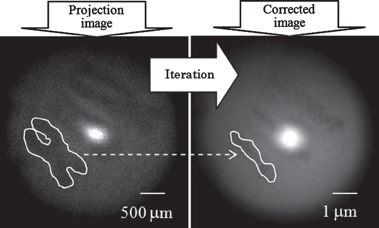
Iteration result of a chromosome image with magnification of 504 times.

One of the reasons for the high noises on the chromosome images is considered to be attributable to the scattering X-rays from debris of fragmented intracellular components of a specimen. A simple and effective washing of the specimen using fresh fixative has been adopted to clean up the debris with few loss of the chromosomes. In the future project the effectiveness of washing specimens is needed to check. Also, based on the evaluation obtained in this study, images should be captured with noises less than their upper limits after examining the noise on the image during experiments and optimizing the projection conditions. Moreover, development of new noise removal methods in image processing while keeping target morphology would be essential for better imagecorrection.

4 Summary

This study confirmed that the background noises on the projection image of chromosome affected significantly the iteration results and evaluated the upper limits of the noise within which the projection images were corrected effectively by the iteration procedure. The results are summarized as follows:

For chromosome images with relatively high contrast, where diffraction fringes are significantly observed, contrast ratio of the noise to the diffraction fringes were evaluated and the upper limit of the ratio was determined to be 0.95.

For chromosome images with very low contrast, noise MSE was introduced and the upper limit of the noise MSE was 10⁵.

The methods of the simulation and the noise evaluation developed here is useful for image processing where background noises cannot be ignored compared with specimen images.

Footnotes

Acknowledgments

The work was performed at the Photon Factory under the application numbers 2010G065, 2012G120 and 2014G148. We would like to thank the Photon Factory staff, Dr. Yoshinori Kitajima. We also thank Dr. Kunio Shinohara, Dr. Toshio Honda and Dr. Keiji Yada for their helpful discussion and advice.

References

Weigert

, Porat-Shliom

and Amornphimoltham

, Imaging cell biology in live animals: Ready for prime time, Journal of Cell Biology 201(7) 2013, 969–979.

Kirz

, Jacobsen

and Howells

, Soft X-ray microscopes and their biological applications, Quarterly Reviews of Biophysics 28 (1995), 33–130.

Williams

, Zhang

, Jacobsen

, Kirz

, Lindaas

, Van’t Hof

and Lamm

S.S.

, Measurements of wet metaphase chromosomes in the scanning transmission X-ray microscope, Journal of Microscopy 170(Pt.2) (1993), 155–165.

Shinohara

and Ito

, Radiation damage in soft X-ray microscopy of live mammalian cells, Journal of Microscopy 161(Pt 3) (1991), 463–472.

Takeichi

, Inami

, Suga

, Ueno

, Kishimoto

, Takahashi

and Ono

, Development of a compact scanning transmission X-ray microscope, Journal of Physics: Conference Series (IOP) 502 (2014), 0112009.

McDermott

, Le Gross

M.A.

and Larabell

C.A.

, Visualizing cell Architecture and molecule location using soft X-ray tomography and correlated cryo-light microscopy, Annual Review of Physical Chemistry 63 (2012), 225–239.

Müller

W.G.

, Heymann

J.B.

, Nagashima

, Guttmann

, Werner

, Rehbein

, Schneider

, McNally

J.G.

, Towards an atlas of mammalian cell ultrastructure by cryo soft X-ray tomography, Journal of Structural Biology 177 (2012), 179–192.

Kinjo

, Shinohara

, Ito

, Nakano

, Watanabe

, Horiike

, Kikuchi

, Richardson

M.C.

and Tanaka

K.A.

, Direct imaging in a water layer of human chromosome fibers composed of nucleosomes and their higher-order structures by laser-plasma X-ray contact microscopy, Journal of Microscopy 176 (1994), 63–74.

Shinohara

, Nakano

, Kinjo

and Watanabe

, Fine structure of unstained human chromosome fibres dried with no fixative as observed by X-ray contact, Journal of Microscopy 158 (1990), 335–342.

10.

Kirz

and Rarback

, Soft X-ray microscopes, AIP Review of Scientific Instruments 56(1) (1985), 1–13.

11.

Shinohara

, Ito

, Honda

, Yoshimura

and Yada

, Development of an X-ray projection microscope using synchrotron radiation, AIP Conference Proceedings 507(1) (2000), 346.

12.

Mayo

S.C.

, Miller

P.R.

, Wilkins

S.W.

, Davis

T.J.

, Gao

, Gureyev

T.E.

, Paganin

, Parry

D.J.

, Pogany

and Stevenson

A.W.

, Quantitative X-ray projection microscopy: Phase-contrast and multi-spectral imaging, Journal of Microscopy 207(2) (2002), 79–96.

13.

Yada

and Takahashi

, Projection X-ray microscope observation of biological samples, X-ray Microscopy in Biology and Medicine, Japan Science Society Press, Tokyo/Springer-Verlag, Berlin, 1990, pp. 203–212.

14.

Shiina

, Suzuki

, Honda

, Ito

, Kinjo

, Yoshimura

, Yada

and Shinohara

, Fresnel diffraction correction by phase-considered iteration procedure in soft X-ray projection microscopy, Journal of Physics: Conference Series (IOP) 186 (2009), 120591–120593.

15.

Chikwendu

S.C.

, Non-linear wave propagation solutions by Fourier transform perturbation, Int J Non-linear Mechanics 16 (1981), 117–128.

16.

Cooley

J.W.

and Turkey

J.W.

, An algorithm for the machine calculation of complex Fourier series, Mathematics of Computation 19(90) (1965), 297–301.

17.

Robertson

J.M.

, X-ray analysis and application of Fourier series methods to molecular structure, Reports on Progress in Physics 4 (1937), 332–367.

18.

Jamsranjav

, Shiina

, Kuge

, Kinjo

, Nakamura

, Shinohara

and Ito

, Effect of contrast enhancement prior to iteration procedure on image correction for soft X-ray projection microscopy, AIP Conference Proceedings 1696 (2016), 0200371–0200375.

19.

Al-amri

S.S.

, Kalyankar

N.V.

and Khamitkar

S.D.

, Linear and non-linear contrast enhancement image, IJCSNS International Journal of Computer Science and Network Security 10(2) (2010), 139–143.

20.

Attwood

, Soft X-rays and extreme ultraviolet radiation, Principles and applications, Cambridge University Press, Cambridge, 1999.

21.

Rautenstrauß

and Liehr

(eds.), FISH technology, Springer lab manual, Springer Verlag Berlin Heidelberg, 2002, pp. 73–81.

22.

Bohren

C.F.

and Clothiaux

E.E.

, Fundamentals of atmospheric radiation, Wiley-VCH Verlag GmbH & Co. KGaA, Fedral Republic of Germany, 2006.

23.

Gonzalez

R.C.

and Woods

R.E.

, Digital image processing, Third edition, Pearson Education, Inc., New Jersey, 2008.

24.

Peli

, Contrast in complex images, Journal of the Optical Society of America A 7(10) (1990), 2032–2040.