Data correlation based noise level estimation for cone beam projection data

Abstract

BACKGROUND:

In regularized iterative reconstruction algorithms, the selection of regularization parameter depends on the noise level of cone beam projection data.

OBJECTIVE:

Our aim is to propose an algorithm to estimate the noise level of cone beam projection data.

METHODS:

We first derived the data correlation of cone beam projection data in the Fourier domain, based on which, the signal and the noise were decoupled. Then the noise was extracted and averaged for estimation. An adaptive regularization parameter selection strategy was introduced based on the estimated noise level. Simulation and real data studies were conducted for performance validation.

RESULTS:

There exists an approximately zero-energy double-wedge area in the 3D Fourier domain of cone beam projection data. As for the noise level estimation results, the averaged relative errors of the proposed algorithm in the analytical/MC/spotlight-mode simulation experiments were 0.8%, 0.14% and 0.24%, respectively, and outperformed the homogeneous area based as well as the transformation based algorithms. Real studies indicated that the estimated noise levels were inversely proportional to the exposure levels, i.e., the slopes in the log-log plot were -1.0197 and -1.049 with respect to the short-scan and half-fan modes. The introduced regularization parameter selection strategy could deliver promising reconstructed image qualities.

CONCLUSIONS:

Based on the data correlation of cone beam projection data in Fourier domain, the proposed algorithm could estimate the noise level of cone beam projection data accurately and robustly. The estimated noise level could be used to adaptively select the regularization parameter.

Keywords

Fourier domain cone beam projections noise level estimation

1 Introduction

X-ray cone beam computed tomography (CBCT) has been applied in various scenarios, such as patient setup in radiation therapy [1] and maxillofacial region visualization in dentistry [2]. Despite the successful applications, image noise still remains a major issue in low-dose CBCT. A great effort has been devoted to image noise reduction(e.g., [3 –7]). Specifically, regularized iterative reconstruction algorithms could produce superior image qualities with noisy projection data, and hence have become more and more popular(e.g., [5 –9]).

Despite the superiority of the regularized iterative algorithms, the effectiveness of a regularized method strongly depends on the selection of a suitable regularization parameter [10, 11]. And Many literature demonstrated that the selection of the regularization parameter λ is highly correlated with the noise level ɛ of the noisy projection data p defined as $ɛ = | | p^{0} - p | |_{2}^{2},$ (1) where p⁰ is the noise-free projection data. For example, the discrepancy principle determines a concrete value of λ by enforcing the realized residual to be compatible with a given noise level ɛ [11]. By introducing a model function to solve the Morozov equation, the Morozov discrepancy principle states that a good λ is supposed to be the value that could make the error due to the regularization is equal to the noise level ɛ [12]. Kazufumi Ito et al. proposed a novel rule to determine the regularization parameter based on the balancing principle [13], where a constant factor related with the noise level ɛ should be pre-determined. Despite the theoretical developments of the regularization parameter selection strategies, it seems that few of them are applied in practice. One of the reasons may be that these methods require the knowledge of the noise level ɛ, which is usually unavailable in practice. Thus, to solve this problem, in this work, we will propose an algorithm to estimate the noise level ɛ of cone beam projection data, so as to facilitate the regularized iterative reconstruction algorithms.

According to our best knowledge, most of the existing noise level estimation algorithms are designed for the natural scene images, and thus here we would provide a brief review on them. Generally speaking, they could be classified into four categories, i.e., homogeneous areas based, filter based, transformation based and patch based. Assuming that the noise of any pixel is independently identically distributed (i.i.d.), the homogeneous areas based algorithms try to pre-classify some homogeneous areas in the image, based on which, the constant component is subtracted and then the rest could be employed to calculate the noise level [14, 15]. By calculating the difference between the original noisy image and the associated low-pass filtered image, and then removing the residual edges with an edge detection algorithm, the filter based algorithms estimate the noise level directly from the above processed results [16, 17]. The transformation based algorithms first separate the signal and the noise via transformation such as wavelet transform or discrete cosine transform, and then estimate the noise level in some specified band, such as the high frequency domain [18, 19]. In the patch based algorithms which also suppose that the noise of any pixel is i.i.d., the image would be decomposed into a large amount of patches, from which, those patches with small variance will be selected for the noise level estimation [20].

As stated above, the homogeneous areas based and the patch based algorithms require that the noise should be i.i.d., which however does not hold in the context of cone beam projection data, where the noise components after log transform are supposed to follow Gaussian distribution with ray-dependent variance [21, 22]. The filter based algorithms may cause a biased noise level estimation if there still exist image contents in the difference result. As for the transformation based algorithms, significant over-estimates of the noise level may be achieved concerning the potential image structures in the high frequency domain. Therefore, so far it still remains a challenge to accurately estimate the noise level ɛ of the cone beam projection data.

In this work, we will propose a new algorithm to estimate the noise level of cone beam projection data and demonstrate its practical utility on adaptive regularization parameter selection. Specifically, by investigating the data correlation of cone beam projection data in the 3D Fourier domain, we could theoretically decouple the signal and the noise. As a result, the pure noise components could be extracted to enable the estimation of the noise level ɛ. Finally, an adaptive noise level driven regularization parameter selection strategy is introduced to demonstrate its practical utility. In the following section, we will first derive the data correlation of cone beam projection data in the 3D Fourier domain, and detail the proposed noise level estimation algorithm. Then we will introduce our parameter selection strategy based on the estimated noise level. In Section 3, experimental results will be presented to validate the efficacy of the proposed algorithm under different geometry configurations, including ideal geometry, spotlight-mode, short-scan mode and half-fan mode. Finally, we will discuss and conclude the whole paper in Sections 4 and 5, respectively.

2 Methods and materials

2.1 Data correlation of CT sinogram in 2D Fourier domain

CT sinogram exhibits a unique property in its 2D Fourier domain, namely, there exists an approximately zero-energy double-wedge area. Its theoretical formalism has been introduced in an earlier paper [10, 11]. Here, we will briefly present this data correlation for completeness. Equal-spaced fan beam geometry with a circle orbit will be used as an example.

Let us consider an object composed of a delta function point, which located at distance r from the origin and at angle φ with respect to the x-axis. It could be denoted by δ (r, φ) in the polar coordinate system. Then, the Radon transform of δ (r, φ) can be expressed as $p^{0} (u, β) = δ (u - u_{0} (β)),$ (2) where $u_{0} (β) = (L + D) \frac{\frac{r}{L} cos (φ - β)}{1 - \frac{r}{L} sin (φ - β)},$ (3) here, u represents the local coordinate on the line detector array, β, L and D denote the view angle, the source-axis-distance and the axis-detector-distance, respectively.

By taking 2D Fourier transform to p⁰ (u, β), one has $\begin{matrix} P (q, k) & = & \frac{1}{2 π} \int_{- π}^{π} \int_{- \infty}^{+ \infty} δ (u - u_{0} (β)) e^{- i (qu + k β)} d u d β \\ = & \frac{1}{2 π} e^{- ik (φ + \frac{π}{2})} \int_{- π}^{π} e^{- i [q (L + D) \frac{\frac{r}{L} sin β}{1 + \frac{r}{L} cos β} - k β]} d β \\ \approx & e^{- jk (φ + \frac{π}{2})} J_{k} ((k - q (L + D)) \frac{r}{L}), \end{matrix}$ (4) where q, k are the angular frequency variables associated with u and β, respectively. J_k (·) is a Bessel function of the first kind of order k. Note that the approximation made in Equation (4) was achieved intuitively and validated empirically as stated in the reference [23].

It is noted that a Bessel function rapidly decreases to zero as the argument becomes less than the order. As a result, P (q, k) ≈0 for those angular frequencies such that $| \frac{k}{k - q (L + D)} | > \frac{r}{L} .$ (5)

This indicates that there exists an approximately zero-energy double-wedge area in the 2D Fourier domain whose boundaries are defined by Equation (5).

2.2 Data correlation of cone beam projections in 3D Fourier domain

Motivated by the data correlation of CT sinogram in 2D Fourier domain, we will explore whether a similar zero-energy double-wedge area exists in the 3D Fourier domain of cone beam projection data.

Suppose there exists an object composed of a delta function point δ (r, θ, φ), where r is the distance from the origin, θ and φ correspond to the polar angle and the azimuthal angle, respectively. After cone beam transform, the resultant cone beam projections p⁰ (u, v, β) can be expressed as

$p^{0} (u, v, β) = δ (u - u_{0} (β)) δ (v - v_{0} (β)),$ where $u_{0} (β) = (L + D) \frac{\frac{r}{L} cos θ cos (φ - β)}{1 - \frac{r}{L} cos θ sin (φ - β)},$ $v_{0} (β) = (L + D) \frac{\frac{r}{L} \sin θ}{1 - \frac{r}{L} \cos θ \sin (ϕ - β)}$

Again, β, L and D correspond to the view angle, the source-axis-distance and the axis-detector-distance, respectively. (u, v) are the 2D coordinates in the detector plane.

Taking 3D Fourier transform to the cone beam projections p⁰ (u, v, β) yields $\begin{matrix} P (q, ξ, k) & = & \int_{- π}^{π} \int_{- \infty}^{+ \infty} \int_{- \infty}^{+ \infty} δ (u - u_{0} (β)) δ (v - v_{0} (β)) e^{- i (qu + ξ v + k β)} d u d v d β \\ = & \int_{- π}^{π} e^{- i {q (L + D) \frac{\frac{r}{L} cos θ sin β^{'}}{1 + \frac{r}{L} cos θ cos β^{'}} + ξ (L + D) \frac{\frac{r}{L} sin θ}{1 + \frac{r}{L} cos θ cos β^{'}} + k (- β^{'} + φ + \frac{π}{2})}} d β^{'}, \end{matrix}$ (6) where q, ξ, k are the angular frequency variables associated with u, v, β, respectively. Here we have changed the dummy variable β to -β′ + φ + π/2.

It is noted that for a typical CBCT geometry setting, $1 \approx 1 - (\frac{r}{L} cos θ cos β)^{2}$ , i.e., $\frac{1}{1 + \frac{r}{L} cos θ cos β} \approx 1 - \frac{r}{L} cos θ cos β$ . Here, we would like to take typical CBCT geometry used in radiation therapy, such as the on board imager (OBI) integrated in a Varian’s LINAC (Varian Medical System, Palo Alto, CA) as the example for numerical validation. Generally speaking, suppose a typical patient has a radius r ≈ 15 cm, the source-axis-distance L ≈ 100 cm. In the case that θ = 0 and β = 0, the approximation error between 1 and $1 - (\frac{r}{L} cos θ cos β)^{2}$ is about 2.25%, which suggests the reasonableness of the above approximation.

Now replace the dummy variable β′ with β for simplicity, and then plug the above approximation into the second term in the exponential function in Equation (6), one has

$\begin{matrix} P (q, ξ, k) & \approx & e^{- i ξ (L + D) \frac{r}{L} sin θ} e^{- ik (φ + π / 2)} \\ \times \int_{- π}^{π} e^{- i {q (L + D) \frac{\frac{r}{L} cos θ sin β}{1 + \frac{r}{L} cos θ cos β} - ξ (L + D) (\frac{r}{L})^{2} sin θ cos θ cos β - k β}} d β \\ \approx & e^{- i ξ (L + D) \frac{r}{L} sin θ} e^{- ik (φ + π / 2)} \\ \times \int_{- π}^{π} e^{- i {q (L + D) \frac{\frac{r}{L} cos θ sin β}{1 + \frac{r}{L} cos θ cos β} - k β}} e^{iz cos β} d β, \end{matrix}$ (7) where z = ξ (L + D) δ² sin θ cos θ and $δ = \frac{r}{L}$ . Comparing Equation (7) with Equation (4), one could find that Equation (7) also could be approximated with a Bessel function of the first kind if without e^izcosβ inside the integration in Equation (7), and thus resulting in a similar zero-energy double-wedge area in the 3D Fourier domain.

Now we would like to focus on exploring the impact of e^izcosβ on the approximation of the Bessel function. One can expand e^izcosβ on the basis of the Bessel functions of the first kind as

$\begin{matrix} e^{iz cos β} & = & \sum_{n = - \infty}^{+ \infty} i^{n} J_{n} (z) e^{in β} \\ = & J_{0} (z) + \sum_{n = 1}^{+ \infty} i^{n} J_{n} (z) e^{in β} + \sum_{n = 1}^{+ \infty} i^{n} (- 1)^{2 n} J_{n} (z) e^{- in β} \\ = & J_{0} (z) + 2 \sum_{n = 1}^{+ \infty} i^{n} J_{n} (z) cos (n β) . \end{matrix}$ (8)

Here, we have utilized the property J_-n (x) = (-1) ⁿJ_n (x). It is shown that the first term J₀ (z) is independent on the integral variable β, and hence could be taken out from the integration in Equation (7). The second term correlates with cos(nβ) whose period is $\frac{2 π}{n}$ . As n increases, the period would decrease and the corresponding frequency of cos(nβ) would increase. Therefore, it is expected that the second term in Equation (8) would approximate zero when performing summation, considering that the second term contains many high frequency components of β. If this assumption holds, it is reasonable to approximate e^izcosβ with J₀ (z). However, it is found experimentally that the term e^izcosβ contributes additional effects except J₀ (z), which means that the second term in Equation (8) could not be approximated with zero simply. For now, it is not a trivial task to quantitatively and mathematically demonstrate how to take e^izcosβ out from the integration in Equation (7). Fortunately, according to our experiments, we find that the term e^izcosβ does not affect the Bessel function approximation. On the other hand, in order to estimate the noise level of cone beam projection data, we just need to decouple the signal and the noise. Therefore, an exact mathematical expression may be not necessary. Considering this purpose, in this work, we will temporally regard the impact of e^izcosβ inside the integration in Equation (7) as an unknown function g. According to Equation (4) and our derivation, we could approximate the Fourier transform of the cone beam projection data as follows

$P (q, ξ, k) \approx g e^{- i [k (φ + \frac{π}{2}) + ξ (L + D) \frac{r}{L} sin θ]} J_{k} ((k - q (L + D)) \frac{r}{L} cos θ) .$ (9)

Based on the fact that Bessel function tends to zero rapidly when the argument becomes less than the order, Equation (9) reveals that there also exists an approximately zero-energy double-wedge area in the 3D Fourier domain of cone beam projection data. In other words, P (q, ξ, k) ≈0 for all the frequency components (q, ξ, k) satisfying $| \frac{k}{k - q (L + D)} | > \frac{r}{L} cos θ .$ (10)

Equation (10) is for an object composed of a delta function. A real object could be considered as a linear combination of multiple delta functions, so does the Fourier domain of the real object. As indicated by the arrow in Fig. 1(b), the approximately zero-energy double-wedge area could be clearly observed from the 3D Fourier domain of the cone beam projection data of a real object.

Fig.1

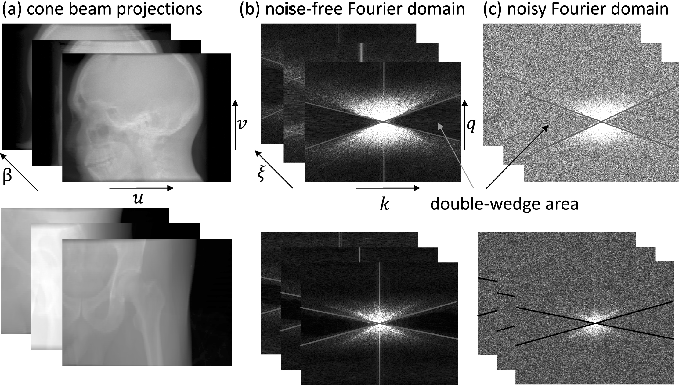
Fourier domains of cone beam projection data. The first and the second rows correspond to the head-neck and the prostate sections’ cone beam projection data, respectively. Column (a) is the cone beam projection data, columns (b) and (c) are the noise-free and noisy versions of the 3D Fourier domain, respectively. q, ξ, k are the angular frequency variables associated with u, v, β, respectively. The arrows indicate the approximately zero-energy double-wedge area.

Note that when θ = 0, the cone beam projections will be reduced to the 2D CT sinogram. By setting θ = 0 in Equation (7), one gets

$\begin{matrix} P (q, ξ, k) & \approx & e^{- ik (φ + π / 2)} \int_{- π}^{π} e^{- i {q (L + D) \frac{\frac{r}{L} sin β}{1 + \frac{r}{L} cos β} - k β}} d β \\ \approx & e^{- ik (φ + \frac{π}{2})} J_{k} ((k - q (L + D)) \frac{r}{L}), \end{matrix}$ (11) which is exactly the equal-spaced fan beam case, as presented in Equation (4).

Moreover, when L tends to infinity, the cone beam geometry will approach the 3D parallel projection geometry. In this case, Equation (7) becomes $P (q, ξ, k) = e^{- i ξ (L + D) \frac{r}{L} sin θ} e^{- ik (φ + \frac{π}{2})} J_{k} (q (L + D) \frac{r}{L} cos θ) .$ (12)

2.3 Characterization of noise in the Fourier domain

In this section, we will present the characteristics of the Fourier transformed noise, which would be used for the development of the proposed noise level estimation algorithm. For simplicity, let us assume that the noise are acquired at pixels with discrete coordinates. We denote the noise associated with the projection data p⁰ (u, v, β) by n (u, v, β), which follows zero-mean Gaussian distribution with ray-dependent variance σ² (u, v, β) that has been validated experimentally previously [21]. Using the discrete Fourier transform, the noise in the Fourier domain can be expressed as $N (q, ξ, k) = \sum_{u} \sum_{v} \sum_{β} n (u, v, β) e^{- i (qu + ξ v + k β)},$ where N (q, ξ, k) is a zero-mean complex Gaussian random variable. Further assuming that the noise do not have correlations with each other, i.e., E [n (u, v, β) n (u′, v′, β′)] = σ² (u, v, β) δ (u - u′, v - v′, β - β′), where E [·] represents the expectation of a random variable, it follows that

$\begin{matrix} E [∥ N (q, ξ, k) ∥_{2}^{2}] & = & E [N (q, ξ, k) \times \bar{N (q, ξ, k)}] \\ = & \sum_{u} \sum_{v} \sum_{β} σ^{2} (u, v, β), \end{matrix}$ (13) where $\bar{N (q, ξ, k)}$ denotes the complex conjugate of N (q, ξ, k). Equation (13) indicates that the Fourier transformed noise is uniformly distributed in terms of that for any point of the Fourier transformed noise, the expectation of the square of the amplitude is the same, and equals to ∑_u∑_v∑_βσ² (u, v, β). This could be clearly observed from the noise components in Fig. 1(c).

2.4 Data correlation based noise level estimation

Equation (9) indicates that there exists an approximately zero-energy double-wedge area in the 3D Fourier domain of cone beam projections. Equation (13) suggests that the transformed noise is uniformly distributed. As a result, if we perform discrete Fourier transform on the noisy projection data, the signal and the noise would be well-decoupled in the above double-wedge area which could be used to estimate the noise level, as indicated by Fig. 1.

Let us denote the noisy cone beam projection by p (u, v, β), and the noise-free counterpart by p⁰ (u, v, β), respectively. Consequently, p (u, v, β) = p⁰ (u, v, β) + n (u, v, β), where n (u, v, β) is the associated noise. According to Equation (13), one has

$\begin{matrix} ɛ & = & \sum_{u} \sum_{v} \sum_{β} (p (u, v, β) - p^{0} (u, v, β))^{2} \\ \approx & E [\sum_{u} \sum_{v} \sum_{β} (p (u, v, β) - p^{0} (u, v, β))^{2}] \\ \approx & \sum_{u} \sum_{v} \sum_{β} σ^{2} (u, v, β) \\ \approx & E (| | N (q, ξ, k) | |_{2}^{2}) . \end{matrix}$ (14)

Equation (14) suggests that the noise level can be approximated with the expectation of the square of the amplitude of the Fourier transformed noise in any point. Moreover, because the Fourier transformed noise is uniformly distributed according to Equation (13), the above expectation $E (| | N (q, ξ, k) | |_{2}^{2})$ , or the noise level ɛ, could be faithfully estimated with an ensemble averaging by extracting the Fourier transformed noise reside in the double-wedge area, as indicated by the arrows in Fig. 1.

The algorithm flowchart is illustrated in Fig. 2. In details, as indicated by Equation (10), the theoretical boundaries of the double-wedge area are independent on variable ξ, which suggests that the boundaries of any q - k plane could be straightforwardly generalized to any other planes. Therefore, we first perform 3D Fourier transform on the cone beam projection data, and calculate the maximum intensity projection (MIP) of the 3D Fourier domain along ξ direction, whose edge could be generated with the Canny method [24, 25]. Then one could locate the boundaries of the zero-energy double-wedge area with a Hough transform based line detector [26]. The above detected boundaries could be extended to the 3D domain by stacking it along the ξ direction, and hence construct the 3D double-wedge boundaries. Finally, the noise level ɛ could be estimated by performing an ensemble averaging with the Fourier transformed noise inside the above detected area.

Fig.2

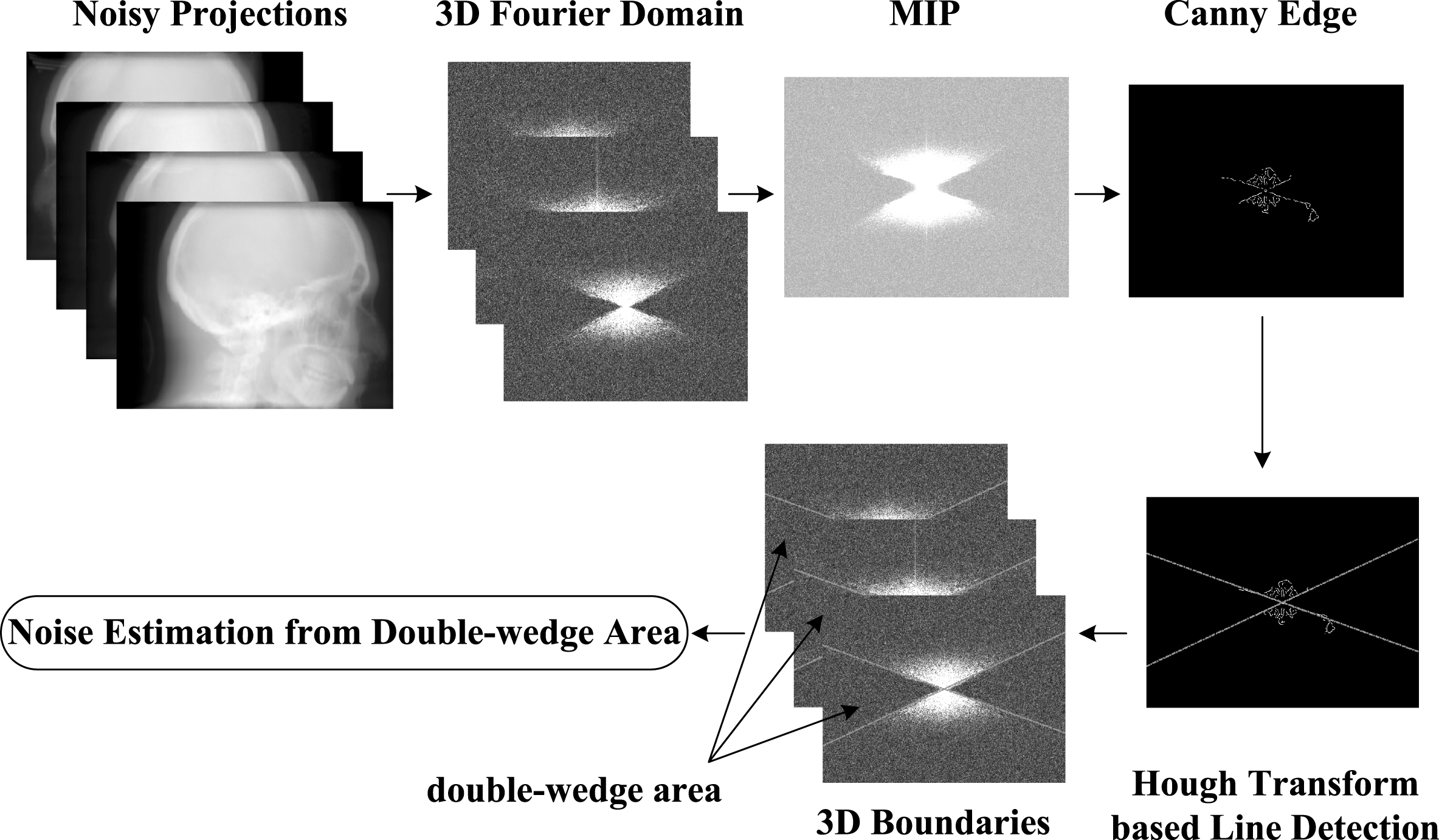
Workflow of the proposed noise level estimation algorithm.

Here it is worth mentioning that only the data inconsistencies resulting from the stochastic noise are considered in the estimated noise level ɛ, while other data inconsistencies including the scatter and the beam hardening effects are considered as part of the noise-free projection data p⁰ (u, v, β).

2.5 Noise level driven regularization parameter selection

To demonstrate the practical utility of our estimated noise level ɛ, we propose a new adaptive regularization parameter selection strategy which is driven by the estimated noise level ɛ. We will first formulate the iterative reconstruction framework, and then describe our adaptive selection strategy.

Generally speaking, regularized iterative reconstruction is equivalent to maximize the following posterior: $P (μ | p) = \frac{P (p | μ) P (μ)}{P (p)},$ (15) where p and μ denote the projection data and the reconstructed image, respectively.

In this work, we adopt the Gaussian model for the noise of the projection data [21], i.e., the noise of each ray is independent and follows a zero-mean Gaussian distribution with ray-dependent variance $σ_{i}^{2}$ , i denotes the ith ray (For simplicity, here we use i to index the ray instead of u, v, β). Suppose A denotes the system matrix, then we have $P (p | μ) \propto \prod_{i} e^{- \frac{([A μ]_{i} - p_{i})^{2}}{σ_{i}^{2}}} .$ (16)

Regarding the prior information P (μ), it represents some kind of prior distribution of μ depending on the selection of the regularizer. Inspired by the development of the compressive sensing [27], sparsity-promotion based regularizers have become popular, such as total variation (TV) minimization based regularizer [5]. In this work, we will also take TV as an example. In fact, TV based regularizer supposes that each point in the gradient map $| | ▿ μ | |_{1}^{1}$ follows a Laplacian distribution with variance α, i.e., $P (μ) \propto e^{- \frac{| | ▿ μ | |_{1}^{1}}{α}} .$ (17)

Substituting Eqs. (16) and (17) into Equation (15), performing negative log transform and ignoring the constants, the loss function could be formulated as: $L (μ) = \sum_{i} \frac{([A μ]_{i} - p_{i})^{2}}{σ_{i}^{2}} + \frac{1}{α} | | ▿ μ | |_{1}^{1} .$ (18)

As presented in Section 2.4, noise level $ɛ = \sum_{i} σ_{i}^{2}$ . Therefore, we could normalize $σ_{i}^{2}$ as $σ_{i}^{' 2} = \frac{σ_{i}^{2}}{ɛ}$ . With the normalized variance, the modified loss function could be written as:

$\begin{matrix} L^{'} (μ) & = & \sum_{i} \frac{([A μ]_{i} - p_{i})^{2}}{σ_{i}^{' 2}} + \frac{ɛ}{α} | | ▿ μ | |_{1}^{1} \\ = & \sum_{i} \frac{([A μ]_{i} - p_{i})^{2}}{σ_{i}^{' 2}} + λ | | ▿ μ | |_{1}^{1} . \end{matrix}$ (19) Here, the classical regularization parameter $λ = \frac{ɛ}{α}$ . Note that α denotes the variance of the prior Laplacian distribution. Basically, regardless of the patient size or the scanned site, the values of the attenuation map μ and the spatial structures are relatively stable, therefore, it is reasonable to assume that the prior Laplacian distribution P (μ) of the associated gradient map is also stable. In other words, α could be approximately regarded as a constant value. Therefore, we could assume that λ ∝ ɛ. As a result, for a new projection data set, the corresponding regularization parameter could be selected as: $λ = \frac{ɛ}{ɛ_{0}} \times λ_{0},$ (20) where the noise level ɛ of this projection data set could be estimated with the proposed algorithm, λ₀ and ɛ₀ is a pair of reference values which could be pre-determined based on any given projection data set and put in the scan protocol. And ɛ₀ could be estimated with the proposed algorithm, λ₀ could be obtained by trial-and-error.

2.6 Validation studies

2.6.1 Simulation and comparison studies

We first conduct three simulation experiments to validate the performance of the proposed noise level estimation algorithm under different configurations. Moreover, for comparison, the homogeneous area based algorithm and the transformation based algorithm described in Section 1 are also employed to estimate the noise level. In details, for the homogeneous area based algorithm, multiple areas at different locations are employed to individually estimate the noise level. The purpose we choose multiple different areas is to demonstrate that 1) the location of the selected area for the noise level estimation is crucial even it is flat, and 2) the intrinsic textures existing in the projection data would heavily impair the performance of the homogeneous area based algorithm. As for the transformation based algorithm, the cone beam projections would be firstly Fourier transformed, and then the high-frequency components in the 3D Fourier domain are extracted for an ensemble averaging to estimate the noise level. It is noted that one of the main drawbacks of the transformation based algorithm is that the selection of the high-frequency components is case-by-case dependent so as to exclude the image content as much as possible. For fair comparison, in this work, for the transformation based algorithm, same amount of sample points in the Fourier domain as our algorithm are employed. And these sample points are evenly distributed in the eight corners of the 3D Fourier domain so that all the frequencies in the three directions are high simultaneously.

For the first two simulation cases, the digital phantom we use is a patient planning CT image containing the head-neck region. The phantom has a dimension of 512 × 512 × 80 and a voxel size of 0.057 × 0.057 × 0.25 cm³. Based on this phantom, cone beam projections are generated. The simulation parameters are listed in Table 1. A circle orbit is utilized to collect the cone beam projections in all the involved cases.

Table 1
Cone beam geometry parameters for both the analytical and the Monte Carlo simulations

Source -axis-distance L 100 cm

Axis-detector-distance D 50 cm

Detector size 0.0776 × 0.0776 cm²

Detector dimension 512 × 384

Number of projections over 2π 660

Phantom dimension 512 × 512 × 80

Voxel size 0.057 × 0.057 × 0.25 cm³

In the first simulation case, the graphic processing units (GPU) based Siddon’s ray-tracing algorithm [28, 29] is utilized to generate the noise-free cone beam projections, which here and in the following refers to the analytical simulation. Poisson noise is then superimposed into the above simulated noise-free projections based on the Poisson noise model of the transmission data. We have also varied the noise powers in 20 runs of this experiment by tuning a parameter governing the number of the photons per ray. The photon number per ray for the first run is 1 × 10⁴, and in the following runs, the photon number would be increased by 1.25 times compared to the last run.

In the second simulation case, to further quantitatively test our algorithm under more realistic situations, e.g., the presence of scatter and beam hardening effects, we have also conducted Monte Carolo (MC) simulations using our GPU based MC package - gMCDRR [29]. As such, a broad source spectrum with a 100 kVp tube potential is used. In this experiment, our GPU based MC package is firstly used to generate the primary signal (with beam hardening effects) and the scatter signal. And then the noise components are simulated by superimposing the Poisson noise with 20 different noise levels. The settings for the Poisson noise are the same as the above analytical simulations.

Note that the scan geometry is ideal for the above two studies, and hence the data information about the scanned object are sufficient. In the third simulation case, we will further explore the performance of the proposed algorithm when there is no sufficient information available about the object, such as the spotlight-mode in radiation therapy. For validation, the planning CT image of a patient suffering from prostate cancer is employed to analytically generate the cone beam projection data. The phantom has a dimension of 512 × 512 × 164 and a voxel size of 0.1 × 0.1 × 0.3 cm³, the physical volume size is about 20cm in anterior-posterior (AP) direction and about 30cm in left-right (LR) direction. Same geometry configurations as the above analytical study are utilized in this case. To simulate the low-dose protocols, 15 different levels of Poisson noise are added into the above generated cone beam projections. For the irradiation of the pelvis section which has a larger lateral size, the initial photon number is 4 × 10⁴, and for the rest runs, the photon number will be increased by 1.25 times compared to the last run. As the scanner is centered on the prostate region, as would be depicted in Fig. 4(a), the data information outside the circle are missing. This poses challenges on the proposed noise level estimation algorithm.

In all the above three simulation cases, both the proposed algorithm and the transformation based algorithm are employed to estimate the noise level. Since the ground truth noise levels are known in the simulation cases, we use the relative errors between the estimated noise levels and the ground truthes to quantify the estimation accuracies.

2.6.2 Real data studies

Moreover, we also conduct two real data studies to validate the proposed algorithm. In these two real cases, there exist projection data truncations in either β direction or u direction corresponding to the short-scan mode or the half-fan mode, respectively. The cone beam projections are acquired under different combinations of tube currents and exposure times. It is noted that both real data sets are acquired with the OBI integrated on a Varian LINAC (Varian Medical System, Palo Alto, CA), and no anti-scatter grid is used during the data acquisitions.

The first set consists of 13 groups of cone beam projections based on the Catphan^® 600 phantom (The Phantom Laboratory, Inc., Salem, NY) in a full-fan and short-scan mode, i.e., the projections are collected in a 200° arc. The tube potential is 100 kVp. Table 2 summarizes the geometry information.

Table 2
Cone beam geometry parameters for the real data

Source -axis-distance L 100 cm

Axis-detector-distance D 50 cm

Detector size 0.0776 × 0.0776 cm²

Detector dimension 512 × 384

Number of projections over 200°(360°) 364(678)

The second set consists of 6 groups of cone beam projections based on the pelvis section of an anthropomorphic physical phantom scanned in a half-fan mode with a 16 cm detector shift in the lateral direction. The tube potential is 125 kVp. The physical dimensions of the pelvis section are approximately 25 cm(AP) × 40 cm(LR). The geometry information for this case is the same as that in the previous full-fan case, except that the number of the projections over a 2π angular range is 678, as indicated by the number in the brackets of Table 2.

For the real data experiments, since the ground truth noise levels are unknown, we cannot directly evaluate the accuracy of our estimation. However, it is well-accepted that the noise level should be inversely proportional to the mAs level in the scan. Therefore, we test whether our calculated noise levels with the proposed algorithm satisfy this condition under different geometry configurations, which serves as a validation of our algorithm to a certain extent.

2.6.3 Adaptive regularization parameter selection

Five real cone beam projection data sets are employed to validate the introduced noise level driven regularization parameter selection strategy, as presented in Section 2.5. They are the 1st, 4th, 8th group of data sets of the Catphan^® 600 phantom (Table 3), the 1st group of data set of the anthropopathic physical phantom (Table 4), and a real data set based on a patient suffering from head-neck (HN) cancer. The acquisition geometry of the HN patient data set is the same as the Catphan^® 600 phantom, while the exposure setting is 20 mA×20 ms. To demonstrate the performance of the regularized iterative reconstruction algorithm, extra Poisson noise with a level 1 × 10⁴ photon incidents per ray are added into the HN patient data sets. The reconstructed volumes for all the Catphantom^® 600 phantom and the HN patient have a dimension of 512 × 512 × 320 with a voxel size 0.05³ cm³, while they are 512 × 512 × 256 and 0.1³ cm³ for the anthropopathic physical phantom.

Table 3
Exposure settings and the corresponding estimated noise levels for the real data scanned with the Catphan^® 600 phantom in the full fan mode with a 200° arc short-scan

Group Index 1 2 3 4 5 6 7 8 9 10 11 12 13

Pulse Length (ms) 20 20 20 20 20 20 20 20 20 20 20 20 20

Tube Current (mA) 10 13 15 20 22 26 30 40 45 54 60 80 120

Estimated Noise Level (×10⁴) 9.932 7.054 6.031 4.376 3.938 3.279 2.810 2.088 1.848 1.534 1.384 1.029 0.861

Group Index	1	2	3	4	5	6	7	8	9	10	11	12	13
Pulse Length (ms)	20	20	20	20	20	20	20	20	20	20	20	20	20
Tube Current (mA)	10	13	15	20	22	26	30	40	45	54	60	80	120
Estimated Noise Level (×10⁴)	9.932	7.054	6.031	4.376	3.938	3.279	2.810	2.088	1.848	1.534	1.384	1.029	0.861

Table 4

Exposure settings and the corresponding estimated noise levels for the real data scanned with the anthropopathic physical phantom in the half-fan mode with a 360° full scan

Group Index	1	2	3	4	5	6
Pulse Length (ms)	10	10	10	20	20	20
Tube Current (mA)	10	30	60	45	60	80
Estimated Noise Level (×10⁵)	9.071	2.169	1.128	0.773	0.616	0.504

In this work, the 1st group of data set of the Catphan^® 600 phantom are employed as the reference case. The reference noise level ɛ₀ is estimated to be 9.932 × 10⁴ with the proposed noise level estimation algorithm, as will be demonstrated in Table 3. The reference parameter λ₀ is selected to be 100 by trial-and-error for best visualization. For the rest four data sets, we first estimate the corresponding noise level ɛ using our algorithm, and then substituting into Equation (20) to calculate λ. The calculated λ is then fed into Equation 19 for minimization so as to reconstruct the final image. For all the cases, the normalized variance $σ_{i}^{' 2} = \frac{e^{p_{i}}}{\sum_{i} e^{p_{i}}}$ . Besides, we also perform FDK reconstruction [30] for all the involved data sets for benchmark.

3 Results

3.1 Simulation experiments under ideal geometries

Figure 3 show the results of the analytical and the MC simulation studies. An approximately zero-energy double-wedge area can be seen in the noise-free cases, while this area is filled with the noise in the noisy cases. This observation validates that the transformed signal and the transformed noise are well-decoupled in the double-wedge area. Besides, it is shown that the boundaries are faithfully detected with the Hough transform based line detector, in terms of that the double-wedge area is precisely encompassed by the detected boundaries, as indicated by the dot dash lines.

Fig.3

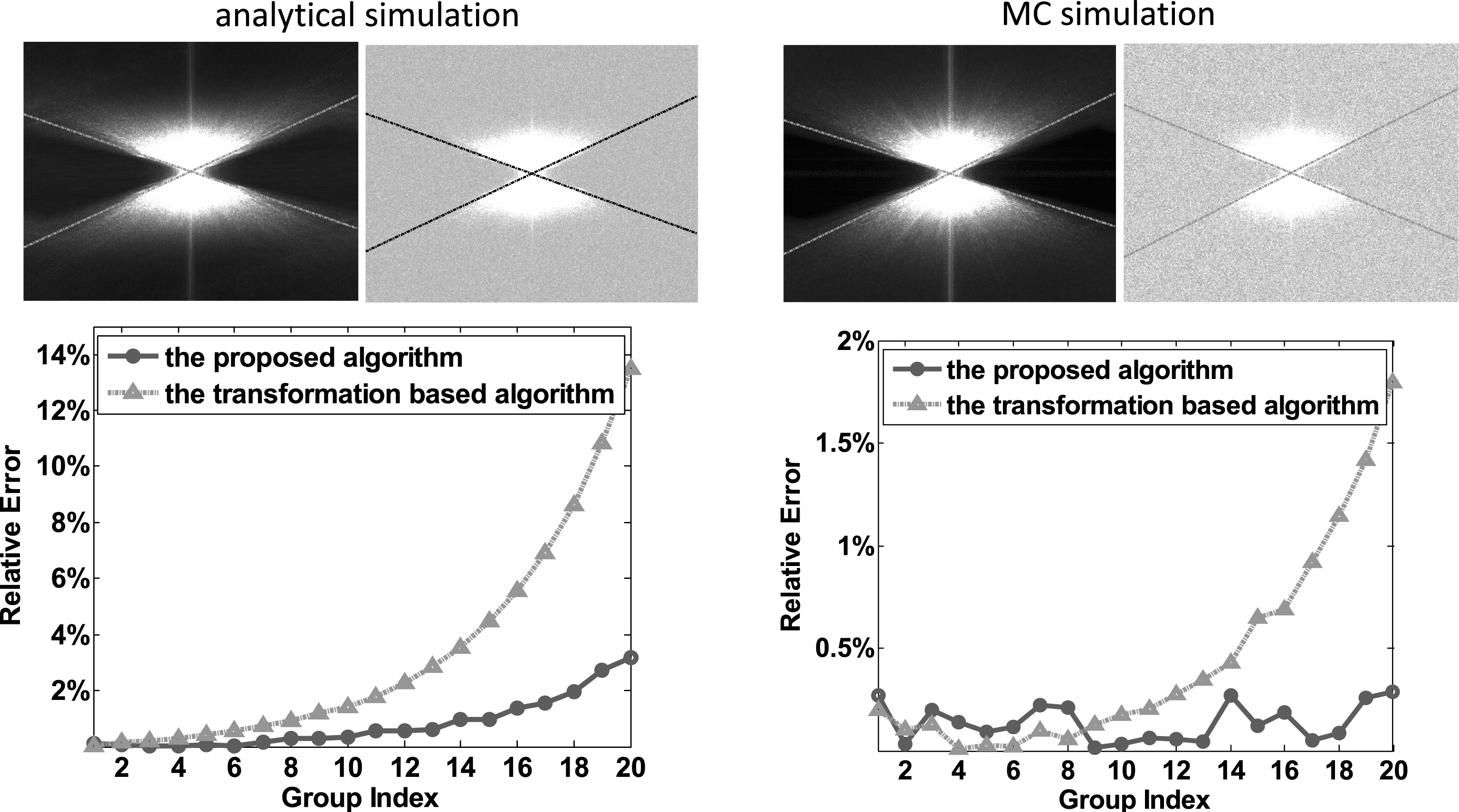
The first and the second columns correspond to the results of the analytical and the Monte Carlo simulations, respectively. In the first row of each column, left and right sub-figures are the maximum intensity projections along ξ direction of the 3D Fourier domain, corresponding to the noise-free and the noisy cone beam projections, respectively. In the first row, the dot dash lines are the detected boundaries with the line detector algorithm. The second row shows the comparisons of the relative errors between the proposed algorithm (circle marked solid line) and the transformation based algorithm (triangle marked dot dash line).

The second row of Fig. 3 plot the comparison curves of the relative errors calculated with the proposed algorithm and the transformation based algorithm. Quantitatively, with the proposed algorithm, the averaged relative errors across all the noise powers are 0.8% and 0.14%, corresponding to the analytical and the MC simulations, respectively. In addition, one also could observe that comparable results could be achieved for both algorithms when the noise power is high, however, as the noise power decreases (larger group index), the proposed algorithm could deliver more accurate results compared to the transformation based algorithm.

3.2 Simulation experiments under spotlight-mode

Figure 4 demonstrates the performance of the proposed algorithm when no sufficient information about the scanned object is available. It is shown that good noise level estimation performance still could be achieved, in terms of that the proposed algorithm is robust among different noise power settings, and be generally more accurate compared to the transformation based algorithm. Quantitatively, with the proposed algorithm, the averaged relative error across all the noise powers is 0.24%.

Fig.4

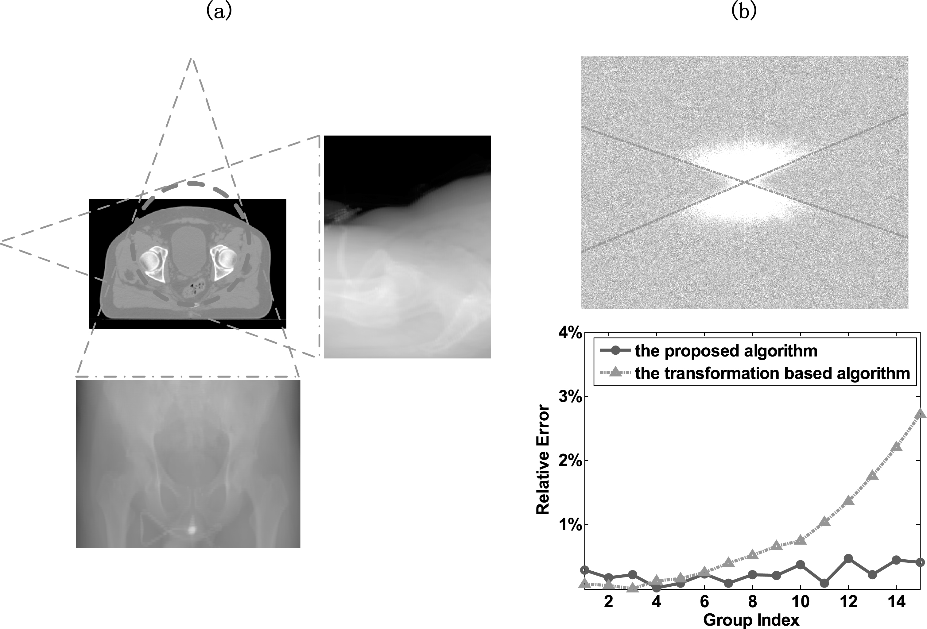
(a) Geometry illustration of the spotlight-mode, where no sufficient information about the object under scanned is available. The volume-of-interest inside the dash circle is centered on the prostate region. (b) simulation results. The first row is the maximum intensity projections along ξ direction of the 3D Fourier domain of the noisy cone beam projection data, where the dot dash lines are the detected boundaries with the line detector algorithm. The second row shows the comparison curves of the relative errors calculated with the proposed algorithm (circle marked solid line) and the transformation based algorithm (triangle marked dot dash line).

3.3 Comparison studies against the homogeneous area based algorithm

Figure 5 depicts the comparison results between the proposed algorithm and the homogeneous area based algorithm for all the above three experiments. Specifically, for the homogeneous area based algorithm, in the head-neck section based analytical and MC simulations, seven cuboids of dimension 5 × 5 ×5 centered in the points annotated by the numbers in Fig. 5(a) are chosen for the noise level estimation. Note that areas surrounding points 1∼4 could be regarded as flat, areas surrounding points 5 and 6 are relatively rugged, while the area surrounding point 7 belongs to the air-attenuated region. In the prostate section based spotlight-mode simulation, five cuboids with same dimensions are chosen, as shown in Fig. 5(d). In this case, areas surrounding points 3/4, 2/5 and 1 could be regarded as flat, relatively rugged and the air-attenuated regions, respectively. It is worth mentioning that the log scaled relative errors are used in Figs. 5(b), (c) and (e) due to the large disparities of the relative errors of the estimated noise levels associated with different areas, as the consequence of the non-uniform noise variance of cone beam projection data. It is shown that the relative errors of the homogeneous area based algorithm are systematically much higher than those with the proposed algorithm, and hence validates the superiority of the proposed algorithm. Besides, it is also observed that the curves corresponding to the air-attenuated regions keep constant, i.e., the relative errors of the estimated noise level based on the air-attenuated region are approximately 100%. The reason is that almost all of the noise in the air-attenuated region comes from the quantum noise associated with the blank-scan signal and the scatter signal, resulting a high signal-noise-ratio (SNR). Therefore, the estimated noise level based on the air-attenuated region would be very small, even to be zero which would result in a 100% relative error compared to the real noise level.

Fig.5

Comparison results between the proposed algorithm and the homogeneous area based algorithm. The first and the second rows correspond to the head-neck case and the prostate case, respectively. Sub-figures (a) and (d) are projection images in a certain view, where seven and five selected areas are annotated by the numbers, sub-figures (b), (c) and (d) are the log scaled relative errors of the estimated noise levels with both the homogeneous area based algorithm and the proposed algorithm, corresponding to the cases of analytical, MC and the spotlight-mode simulation experiments, respectively.

3.4 Real data experiments under short-scan/half-fan modes

Figure 6 demonstrates the results of the Catphan^® 600 phantom case. For the 13 groups of noisy cone beam projections, the estimated noise levels as well as the tube currents and the exposure times are tabulated in Table 3. Figure 6(b) plots the estimated noise levels and the mAs in a log-log scale. As the noise level should be inversely proportional to the mAs level, a straight line with a slope of -1 is expected in this plot. A linear fit indeed yields a slop of -1.0197, suggesting the efficacy of our noise level estimation algorithm.

Fig.6

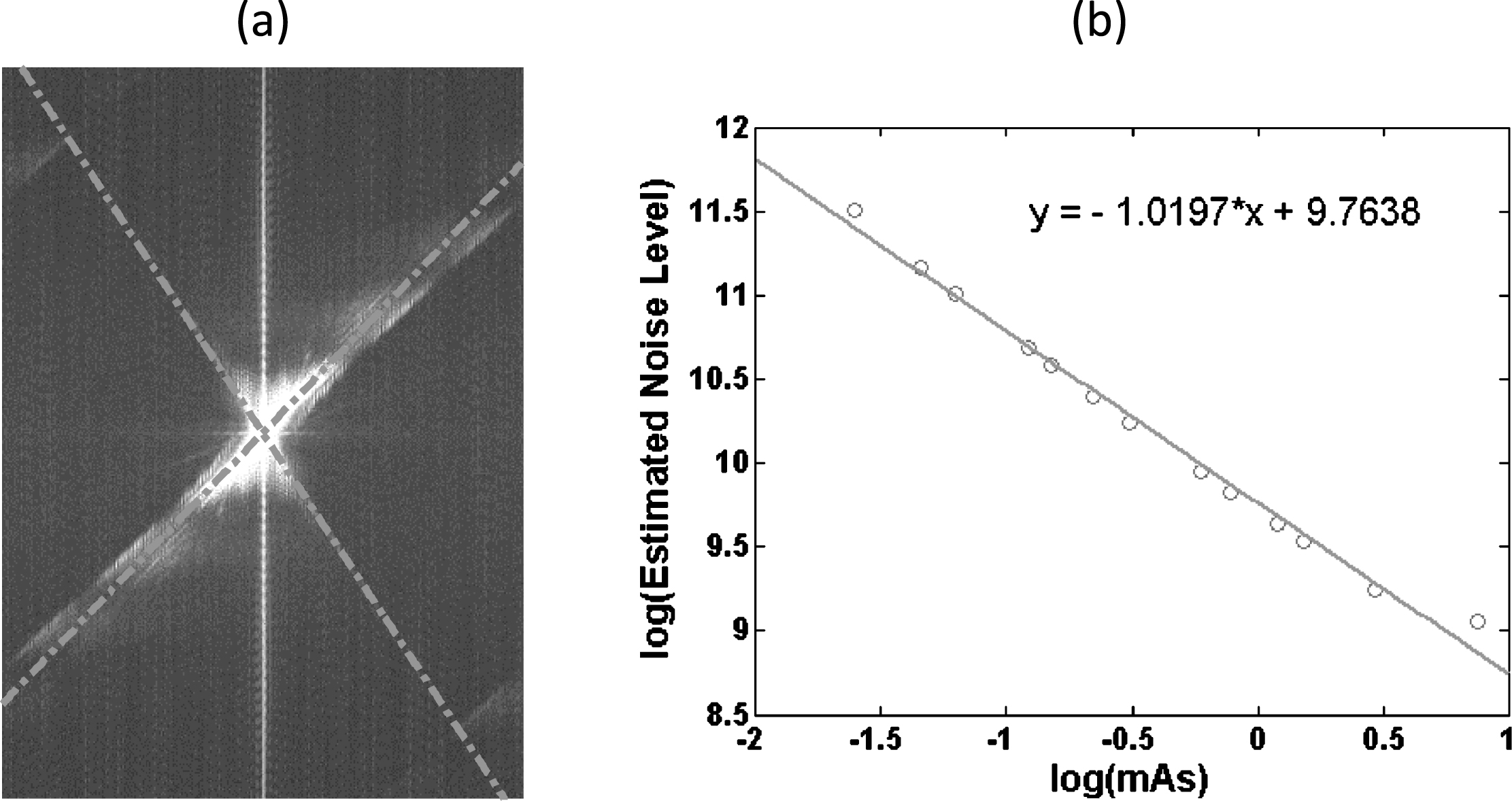
Result of the Catphan^® 600 phantom case. (a) shows the maximum intensity projection along ξ direction of the 3D Fourier domain of the real cone beam projection data scanned at 10 mA×20 ms exposure setting. The dot dash lines are the detected boundaries with the line detector algorithm. (b) log-log plot of the real exposure levels versus the estimated noise levels. The solid line shows the linear fit whose equation is presented in the upper-right corner.

Figure 7 demonstrates the noise level estimation results for the real data based on the anthropopathic physical phantom. It shows similarly promising results as those in Fig. 6, e.g., a linear equation with a slope of -1.0409 is obtained. More details about the tube currents, the exposure times as well as the estimated noise levels are summarized in Table 4.

Fig.7

The results for the pelvis section of the anthropopathic phantom case. The arrangements of the sub-figures are the same as those in Fig. 6.

3.5 Adaptive regularization parameter selection

Figure 8 demonstrates the reconstructed images of the Catphan^® 600 phantom. It is shown that as the dose level decreases, the FDK reconstructed images become noisier and noisier. In contrast, by using our adaptively selected regularization parameters, the regularized reconstructed images always exhibit high qualities in all dose levels. This result validates the practical utility of our estimated noise level. In details, for the 20 mA×20 ms and 40 mA×20 ms cases, as listed in Table 3, the estimated noise levels are 4.376 × 10⁴ and 2.088 × 10⁴, respectively. According to our selection strategy in Equation (20), λ is calculated to be 44.060 and 21.023, respectively.

Fig.8

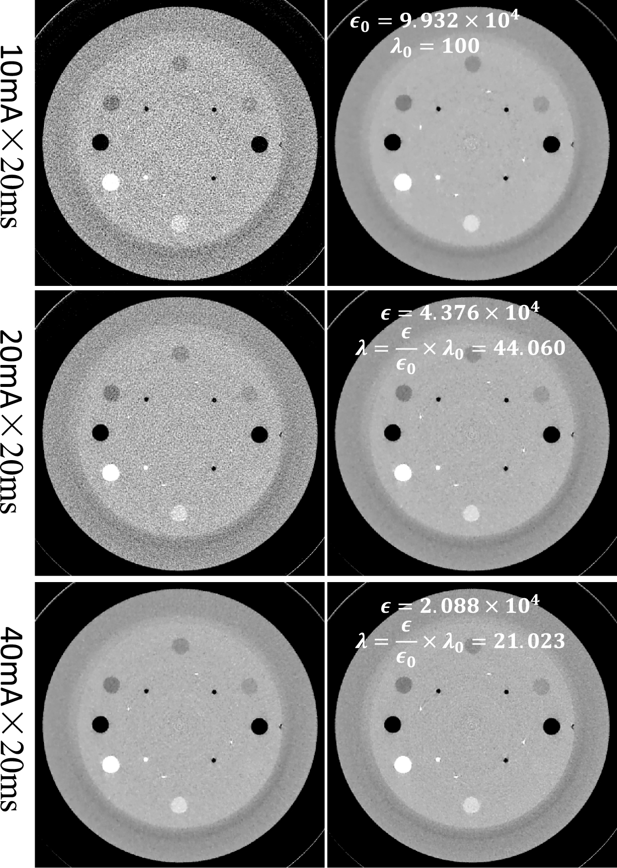
Reconstructed images of the Catphan^® 600 phantom. Images in the left and right columns correspond to the reconstructions with the FDK and the regularized iterative reconstruction algorithms, respectively. The first row is the reference case, the reference ɛ₀ and λ₀ are displayed in the right column. For the other two cases, the estimated ɛ and the selected λ are displayed in the corresponding regularized reconstructions. Display window: [0.1 0.3]cm^-1.

It is noted that Fig. 8 validates the effectiveness of the introduced parameter selection strategy based on the same phantom. It is meaningful to investigate its effectiveness among different cases. Figure 9 illustrates the reconstructed images of the HN patient and the anthropopathic physical phantom cases. For the HN patient case, using our proposed algorithm, the estimated noise level ɛ = 2.598 × 10⁵, the parameter λ is calculated to be 261.598. For the anthropopathic physical phantom case, ɛ = 9.071 × 10⁵, and λ = 913.310. Again, despite the large differences between the reference case and these two cases, the introduced parameter selection strategy still works well in terms of delivering promising image qualities with a balanced tradeoff between noise and resolution.

Fig.9

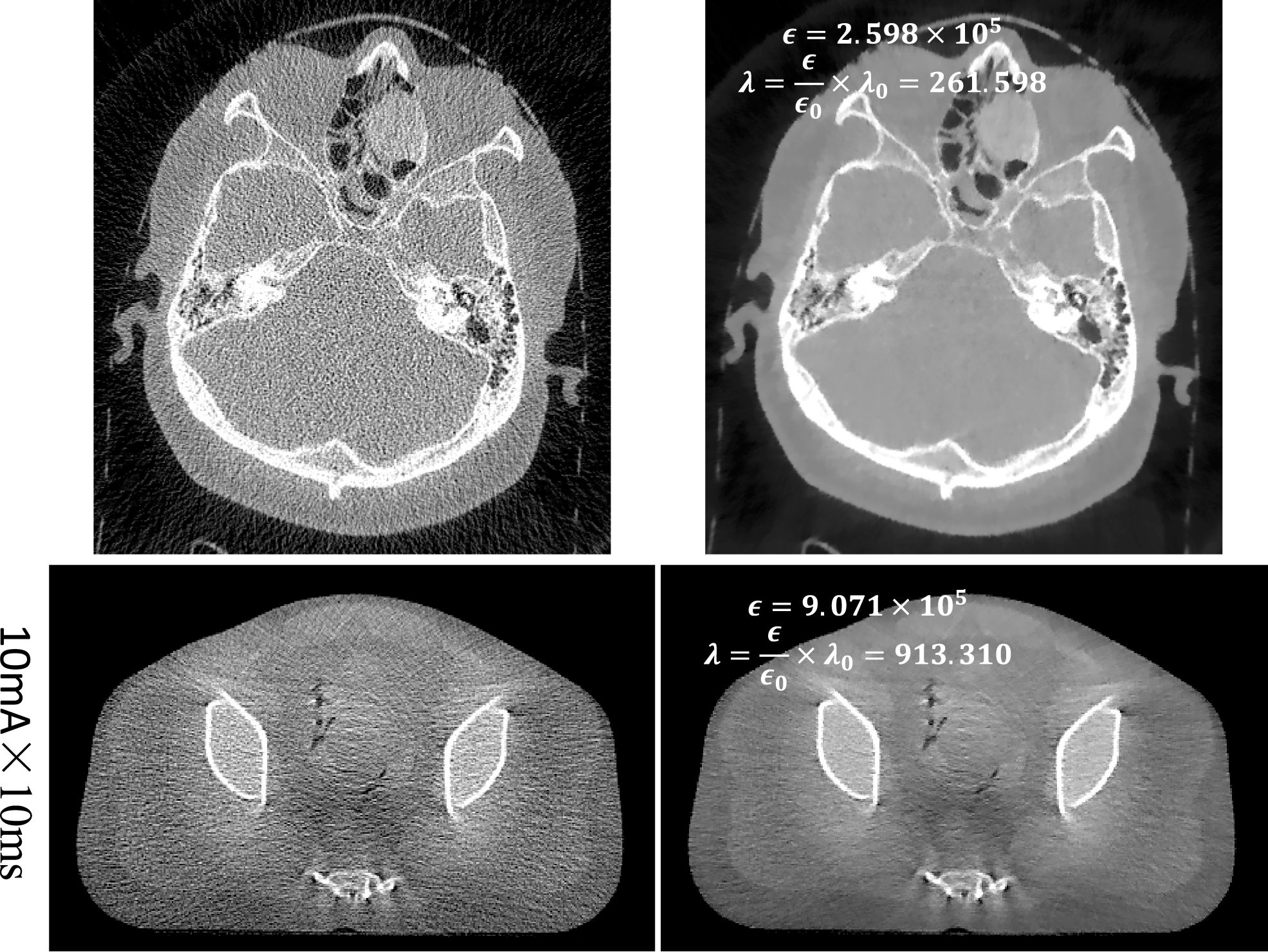
Reconstructed images of the HN patient case (row 1) and the anthropopathic physical phantom (row 2). Images in the left and right columns correspond to the reconstructions with the FDK and the regularized iterative reconstruction algorithms, respectively. The estimated ɛ and the selected λ are displayed in the corresponding regularized reconstructions. The display windows for the first and the second rows are [0 0.4]cm^-1 and [0.1 0.3]cm^-1, respectively.

Moreover, among all the studied cases, the minimum and the maximum λ are 21.023 and 913.310, respectively, having ∼50 times difference, suggesting the robustness of our strategy.

4 Discussions

In this work, we have demonstrated that there exists an approximately zero-energy double-wedge area in the 3D Fourier domain of cone beam projection data collected with a flat planar detector. By exploiting almost the same derivations as Section 2.2, similar data correlations are expected for the projection data from multiple detector computed tomography (MDCT) in the diagnostic imaging field. Moreover, as the data involved in this study are the line integrals, it also could be generalized to other imaging modalities, such as positron emission tomography (PET) and magnetic resonance imaging (MRI).

A potential application of our work is to facilitate the selection of the regularization parameter in a regularized iterative reconstruction scheme. In this work, we introduced a noise level driven adaptive regularization parameter selection strategy, as demonstrated in Section 2.5. Its performance has been validated under different dose levels and data cases, as presented in Section 3.5. This indicated that our selection strategy, i.e., Equation (20), also could be applied in other patient cases. Although the TV minimization based regularizer was employed in this work, it is believed that same selection strategy as Equation (20) could be also generalized to other regularizers such as the dictionary learning based sparse representation [7]. It is noted that this strategy is not intended to determine a final optimal λ which is always task-specific and also depends on the radiologists’ preference. Instead, our purpose is to demonstrate the practical utility of the estimated noise level with the proposed algorithm. A real clinic-accepted selection strategy still requires a further investigation which is our ongoing research.

In this work, we have conducted comparison studies between the proposed algorithm and the transformation based algorithm. And it turns out that the proposed algorithm could produce more accurate and robust noise level estimation results over the transformation based algorithm. It is worth mentioning that for the transformation based algorithm, a wise choice about the truncated high frequency is very important to enable an accurate noise level estimation, which is also case-by-case dependent. Moreover, the performance of the transformation based algorithm also depends on the image content and the noise power of the projection data. In other words, if the projection data contains substantial high frequency components, or the noise power is relatively low compared to the signal power, the performance of the transformation based algorithm would be hampered. For example, as observed from the simulation studies in Section 3, when the noise power was relatively low, the transformation based algorithm always performed worse compared to the proposed algorithm. In contrast, the accuracy and robustness of the proposed noise level estimation algorithm is theoretically ensured by our derived data correlation of cone beam projection data in Section 2.2. According to our derivation, there exists an approximately zero-energy double-wedge area in the 3D Fourier domain of the cone beam projection data. In other words, in this double-wedge area, the signal and the noise are well-decoupled regardless of the image content, the noise power, the scan geometry and etc. Moreover, the boundaries of the double-wedge area could be automatically detected by a Hough transform based line detector, which makes the proposed algorithm more practical. The experimental results also demonstrated that the proposed algorithm could consistently provide accurate and robust noise level estimations among different noise powers.

It must be pointed out that, in this work, the derived data correlation in the Fourier domain of cone beam projection data is based on the complete data sets, meaning that the theoretical integral intervals both for u and v should be from -∞ to +∞, and for β should be from -π to π in Equation (6). However, the practical integral interval for v could be relaxed to the lower and upper limits of the physical detector panel without impacts on our conclusion. This relaxed integration condition is ensured by the property of the delta function, i.e., the integration of f (x) δ (x - x₀) from a to b is f (x₀) as long as x₀ ∈ (a, b). Firstly, as shown in Equation (6), product of two delta functions is involved in the mathematical expression of the projection of some certain point, whose coordinate on the detector domain is (u₀ (β), v₀ (β)), i.e., p⁰ (u, v, β) = δ (u - u₀ (β)) δ (v - v₀ (β)). Secondly, projection of any point in the volume of interest would fall into the physical detector panel, in other words, it is valid that $v_{0} (β) \in (v_{l} o w e r, v_{u} p p e r) \subset (- \infty, + \infty)$ , where v_lower and v_upper denote the lower and upper limits of the physical detector panel. Combined with the above property of the delta function, these two facts confirm that the integration of v in (- ∞, + ∞) is exactly equal to that in (v_lower, v_upper), and hence, validates the relaxed integration condition. Undoubtedly, the relaxed integration conditions for u, v, β could be readily satisfied in most scenarios of MDCT. By contrast, in some CBCT applications such as the radiation therapy clinic, the short-scan mode (truncation in β direction) and the half-fan mode (truncation in u direction) are popular, and thus would violate the conditions. However, from our real data experiments in Section 3.4 that involves real data collected from both the short-scan and the half-fan modes, it was shown that the proposed algorithm still worked well without any additional data processing. Moreover, it is experimentally validated that even without sufficient information available about the object under scanned, the proposed algorithm still could estimate the noise level accurately, as shown in Section 3.2. More mathematical characterization is required for a better understanding about these results in the future.

5 Conclusions

There exists an approximately zero-energy double-wedge area in the 3D Fourier domain of cone beam projection data. The boundaries of the double-wedge area could be automatically detected with the Hough transform based line detector. The Fourier transformed noise is uniformly distributed, in terms of that for any point of the Fourier transformed noise, the expectation of the square of the amplitude is the same. Therefore, theoretically speaking, the signal and the noise are well-decoupled in the double-wedge area of the 3D Fourier domain. Based on the derived data correlation of cone beam projection data, guidelines regarding the estimation of the noise level of cone beam projection data are presented. Experimental results demonstrated that the proposed algorithm could estimate the noise level accurately and robustly. Additionally, to demonstrate the practical utility of our estimated noise level, a noise level driven adaptive regularization parameter selection strategy was introduced. Experiments demonstrated that across different dose levels and data cases, our strategy could always work well by delivering promising reconstructions with a balanced tradeoff between noise and resolution.

Footnotes

Acknowledgements

This work was supported in part by National Key Research and Development Program of China (No. 2016YFA0202003), in part by National Natural Science Foundation of China (No.61571359), in part by NIH (1R01CA154747-01, 1R21CA178787-01A1 and 1R21EB017978-01A1), in part by China Scholarship Council.

References

Van-Kranen

, Van-Beek Srasch

, Van-Herk

and Sonke

J.J.

, Setup uncertainties of anatomical sub-regions in head-and-neck cancer patients after offline cbct guidance, International Journal of Radiation Oncology Biology Physics 73(5) (2009), 1566–1573.

Kiljunen

, Kaasalainen

, Suomalainen

and Kortesniemi

, Dental cone beam ct: A review, Physica Medica 31(8) (2015), 844–860.

Wang

, Li

, Lu

and Liang

, Penalized weighted least-squares approach to sinogram noise reduction and image reconstruction for low-dose x-ray computed tomography, IEEE Transactions on Medical Imaging 25(10) (2006), 1272–1283.

, Li

, Chen

, Xing

, Jiang

and Liang

, Adaptive noise reduction toward low-dose computed tomography, Proc SPIE 5030 (2003), 759–766.

Sidky

E.Y.

and Pan

, Image reconstruction in circular conebeam computed tomography by constrained, total-variation minimization, Physics in Medicine and Biology 53(17) (2008), 4777–4807.

Niu

, Ye

, Fruhauf

, Petrongolo

and Zhu

, Accelerated barrier optimization compressed sensing (abocs) for ct reconstruction with improved convergence, Physics in Medicine and Biology 59(7) (2014), 1801–1814.

, Yu

, Mou

, Zhang

, Hsieh

and Wang

, Low-dose x-ray ct reconstruction via dictionary learning, IEEE Transactions on Medical Imaging 31(9) (2012), 1682–1697.

Chen

G.H.

, Tang

and Leng

, Prior image constrained compressed sensing (piccs): A method to accurately reconstruct dynamic ct images from highly undersampled projection data sets, Medical Physics 35(2) (2008), 660–663.

Jia

, Dong

, Lou

and Jiang

S.B.

, Gpu-based iterative cone-beam ct reconstruction using tight frame regularization, Physics in Medicine and Biology 56(13) (2011), 3787–3807.

10.

Ramani

, Liu

, Rosen

, Nielsen

and Fessler

J.A.

, Regularization parameter selection for nonlinear iterative image restoration and mri reconstruction using gcv and sure-based methods, IEEE Transactions on Image Processing 21(8) (2012), 3659–3672.

11.

Jin

, Zhao

and Zou

, Iterative parameter choice by discrepancy principle, Ima Journal of Numerical Analysis 32(4) (2012), 1714–1732.

12.

Bonesky

, Morozov’s discrepancy principle and tikhonov-type functionals, Inverse Problems 25(1) (2009), 015015.

13.

Ito

, Jin

and Takeuchi

, A regularization parameter for nonsmooth tikhonov regularization, SIAM Journal on Scientific Computing 33(3) (2011), 1415–1438.

14.

Abramov

S.K.

, Lukin

V.V.

, Vozel

, Chehdi

and Astola

J.T.

, Segmentation-based method for blind evaluation of noise variance in images, Journal of Applied Remote Sensing 2(1) (2008), 183–198.

15.

Salmeri

, Mencattini

, Ricci

and Salsano

, Noise estimation in digital images using fuzzy processing, Proc International Conference on Image Processing 1 (2001), 517–520.

16.

Corner

B.R.

, Narayanan

R.M.

and Reichenbach

S.E.

, Noise estimation in remote sensing imagery using data masking, International Journal of Remote Sensing 24(4) (2003), 689–702.

17.

Yang

S.M.

and Tai

S.C.

, Fast and reliable image-noise estimation using a hybrid approach, Journal of Electronic Imaging 19(19) (2010), 033007-033007-15.

18.

Donoho and David

, De-noising by soft-thresholding, IEEE Transactions on Information Theory 41(3) (1995), 613–627.

19.

Ponomarenko

N.N.

, Lukin

V.V.

, Zriakhov

M.S.

and Kaarna

, An automatic approach to lossy compression of aviris images, IEEE International Geoscience and Remote Sensing Symposium (2007), 472–475.

20.

Shin

D.H.

, Park

R.H.

, Yang

and Jung

J.H.

, Block-based noise estimation using adaptive gaussian filtering, IEEE Transactions on Consumer Electronics 51(1) (2005), 263–264.

21.

Wang

, Lu

, Liang

, Eremina

, Zhang

, Wang

, Chen

and Manzione

, An experimental study on the noise properties of xray ct sinogram data in radon space, Physics in Medicine and Biology 53(12) (2008), 3327–3341.

22.

Zhang

, Ouyang

, Ma

, Huang

, Chen

and Wang

, Noise correlation in cbct projection data and its application for noise reduction in low-dose cbct, Medical Physics 41(3) (2014), 59–65.

23.

Mazin

S.R.

and Pelc

N.J.

, Fourier properties of the fan-beam sinogram, Medical Physics 37(4) (2010), 1674–1680.

24.

Canny

J.F.

, Finding edges and lines in images, M.I.T. Artif. Intell. Lab., Cambridge, MA, TR-720, 1983.

25.

Deriche

, Using canny’s criteria to derive a recursively implemented optimal edge detector, International Journal of Computer Vision 1(1) (1987), 167–187.

26.

Nitin

and Clem

K.W.

, Line detection in images through regularized hough transform, IEEE Transactions on Image Processing 15(3) (2006), 582–591.

27.

Donoho

D.L.

, Compressed sensing, IEEE Transactions on Information Theory 52(4) (2006), 1289–1306.

28.

Siddon

R.L.

, Fast calculation of the exact radiological path for a three-dimensional ct array, Medical Physics 12(2) (1985), 252–255.

29.

Jia

, Yan

, Cervino

, Folkerts

and Jiang

S.B.

, A GPU tool for efficient, accurate, and realistic simulation of cone beam ct projections, Medical Physics 39(12) (2012), 7368–7378.

30.

Feldkamp

L.A.

, Davis

L.C.

and Kress

J.W.

, Practical cone-beam algorithm, Journal of the Optical Society of America A 1(6) (1984), 612–619.

Source -axis-distance L	100 cm
Axis-detector-distance D	50 cm
Detector size	0.0776 × 0.0776 cm²
Detector dimension	512 × 384
Number of projections over 2π	660
Phantom dimension	512 × 512 × 80
Voxel size	0.057 × 0.057 × 0.25 cm³

Data correlation based noise level estimation for cone beam projection data

Abstract

BACKGROUND:

OBJECTIVE:

METHODS:

RESULTS:

CONCLUSIONS:

Keywords

1 Introduction

2.1 Data correlation of CT sinogram in 2D Fourier domain

2.6.1 Simulation and comparison studies

Table 2 Cone beam geometry parameters for the real data Source -axis-distance L 100 cm Axis-detector-distance D 50 cm Detector size 0.0776 × 0.0776 cm2 Detector dimension 512 × 384 Number of projections over 200°(360°) 364(678)

3.1 Simulation experiments under ideal geometries

5 Conclusions

Footnotes

Acknowledgements

References

Table 2
Cone beam geometry parameters for the real data

Source -axis-distance L 100 cm

Axis-detector-distance D 50 cm

Detector size 0.0776 × 0.0776 cm²

Detector dimension 512 × 384

Number of projections over 200°(360°) 364(678)