Noise-robust Mojette reconstruction using sparse-view CT projections

Abstract

Sparse-view Computed Tomography (CT) has important significance in industrial inspection and medical diagnosis. Mojette transform is a kind of discrete Radon transform that can yield exact reconstructions instead of an approximate solution due to finite Radon sampling. However, the image is iteratively reconstructed pixel by pixel from corner to center, and the image error is proportional to the number of iterations. In this paper, we propose that there exist different sets of projection combinations to recover the original image within the close-to-minimal iterations. And a scheme is given to obtain multiple projection sets, each of which has the same number of minimum iterations and can recover a CT image with a similar level of small noise but different distributions. These images can be used further to restore the final CT image by counteracting noise with each other. The accuracy and validity of the proposed algorithm are verified by comparison with both other Mojette inversion algorithms and the classical SART algorithm.

Keywords

Radon transform Mojette transform close-to-minimal iterations counteracting-noise different sets of projection combinations

1. Introduction

Computed Tomography (CT) can effectively reconstruct the internal structure of the object, and it has been widely used in the field of industrial detection and medical diagnosis. Regarding the reconstruction technique, Radon transform is the theoretical basis of exact reconstruction in a continuous domain, whereas the detectors in an actual CT system are discrete and limited. Therefore, the image must be sampled to acquire discrete projection data, resulting in an approximate reconstruction error. Algebraic reconstruction techniques (ART) [1] and compressed sensing (CS)-based methods [2] are the main types of CT approximate reconstruction methods. When the projection data are insufficient, the image that is reconstructed by the algebraic reconstruction algorithm presents sharp artifacts and noise. As the advent of compressed sensing theory, Jørgensen et al. discussed the link between sparsity and sufficient sampling for CT reconstruction, so the Radon inversion reconstruction algorithms could realize a higher quality image from the insufficient projection data [3, 4]. Generally, image prior knowledge can be embedded in regularization to construct the CS reconstruction models, such as total variation (TV) regularization employing the image gradient sparsity [5, 6], higher-order derivative-based models [7, 8], dictionary-based sparse coding models [9, 10], wavelet and curvelet-based sparse models [11, 12], and deep residual learning for feature extraction [13, 14]. To date, many efforts have been devoted to mitigate the ill-posed problem that arises due to insufficient data, but the reconstruction error is still a problem when considering the presence of noise. To address the problems of reconstruction error and artifacts from a linear system with insufficient data based on the discrete Radon transform [15 –18], Mojette transform provides new ideas for exact sparse-view CT reconstruction [19]. It is inspiring to see that research efforts have been made to consider the transform from the acquired Radon projection to Mojette projection [20 –22].

Mojette transform is the theoretical basis of the exact CT reconstruction in the discrete domain. Mojette forward- and back-projection models are different from the traditional Radon-based reconstruction method. It establishes a one-to-one correspondence between the reconstructed pixel and the detector bin from the perspective of the discrete geometry. Since the discrete image domain, discrete projection domain and back-projection process are directly related to the establishment of a digital CT system, the Mojette inversion approach can reconstruct a discrete image from discrete sampling. A unique solution can thus be obtained for sparse-view CT reconstruction, which can fundamentally change the ill-posed problem according to the discrete geometry theory.

To address the problem of sparse-view CT reconstruction based on Mojette transform, Serviéres et al. [23] proposed the conjugate gradient method (CGM) on the discrete Mojette sampling geometry and implemented solutions of the inverse problem by minimizing the least square criterion. The conjugate gradient Mojette reconstruction estimated the image in each iteration. The high number of projections guarantees a lower number of iterations for image reconstruction, and an optimal solution is gained at a faster convergence rate. Normand et al. [24] used a geometrical approach to streamline the reconstruction process and defined different reconstruction paths from the starting point to destination. However, the method did not consider the projections that are gathered together to construct the optimal reconstruction path. Therefore, it cannot effectively reduce the noise propagation in the reconstruction process. Recur et al. [25] noted that the pixel values could be estimated by exploiting the Gaussian distribution of the corresponding bin set. The estimated pixels with a minimal error could be identified and reconstructed in each iteration. The smaller number of pixels reconstructed in each iteration leads to a higher number of iterations so that the overall error in the slice image is large in the case of fewer projections. Svalbe et al. [26] proposed a direct Mojette back-projection filtration algorithm, which generated results with the artifact such as the strong aliasing in the reconstructed image. When the number of projections is increased, the artifact at the center region is removed by using the FFT of the PSF, which is well conditioned. Kingston et al. [27] proposed a Fourier inversion reconstruction from Mojette projections that used exact frequency data re-sampling to make the slice data lie on a set of parallel lines in Fourier space. It required abundant slice data from the 1D projection DFT to tile the Fourier space so fewer artifacts would be introduced into the reconstructed results. Shekhar et al. [28] presented a robust method based on the classical Fourier inversion and generated compact sets of rational projections that are directly and exactly converted into Discrete Fourier Transform (DFT) space. However, a small redundancy in the Fourier space cannot spread out the noise and exponentially decreases the error in the reconstruction. In our previous work [29], the proposed priority-based Mojette inversion algorithm (PBI) takes projections in order of priority to minimize the noise multiplication factor for image reconstruction. The algorithm still cannot effectively suppress the error if there is a large amount of noise because Mojette transform is too sensitive to noise, especially in sparse-view CT reconstruction. Although some of above methods can acquire sufficient projection data to restore the original image, the results are not perfect, and the advantage of Mojette transform on the discrete geometry of the projection and reconstruction lattice is still not fully utilized in reconstruction schemes.

In this paper, we present a noise-robust Mojette reconstruction using multiple sparse-view images. The paper first extends the priority-based Mojette reconstruction approach by taking projections in order of priority [29], which has the advantage of yielding image reconstructions with minimal accumulation noise. Because more than one prioritized projection per iteration can be selected to implement the maximal number of pixels to minimize the accumulation noise, multiple projection sets are obtained by combining different selected projections. As a result, the paper obtains multiple projection sets to reconstruct multiple images for a 2D slice with a similar level of small noise but different distributions. Therefore, the proposed method can attenuate the noise effect by counteracting the noise among reconstructed CT images of the same slice and improve the performance without increasing the number of projections, which is more suitable for sparse-view CT reconstruction.

The paper is outlined as follows: Section 2 reviews Mojette transform and the priority-based Mojette inversion reconstruction (PBI). Section 3 defines PBI projection selection criterion by extending the PBI algorithm. Based on the proposed projection selection criterion, multiple projection sets can be obtained to reconstruct sparse-view CT images with a similar level of noise but different distributions. Then, the low-rank matrix restoration algorithm removes noise to find the most important elements and structures among these reconstructed CT images of the same slice. Section 4 shows the results of a comparison experiment in a noise environment and achieves better results than do several corner-based Mojette inversion algorithms.

2. Mojette transform and priority-based Mojette inversion reconstruction (PBI)

Mojette sampling using a Dirac pixel model is adapted to the discrete geometry of the reconstructed image f (k, l) where k stands for the columns and l for the rows, as shown in Fig. 1. Mojette projection angle, called simply a projection (p, q) in this paper, is denoted as θ = arctan(q/p) by the integer pair (p, q) corresponding to the number of pixel displacements in the horizontal and vertical directions. Note that p and q satisfy GCD (p, q) =1 and q is always positive, except for q = 0, p = 1. 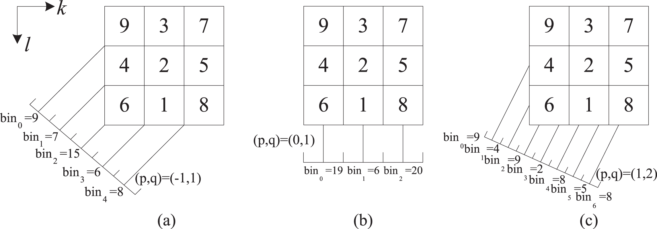The value M_p,q (b) is the sum of pixels centered on the parallel lines b = p · (l - 1) + q · (k - 1) for projection (p, q) and Dirac-Mojette definition is written as [30] $M_{p, q} (b) = \sum_{k = 1}^{P} \sum_{l = 1}^{Q} f (k, l) δ (b - q \cdot (k - 1) - p \cdot (l - 1))$ (1) where δ (·) is the discrete Kronecker function and the equi-spatial detector array includes b elements (called bins per projection). Based on discrete Mojette geometry, the total number of bins (rays) is computed by B = (P - 1) · |q| + (Q - 1) · p + 1 for a rectangular image P × Q, which depends on both the Mojette projection (p, q) and the image size P × Q. Obviously, for a N × N image array, the total number of rays (samples) in a projection set is denoted $N_{b i n s} = \sum_{i = 1}^{I} (N - 1) \cdot (| p_{i} | + q_{i}) + 1 = (N - 1) \cdot \sum_{i = 1}^{I} (| p_{i} | + q_{i}) + I$ . Projections (-1,1), (0,1), and (1,2), as acquired from the discrete geometry of a 3 × 3 image, are described as Fig. 1.

Fig.1

Results of Mojette sampling on a 3 × 3 image for projections (-1,1),(0,1),(1,2). (a) The value of bins in projection (-1,1) is 9, 7, 15, 6, 8. (b) The value of bins in projection (0,1) is 19, 6, 20. (c) The value of bins in projection (1,2) is 9, 4, 9, 2, 8, 5, 8.

Mojette back-projection can be accomplished from several different algorithms, and the classic corner-based Mojette inversion algorithm (CBI) is based on the mapping between the pixels and the projected bins. Katz theory indicates that the P × Q image can be exactly reconstructed from the minimal number of projections in a projection set (p_i, q_i) , i ∈ I, and it is formulated by [31] $\begin{matrix} \sum_{i = 1}^{I} p_{i} \geq p & o r & \sum_{i = 1}^{I} q_{i} \geq Q \end{matrix}$ (2) where I is the total number of projections. The condition can be extended to any convex region using mathematical morphology [20].

However, the traditional CBI that uses only the subtraction operation is very sensitive to noise. The image is iteratively reconstructed pixel by pixel from corner to center, and the reconstructed sequences of pixels are not fixed. In the extreme situation, only one single bin-pixel correspondence is found by the CBI in each iteration, which requires the maximum number of iterations to reconstruct an entire image. As a result, the noise propagates from the bins to the associated pixels at the maximum noise multiplication factor, and the CBI reconstruction contains the maximum noise accumulation. Considering the shortcomings of the CBI, the priority-based Mojette inversion method (PBI) improves its anti-noise performance. According to the reconstruction path determined by the prioritized projections, the PBI purposefully maps the maximal number of bins to the associated pixels in each iteration, which minimizes the number of iterations, resulting in minimal error in the reconstructed images. However, other than the corresponding bins of the determined reconstruction path, the bins do not make a significant contribution to the associated pixels, so the anti-noise performance of the PBI is limited in the case of large noise.

To enhance the anti-noise performance of the PBI in the case of large noise, a simple scheme is designed by considering various types of noise propagation along different reconstruction paths. From the CBI reconstruction process, the same image is known to have different reconstruction paths, and the different paths will cause different accumulation noise. Thus, the reconstructed images contain different noise distributions from different sets of finite noisy projections. Therefore, a simple scheme can overcome the disadvantage of the PBI by averaging the reconstructed images with different noise distributions for the same slice.

Fig.2

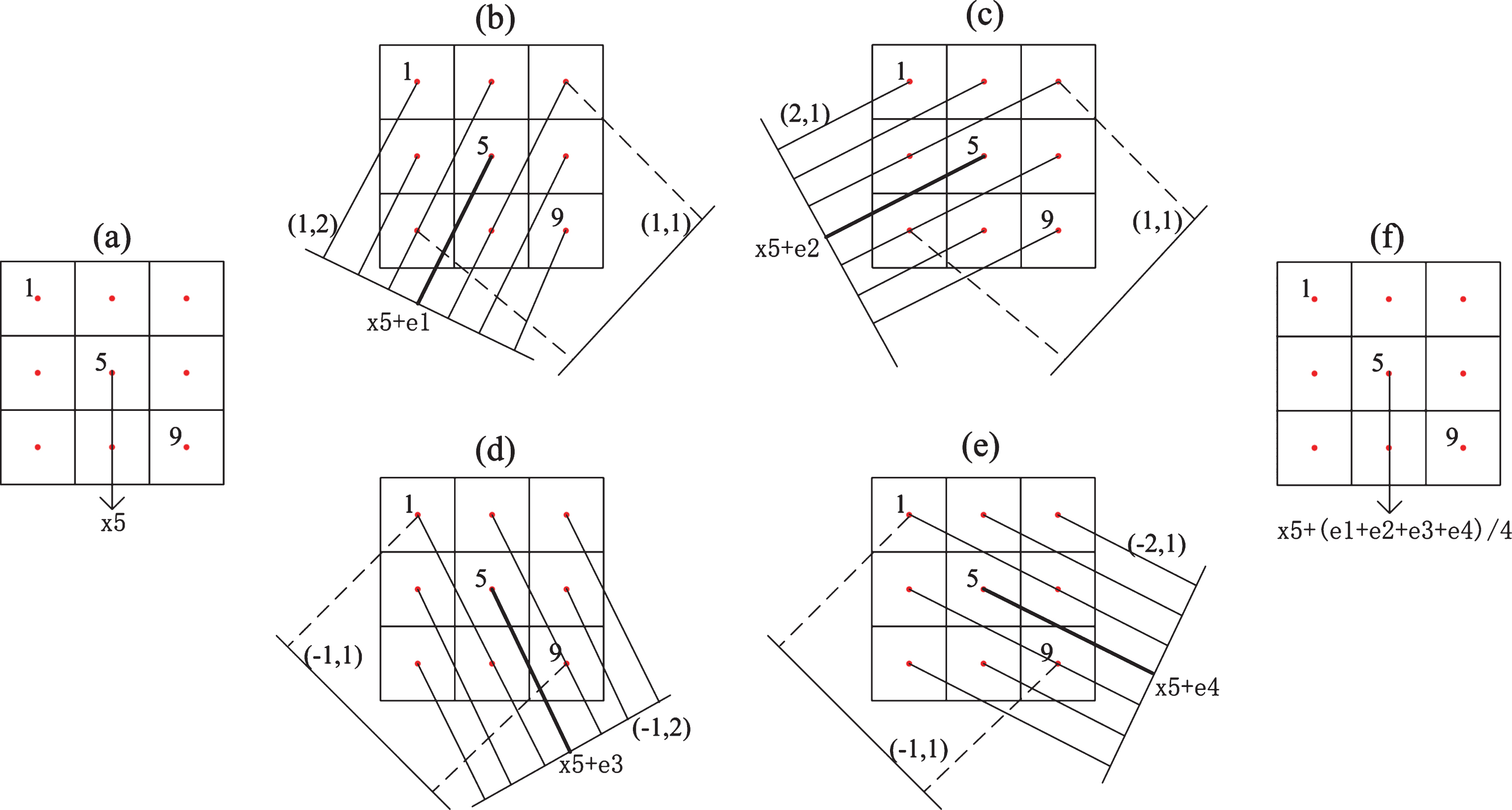
An example of one pixel reconstructed by averaging the pixel values at the same position of four reconstructed images. (a) is the original image, the values of pixel 5 in images (b)(c)(d)(e) are (x5 + e1), (x5 + e2), (x5 + e3), and (x5 + e4) with different random noise e1, e2, e3, and e4, respectively. (f) is reconstructed by averaging the pixel values in images (b)(c)(d)(e).

For example, Fig. 2 describes one pixel reconstructed by averaging the pixel values at the same position of four reconstructed images for a 2D slice. Images (b)(c)(d)(e) are reconstructed from four projection sets (1,2) (1,1), (2,1) (1,1), (-1,2) (-1,1), and (-2,1) (-1,1), where the values of pixel 5 are (x5 + e1), (x5 + e2), (x5 + e3), and (x5 + e4) with different random noise e1, e2, e3, and e4. Next, images (b)(c)(d)(e) are averaged to obtain a de-noised image, and the simple average improves the quality of the de-noised image, as shown in Fig. 2(f). Therefore, a scheme to average different reconstructions for the same slice can overcome the limitations of PBI caused only by a determined reconstruction path. Moreover, we can utilize a more complicated method such as low-rank matrix restoration algorithm to remove noise.

3. Strategies to improve the anti-noise ability of Mojette reconstruction

In this section, the paper first defines the PBI projection selection criterion and notes that more than one projection per iteration can be selected to implement the maximum number of pixels. This occurs because special Mojette discrete sampling leads to great changes in the projections with different size images and detector resolution. The optimal selection of projection combinations is imperative to minimize the accumulation noise on reconstructed images. Furthermore, different projection sets obtained by a combination of multiple selected projections are used to reconstruct multiple sparse-view CT images of the same slice with a similar level of noise but different noise distributions, and the slice can be restored by counteracting noise among these reconstructed CT images.

3.1. PBI projection selection criterion

The Mojette projection data in each bin are the sum of all pixels centered on the parallel line b = p_i · (l - 1) + q_i · (k - 1) for projection (p_i, q_i). Based on single bin-pixel correspondence, an image is fully reconstructed by mapping the bin values to the associated pixels in Mojette back-projection process. In the Mojette inversion reconstruction process, because of the noise that propagates from the bins to the associated pixels in each iteration, the noise multiplication factor increases as the number of iterations of image reconstruction increases. Thus, more noise accumulation leads to a poor quality of the reconstructed images. According to Mojette theory, the PBI maximizes the number of pixels in each iteration to speed up reconstruction; i.e., the image is reconstructed completely from the prioritized projections within the minimum number of iterations. Therefore, PBI projection selection criterion, simplified as the PBI criterion, was summarized to choose projections (p_i, q_i) with the maximum sum of p_i and q_i under the physical limit of detector resolution [29]. This criterion ensures the anti-noise performance of the PBI to recover images with the least amount of accumulation noise.

Fig.3

The number of pixels centered on the rays are respectively 6, 3, 2 in projections (1,1)(1,2)(1,3). (a). The ray intersects 6 pixels in projection (1,1). (b). The ray intersects 3 pixels in projection (1,2). (c). The ray intersects 2 pixels in projection (1,3).

Specifically, these selected projections (p_i, q_i) have the maximum number of rays (samples) B = (N - 1) · (|p_i| + q_i) +1 (see Section 2), and the smallest number of pixels is centered on each ray for the N × N image array. For example, Fig. 3 shows the interval of pixels and the number of pixels centered on the rays in projections (1,1), (1,2) and (1,3). Fig. 3 (a) shows the interval $\sqrt{p^{2} + q^{2}} = \sqrt{1^{2} + 1^{2}} = \sqrt{2}$ and the number of pixels $⌊ (\sqrt{2} \cdot N) / \sqrt{p^{2} + q^{2}} ⌋ = ⌊ \sqrt{2} \cdot N / \sqrt{1^{2} + 1^{2}} ⌋ = 6$ in projection (1,1). Similarly, there is the number of pixels $⌊ (\sqrt{2} \cdot N) / \sqrt{p^{2} + q^{2}} ⌋ = ⌊ \sqrt{2} \cdot N / \sqrt{1^{2} + 2^{2}} ⌋ = 3$ for the interval $\sqrt{p^{2} + q^{2}} = \sqrt{1^{2} + 2^{2}} = \sqrt{5}$ in projection (1,2) in Fig. 3 (b), there exists the number of pixels $⌊ (\sqrt{2} \cdot N) / \sqrt{p^{2} + q^{2}} ⌋ = ⌊ \sqrt{2} \cdot N / \sqrt{1^{2} + 3^{2}} ⌋ = 2$ for the interval $\sqrt{p^{2} + q^{2}} = \sqrt{1^{2} + 3^{2}} = \sqrt{10}$ in projection (1,3) in Fig. 3 (c). Therefore, when increasing the sum of p_i and q_i, the interval of pixels centered on the rays becomes large, and the number of pixels $⌊ (\sqrt{2} \cdot N) / \sqrt{p^{2} + q^{2}} ⌋$ decreases, where $\sqrt{2} \cdot N$ denotes the diagonal length across the N × N image.

Fig.4

Two pixels centered on the longest rays (e.g., the ray marked with the bold line) correspond to 4 iterations for 6 × 6 image reconstruction from projections (3,1) and (-3,1) with the large sum of p_i and q_i, where the results in each iteration are described in the top row. Moreover, the location of the reconstructed pixels in each iteration is marked with red dots in the bottom row. Pixels with red dots are obtained by the known pixels with black dots. Reconstruction paths from black pixel to the red pixel along bold lines describe the reconstructed sequences of pixels.

Fig.5

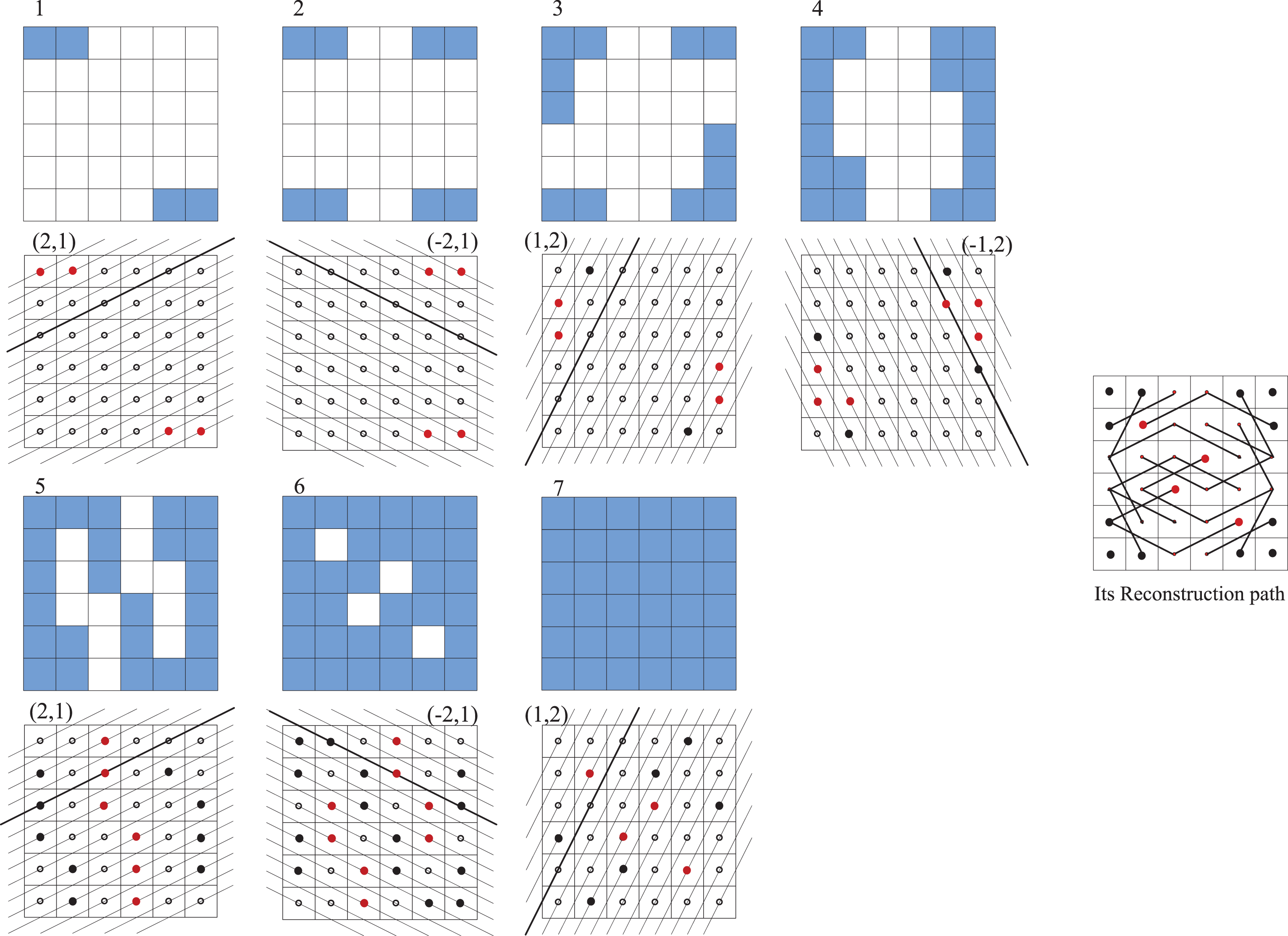
Three pixels centered on the longest rays (e.g., the ray marked with the bold line) correspond to 7 iterations for 6 × 6 image reconstruction from projections (2,1), (-2,1), (1,2) and (-1,2) with the small sum of p_i and q_i, where results in each iteration are described in the first and third rows, and the location of the reconstructed pixels in each iteration is marked with red dots in the second and fourth rows. Pixels with red dots are obtained by the known pixels with black dots. Reconstruction paths from the black to the red pixel along bold lines describe the reconstructed sequences of pixels.

Obviously, a small number of pixels leads to a small number of bin-pixel correspondences. When solving pixels from the periphery of the image to the center, the image is easily reconstructed in smaller iterations to yield an image with less accumulation noise. Briefly, different numbers of pixels correspond to different iterations for image reconstruction; two examples are shown in Figs. 4 and 5. Figure 4 shows two pixels centered on the longest rays (e.g., the ray marked with a bold line) corresponding to 4 iterations for the 6 × 6 image reconstruction from projections (3,1) and (-3,1) with the large sum of p_i and q_i, where the results in each iteration are described in the top row and the location of the reconstructed pixels in each iteration is marked with red dots in the bottom row. In the first iteration, six pixels are reconstructed because of the 3 × 2 single bin-pixel correspondence in corners of the discrete image. In the second iteration, pixels with black dots are known, so pixels with red dots are obtained by single bin-pixel correspondence. The reconstructed sequences of pixels are illustrated as reconstruction paths from black to red pixels along bold lines simultaneously. Similarly, Fig. 5 shows that three pixels being centered on the longest rays (e.g., the ray marked with a bold line) corresponds to 7 iterations for image reconstruction from projections (2,1), (-2,1), (1,2) and (-1,2) with the small sum of p_i and q_i. In the first iteration, there are four pixels to be reconstructed because of the 2 × 2 single bin-pixel correspondence in image corners, and so on. By comparison, projections (p_i, q_i) with the small sum of p_i and q_i correspond to more complex image reconstruction calculations because their reconstruction path is more complex than that of projections (p_i, q_i) with the large sum of p_i and q_i. Based on the above analysis, it is reasonable to select projections (p_i, q_i) with the maximum sum of p_i and q_i, which makes the small number of pixels centered on the longest projection rays through the discrete image.

Furthermore, we find that more than one projection in each iteration can implement the maximal number of pixels. There may be different sets of projection combinations that can be used to reconstruct the original image, and the reconstructed images show a similar level of noise but different distributions for the same slice. Given the scanning configuration that the reconstructed image size is 64 × 64, and the detector resolution is 1024; the Mojette projection (p_i, q_i) under this condition follows (64 - 1) · (p_i + q_i) +1 ≤ 1024, i.e.,p_i + q_i ≤ 16. According to the PBI criterion, PBI only selects projections with a sum of p_i and q_i equal to 16 to reconstruct the most number of pixels in each iteration; i.e., each selected projection has the same sum of p_i and q_i, which contains the same number of rays (samples) B = (N - 1) · (|p_i| + q_i) +1 for an N × N image array. Thus, different combinations of projections prioritized by the PBI can be utilized to restore the images within a few iterations.

For example, Table 1 shows that multiple projection sets contain the same number of projections and are comprised of projections (p_i, q_i) with the sum of p_i and q_i equal to 16; i.e., the total number of samples is the same in different projection sets. Their number of iterations is equal or close. The accumulation error in multiple reconstructed images for a 2D slice is almost the same but different in distribution.

The reconstructions from projection sets listed in Table 1 are shown in Fig. 6(a). We also illustrate image profiles along the 15th line of these images in Fig. 6 (b), so as to describe the differences among these reconstructed images in Fig. 6 (a). The error images between the original image and the reconstructed images are illustrated in Fig. 7(a). Similarly, Fig. 7 (b) shows image profiles along the 15th line of error images in Fig. 7 (a) to describe the differences among the error images. From the known error images, the noise distributions in the reconstructed images are quite different due to the difference in each reconstruction path from different sets of projections. Therefore, we can remove the noise by averaging all the reconstructed images to obtain the optimal solution for the original image. However, the reconstructed images from ten different sets of projections cannot effectively restore the original image. To achieve better image quality, many such projection sets should be selected.

Table 1

Different sets of projections and their corresponding iterations

Projection sets	Projections (p,q)	$\sum_{i = 1}^{I} (\| p_{i} \| + q_{i})$	Iterations
1st set	(11,5),(15,1),(-9,7),(-1,15),(9,7),(5,11),(-13,3),(-15,1),(-5,11),(1,15)	16*10	38
2nd set	(13,3),(15,1),(-9,7),(-1,15),(9,7),(5,11),(-13,3),(-15,1),(-5,11),(1,15)	16*10	39
3rd set	(11,5),(13,3),(-9,7),(-1,15),(9,7),(5,11),(-13,3),(-15,1),(-5,11),(1,15)	16*10	41
4th set	(11,5),(15,1),(13,3),(-1,15),(9,7),(5,11),(-13,3),(-15,1),(-5,11),(1,15)	16*10	46
5th set	(11,5),(15,1),(-9,7),(13,3),(9,7),(5,11),(-13,3),(-15,1),(-5,11),(1,15)	16*10	40
6th set	(11,5),(15,1),(-9,7),(-1,15),(13,3),(5,11),(-13,3),(-15,1),(-5,11),(1,15)	16*10	43
7th set	(11,5),(15,1),(-9,7),(-1,15),(9,7),(13,3),(-13,3),(-15,1),(-5,11),(1,15)	16*10	44
8th set	(11,5),(15,1),(-9,7),(-1,15),(9,7),(5,11),(13,3),(-15,1),(-5,11),(1,15)	16*10	42
9th set	(11,5),(15,1),(-9,7),(-1,15),(9,7),(5,11),(-13,3),(13,3),(-5,11),(1,15)	16*10	40
10th set	(11,5),(15,1),(-9,7),(-1,15),(9,7),(5,11),(-13,3),(-15,1),(13,3),(1,15)	16*10	44
11th set	(11,5),(15,1),(-9,7),(-1,15),(9,7),(5,11),(-13,3),(-15,1),(-5,11),(13,3)	16*10	38

Fig.6

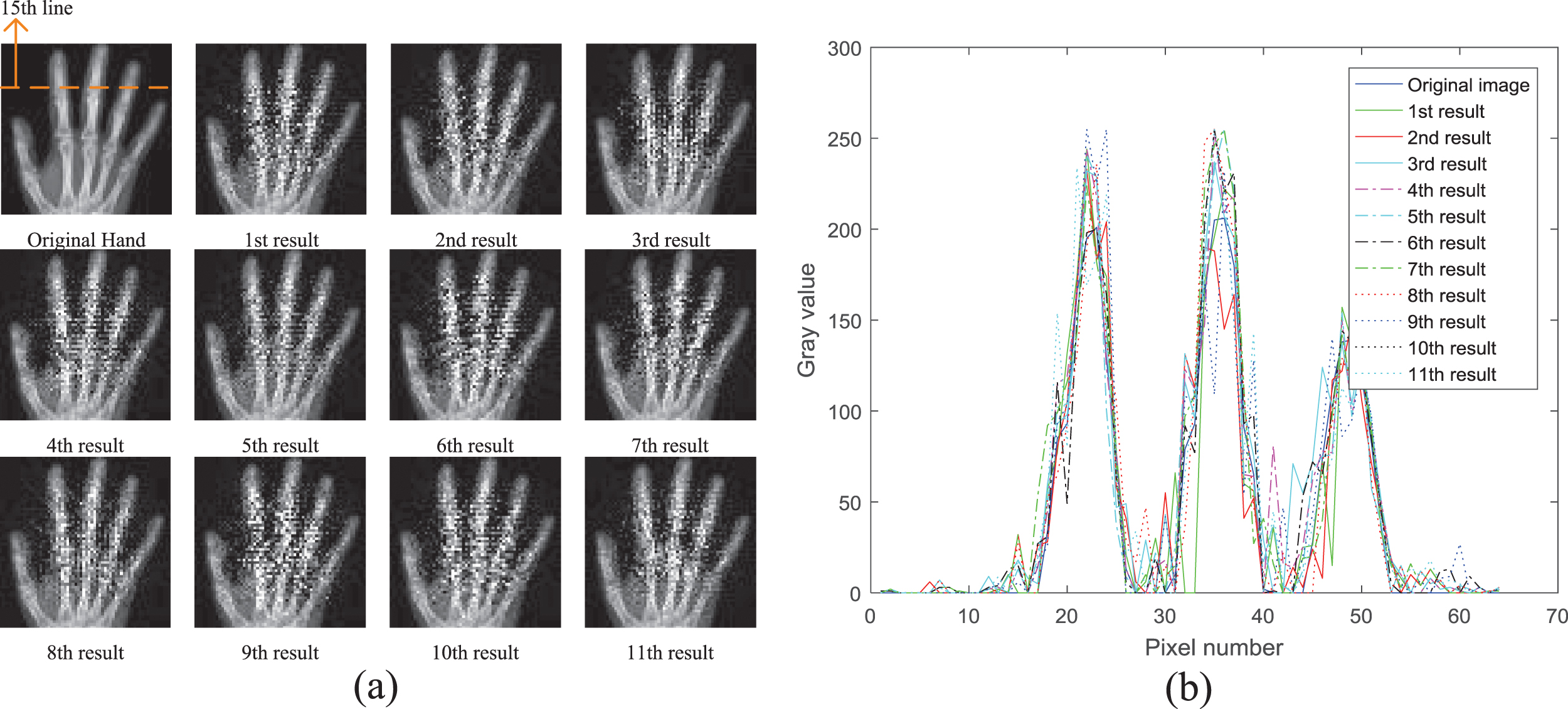
Differences among these reconstructed images. (a) The original image and its reconstructed images with different noise distributions from a set of ten projections in Table 1. (b) Image profiles along the 15th line of the images to describe the differences among the reconstructed images.

Fig.7

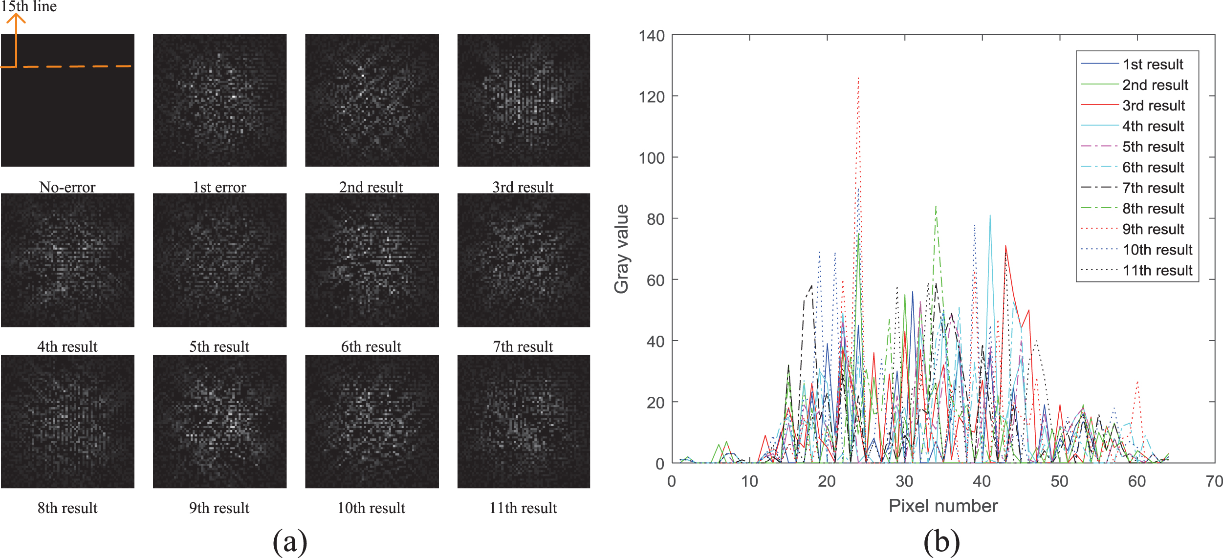
Differences among these error images. (a) The accumulation noises in the reconstructed images. Noise distributions in reconstructed images are quite distinct due to the difference in reconstruction paths from different projection sets. (b) Image profiles along the 15th line of the images in the horizontal directions to describe the differences among the error images.

It is known that the total number of rays (samples) in a projection set is denoted as $N_{b i n s} = \sum_{i = 1}^{I} (N - 1) \cdot (| p_{i} | + q_{i}) + 1 = \sum_{i = 1}^{I} B_{i}$ , the number of rays (samples) B = (N - 1) · (|p_i| + q_i) +1 per projection (p_i, q_i) is not greater than detector resolution, and the maximum sum of p_i and q_i is limited when both the size of the reconstructed image and the detector resolution are fixed. Based on the PBI projection selection criterion, the maximum sum of p_i and q_i directly determines the number of pixels to be reconstructed in each iteration. Thus, the stable value of iterations for image reconstruction remains at a numerical value due to the reconstructed number of pixels restricted by the maximum sum of p_i and q_i in each iteration. In summary, because of the Mojette sampling geometry, the maximum sum of p_i and q_i changes greatly for different image sizes and detector resolutions, the optimal selection of projection sets is imperative to minimize the accumulation noise.

3.2. The selection scheme of projection sets

From the description given in Section 3.1, the maximum sum of p_i and q_i in projection (p_i, q_i) makes great changes with different detector resolutions. As a result, the maximal number of pixels reconstructed in each iteration is quite different in various cases, leading to some changes in the stable value of iterations of image reconstruction. Thus, for a given-size image, the stable value of iterations for image reconstruction is limited by detector resolution, and the total number of data samples is determined by the sum of detector resolution B_i at different Mojette projections, denoted $N_{b i n s} = \sum_{i = 1}^{I} (N - 1) \cdot (| p_{i} | + q_{i}) + 1 = \sum_{i = 1}^{I} B_{i}$ , where I is the number of projections. In this section, the influence of detector resolution on the stable value of iterations is analyzed first, so the total number of data samples is adjusted to reconstruct different size images within the small stable value of iterations. Furthermore, a selection scheme to obtain different projection sets with equal number of data samples is proposed.

The influence of detector resolution on the stable value of iterations is shown in Fig. 8. The detector resolution and the stable value of iterations for image reconstruction are plotted as the horizontal and vertical axes, respectively. The red line illustrates that the stable value of iterations sharply drops from 449 to 1 as the detector resolution gradually increases from 512 to 4096 when reconstructing a 64 × 64 image. Similarly, there exists a decreasing trend for the 96 × 96 and 128 × 128 image reconstructions shown with blue and black lines, respectively. The diagram shows that the value of iterations decreases and trends to a smaller value for the reconstruction of a given-size image. A smaller number of iterations leads to less accumulation noise in the reconstructed images. Thus, 38 iterations, which is close to minimal, is considered a significant turning point of the curves because it ensures the reconstruction of images with little accumulation noise.

Fig.8

Influence of detector resolution on the stable value of iterations and the stable value of iterations for reconstructing a given-size image is followed by a significant downward trend with gradually increasing detector resolution.

Table 2 shows the sampling parameters affected by detector resolution for reconstructing images of different sizes, including the number of projections and iterations. With a number of data samples close to 2.50 × N², the PBI can reconstruct the images of different sizes within close-to-minimal 38 iterations. From the reconstruction parameters listed in Table 2, the maximum sum of p_i and q_i with the image size N is written as $\frac{Max (p_{i} + q_{i})}{N} = \frac{1}{4}$ , which is called the compact constraint for selecting projections with the nearly minimal 38 iterations. Geometrically, the maximum sum of p_i and q_i is one-fourth of the image size. Apparently, this results in a bigger ratio $\frac{Max (p_{i} + q_{i})}{N}$ , larger sum of p_i and q_i, and more data samples (rays) B = (N - 1) · (|p_i| + q_i) +1. It is well known that an image is easily reconstructed when the data samples increases.

Table 2

Reconstruction parameters affected by detector resolution

N × N	Resolution	Iterations	Number of projections	Max(p+q)	r	Data samples
64 × 64	1024	38	10	16	2.50	2.50 × N²
96 × 96	2304	42	10	24	2.50	2.50 × N²
128 × 128	4096	44	8	32	2.00	2.00 × N²

The quantitative analysis shows that when the relaxed constraints $\frac{Max (p_{i} + q_{i})}{N} \geq \frac{1}{4}$ are adopted to increase the data samples, there exists $⌊ (\sqrt{2} \cdot N) / \sqrt{{p_{i}}^{2} + {q_{i}}^{2}} ⌋ \leq 8$ after solving the Extremum Problems of binary quadratic equations for constant N. In other words, when $\frac{Max (p_{i} + q_{i})}{N} \geq \frac{1}{4}$ exists for an arbitrary image, the number of pixels centered on the projection rays keeps a reasonable proportion to the image size, and there are enough data samples in the projection set, so the number of pixels to be reconstructed in each iteration is nearly maximal and the number of iterations is close to the minimum. Obviously, the maximal number of pixels $⌊ (\sqrt{2} \cdot N) / \sqrt{{p_{i}}^{2} + {q_{i}}^{2}} ⌋$ centered on the longest projection rays through the discrete image, directly determine the iterations for image reconstruction, i.e., a smaller ratio $⌊ (\sqrt{2} \cdot N) / \sqrt{{p_{i}}^{2} + {q_{i}}^{2}} ⌋$ and more reconstructed pixels in each iteration (as described in Section 3.1).

To get the minimum number of iterations for an image reconstruction, constraints $\frac{Max (p_{i} + q_{i})}{N} \geq \frac{1}{4}$ or $⌊ (\sqrt{2} \cdot N) / \sqrt{{p_{i}}^{2} + {q_{i}}^{2}} ⌋ \leq 8$ should be satisfied. Equivalently, if $\frac{Max (p_{i} + q_{i})}{N} \geq \frac{1}{4}$ holds, when the total number of samples in the selected projection sets reaches 2.5 × N², this value is sufficient to achieve image reconstructions with the minimal accumulation noise. Based on the above qualitative analysis, the 64 × 64, 96 × 96 and 128 × 128 images can be reconstructed from 2.5 × N² samples within the close-to-minimal 38 iterations, as shown in Table 2.

From the qualitative analysis given above, a new selection scheme for a set of projections is based on both the compact constraint $\frac{Max (p_{i} + q_{i})}{N} \geq \frac{1}{4}$ and 2.5 × N² reasonable samples. Multiple projection sets can reconstruct multiple images for a 2D slice with a similar level of accumulation noise, by which the stable value of iterations to reconstruct the image remains low. These reconstructed images have different noise distributions due to their different reconstruction paths, and they can be used with each other to counteract the noise and thereby obtain a better image.

3.3. Noise-robust Mojette reconstruction

In Section 3.2, the proposed selection scheme of projection sets can yield multiple sets of projections to reconstruct multiple CT images for the same slice in close-to-minimal iterations. Thus, multiple reconstruction images for the same slice are obtained with a similar level of small accumulation noise. To make rational use of multiple reconstructed images to remove noise, this paper adopts the theory of low-rank recovery to restore the original image. It is acknowledged that low-rank theory can effectively remove noise and redundancy to find the most important elements and structures in data space. In this paper, each reconstructed image with small accumulation noise can be considered a column of the low-rank matrix. The columns in the observation matrix are linearly dependent and noise distribution in the matrix columns is sparse. Therefore, low-rank theory can achieve the optimal estimation of the original image A from the corrupted observations D = A + E, where some entries of the additive errors E may be arbitrarily large [32, 33]. Here, the Inexact Augmented Lagrange Multiplier Method (IALM), a typical solution of Robust principal component analysis (RPCA) problem, is utilized to estimate the optimal solution for the original image [34, 35]. Therefore, noise-robust Mojette reconstruction, also called the PBI-IALM reconstruction, is summarized in the following procedure:

(1) Obtaining multiple projection sets: Given a N × N image and detector resolution B, projections (p_i, q_i) must satisfy the acquisition requirement for Equation (3), $(N - 1) | p_{i} | + (N - 1) | q_{i} | + 1 \leq B$ (3) Based on the proposed selection method of projection sets, each projection with the maximum sum of p_i and q_i is selected in each iteration until the total number of samples contained in the selected projections reaches 2.5 × N² for N × N image reconstruction. For example, there are 16 total projections with a maximum sum of p_i and q_i for 64 × 64 image reconstruction, and any 10 projections can be used to reconstruct images because there are 2.5 × N² data samples in each set of projections, as shown in Table 1. Therefore, there exist $C_{16}^{10}$ different sets of projection combinations to recover the original image.

(2) Reconstructed images from multiple projection sets: Multiple projection sets are used to reconstruct the images fⁿ (k, l) by using the PBI. Thus, different reconstructions for a 2D slice are obtained and contain similar levels of noise but different noise distributions.

(3) Each of the multiple reconstructed images is considered a column of the corrupted observation matrix: Wright et al. showed that as long as the error matrix E is sufficiently sparse, one can recover a precise low-rank matrix A from the corrupted observations D=A+E by solving the RPCA problem: $min_{A, E} ∥ A ∥_{*} + λ \cdot ∥ E ∥_{1}, s . t ., D = A + E$ (4) For the RPCA problem (4), we apply the inexact augmented Lagrange multiplier method (IALM) by identifying $X = (A, E), f (X) = ∥ A ∥_{*} + λ \cdot ∥ E ∥_{1}, and h (X) = D - A - E$ (5) The solving procedure for the IALM algorithm is described in a previous paper [35]. Each reconstructed image fⁿ (k, l) in step 2 is considered a column of observation matrix {D = (fⁿ (k, l))} ∈ R^(P×Q)×n, which is corrupted by the accumulation noise E. Meanwhile, a positive weighting λ is used to constrain the optimization problem.

(4) The optimal estimate of the original image: Finally, a low-rank matrix A can be recovered by using the IALM algorithm, and any column of matrix A is the optimal estimate of the original image.

In conclusion, this proposed selection scheme of projection sets can be applied to select many projection sets and obtain different reconstructions for a 2D slice using the PBI. The IALM algorithm can be used to remove the accumulation noise. A greater number of reconstructed images for a 2D slice and a higher quality result from the use of IALM.

4. Experiments and results

To verify the performance of the proposed algorithm, experiments are designed in this section. The accuracy and validity of the algorithm are verified by comparison with both other Mojette inversion algorithms and the classical SART algorithm.

We only perform mathematical simulations to verify our method in experiments. To verify the anti-noise performance of the noise-robust Mojette reconstruction from sparse-view CT images, the number of sparse-view CT images is gradually increased by increasing the number of projections according to the selection scheme of projection sets. To further demonstrate the validity and accuracy of the proposed PBI-IALM algorithm, the PBI-IALM is compared with several corner-based Mojette inversion algorithms and the classical SART algorithm.

4.1 Noise-robust Mojette reconstruction

Based on discrete Mojette geometry, the acquisition data are collected along the parallel rays at projection angles to achieve exact and noise-free projection data [36]. The projection angles are non-uniformly distributed over [0, π]. To demonstrate the validity and accuracy of the proposed method in reducing the noise effect, a random uniform noise in the interval [-0.5 % M_max, 0.5 % M_max] is introduced into the Mojette projection data, where M_max = max{ M_p,q (b) , (b, p, q) ∈ M } [25].

According to the proposed selection scheme of projection sets, the method to select Mojette projection sets in this experiment is first described as follows. From Section 3, we know that the sampling data should satisfy both the PBI compact constraint $\frac{Max (p_{i} + q_{i})}{N} \geq \frac{1}{4}$ and the acquisition requirement (N - 1) · (|p_i| + q_i) +1 ≤ B. For a 1024 equi-spatial detector array, if the image size is 64 × 64, the sum of p_i and q_i is not greater than 16, i.e., (|p_i| + q_i) ≤16. By calculation, the sum of 16 projections (p_i, q_i) reaches the maximum value; the projections are (15,1), (13,3), (11,5), (9,7), (7,9), (5,11), (3,13), (1,15), (-15,1), (-13,3), (-11,5), (-9,7), (-7,9), (-5,11), (-3,13) and (-1,15). Any of the 16 projections can be selected in each iteration until the data samples in all the selected projections reach 2.5 × 64² for a 64 × 64 image reconstruction. Thus, any set of ten projection combinations with the sum of p_i and q_i equal to 16 in each iteration can be selected to fully reconstruct an image. In addition, different sets with ten projections are obtained because the constraints $\frac{Max (p_{i} + q_{i})}{N} \geq \frac{1}{4}$ and the requirement of 2.5 × N² total samples are satisfied.

Specifically speaking, when we arbitrarily choose 15 of the above 16 projections, then $C_{15}^{10} = 3003$ projection combinations are obtained. Similarly, choosing 14 of the above 16 projections is corresponding to $C_{14}^{10} = 1001$ sets of projections, and so on. To verify the influence of the number of sets of projections on the reconstruction quality, we used some of the projections from $C_{10}^{10} = 1$ , $C_{13}^{10} = 286$ , $C_{14}^{10} = 1001$ and $C_{15}^{10} = 3003$ , e.g., extracting 1, 165, 735, and 1775 sets of projections, respectively. Thus, without greatly increasing the number of projections, multiple projection sets were obtained to reconstruct multiple CT images of the same slice with similar levels of small noise but with different distributions.

Fig. 9 shows the results restored from 1, 165, 735, and 1775 projection sets by the PBI-IALM algorithm in the [-0.5 % M_max, 0.5 % M_max] noise environment, where (a)(f)(k)(p) are the original images. The results (b)(g)(l)(q) are reconstructed from one projection set, in which the center regions are destroyed by the accumulation noise. Because only one image is considered the corrupted observation, the PBI-IALM is nearly ineffective in removing the accumulation noise in center regions. By using 165 reconstructed images as corrupted observations to estimate the original images, the PBI-IALM algorithm gives an optimization solution (c)(h)(m)(r) by solving the convex optimization problem (4) in Section 3.3. The comparative results (b)(g)(l)(q) show that the noise in results (c)(h)(m)(r) were amazingly removed by the PBI-IALM algorithm. More useful information is applied to solve the RPCA problem as a result of using more sparse-view CT images for the 2D slice. Thus, the results (d)(i)(n)(s) were further improved as the number of reconstructed images became 735. Similarly, utilizing 1775 reconstructed images, the results (e)(j)(o)(t) became clearer and approached the original images. A comparison of the last two columns showed that the images were nearly the same. Therefore, 735 reconstructed images were enough to counteract noise; i.e., an increase of only 4 on the basis of 10 projections was sufficient to obtain enough sets of projection combinations, from which a final CT image was restored by removing the noise among their reconstructed CT images of the same slice.

Fig.9

The reconstruction results from 1, 165, 735 and 1775 sets of projections by using the PBI-IALM algorithm in [-0.5 % M_max, 0.5 % M_max] noise environment.

Image quality metrics between the reconstructed images and the original images are computed by the Structural SIMilarity (SSIM) criterion [37]. The closer the SSIM value is to 1, the better the reconstruction quality is. Moreover, the Peak Signal to Noise Ratio (PSNR) is used as an objective criterion for denoising. Fig. 10 shows the error images between sub-figures (e)(j)(o)(t) in Fig. 9 and their original images.

The experimental results demonstrate that the PBI-IALM algorithm can effectively remove large accumulation noise in the center region. To further demonstrate the anti-noise performance of the proposed PBI-IALM algorithm, the PBI-IALM is compared with several corner-based Mojette inversion algorithms, including the CBI, NR-CBI and PBI, in the following section.

Fig. 10

The accumulation noise on different pixels is reflected through 3D surface graph of the error images (a)(b)(c)(d) between sub-figures (e)(j)(o)(t) in Fig. 9 and its original images (a)(f)(k)(p).

4.2 Comparison experiments with similar corner-based Mojette inversion algorithms

Comparison experiments with similar corner-based Mojette inversion algorithms are done to demonstrate the performance of the proposed robust algorithm against the accumulation noise. To ensure a comparison in the same noise environment given in [25], 2048 equi-spatial detector array is set for the 64 × 64 image reconstruction in a [-2.5 % M_max, 2.5 % M_max] noise environment. Moreover, noise robustness is also measured with signal to noise ratio (SNR). In the experiments, we extract 16 projections with the maximal sum of p_i and q_i from 15-order Farey series [38], from which the PBI, CBI and PBI-IALM are used to reconstruct the images. The NR-CBI reconstructs the images from 128 projections from the 10-order Farey series given in [25]. Notably, the 2048 detector resolution is sufficient for the number of the projection rays (samples) at all projections from both the 10-order and 15-order Farey series. According to the Mojette property, the total number of data samples included in the 16 projections with the maximal sum of p_i and q_i is far less than that in the 10-order Farey series, and the same situation occurs for the number of projections.

Fig. 11 shows the comparison results of PBI, CBI, NR-CBI and PBI-IALM, where (a)(f) are the original images. The results (b)(g) are reconstructed from 16 projections by the CBI, results (c)(h) from 16 projections by the PBI, results (d)(i) from 128 projections from 10-order Farey series by the NR-CBI in [25] and results (e)(j) from 16 projections by the PBI-IALM, as shown in Table 3. The experiments indicate that CBI and PBI fail to get the results shown as figures (b)(g)(c)(h) in a high noise environment. Compared with the results (d)(i) of NR-CBI, the results (e)(j) obtained by the proposed PBI-IALM algorithm were quite good. In conclusion, the proposed algorithm has obvious advantages in resisting noise interference in a large noise environment.

Fig.11

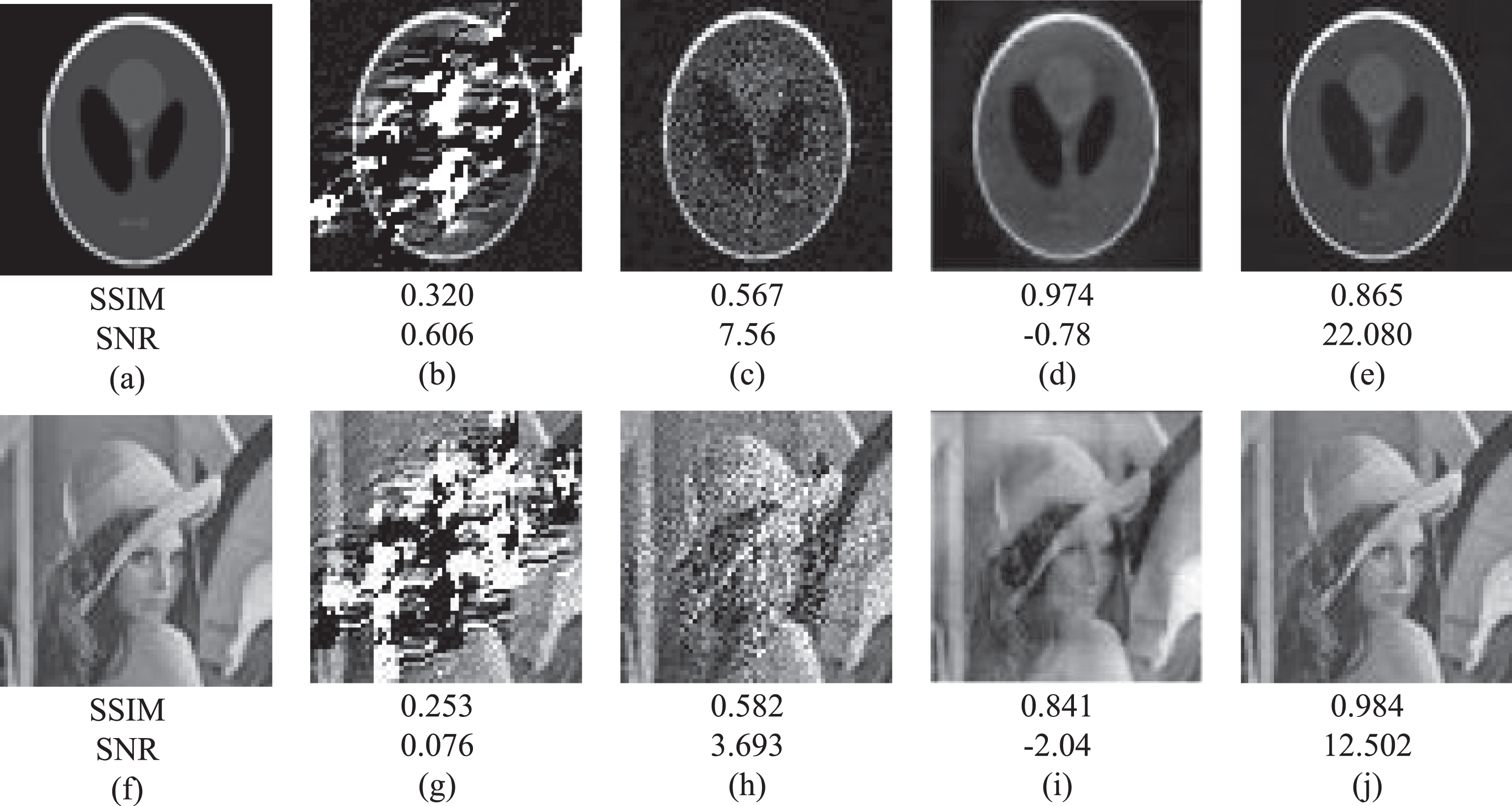
Comparison experiments with similar corner-based Mojette inversion algorithms in [-2.5 % M_max, 2.5 % M_max] noise environment given in [25]. (a)(f) are the original images, results (b)(g) are reconstructed from 16 projections by the CBI, results (c)(h) from 16 projections by the PBI, results (d)(i) from 128 projections by the NR-CBI in [25] and results (e)(j) from 16 projections by the PBI-IALM.

Table 3

Comparison with similar corner-based Mojette inversion algorithms

Algorithms	CBI	PBI	NR-CBI	PBI-IALM
Results	(b)(g)	(c)(h)	(d)(i)	(e)(j)
Number of projections	16	16	128	16

Fig. 12 shows comparable results for using the PBI-IALM and the SART in a [-2.5 % M_max, 2.5 % M_max] noise environment. As shown in Fig. 12, (a)(d) are the original images, results (b)(e) are obtained by the PBI-IALM from 16 projections with the maximal sum of p_i and q_i from the 15-order Farey series, and results (c)(f) are obtained by the SART from 16 projections uniformly distributed between 0 and π. Comparisons between the SART and the PBI-IALM are depicted in detail in the following section.

Fig.12

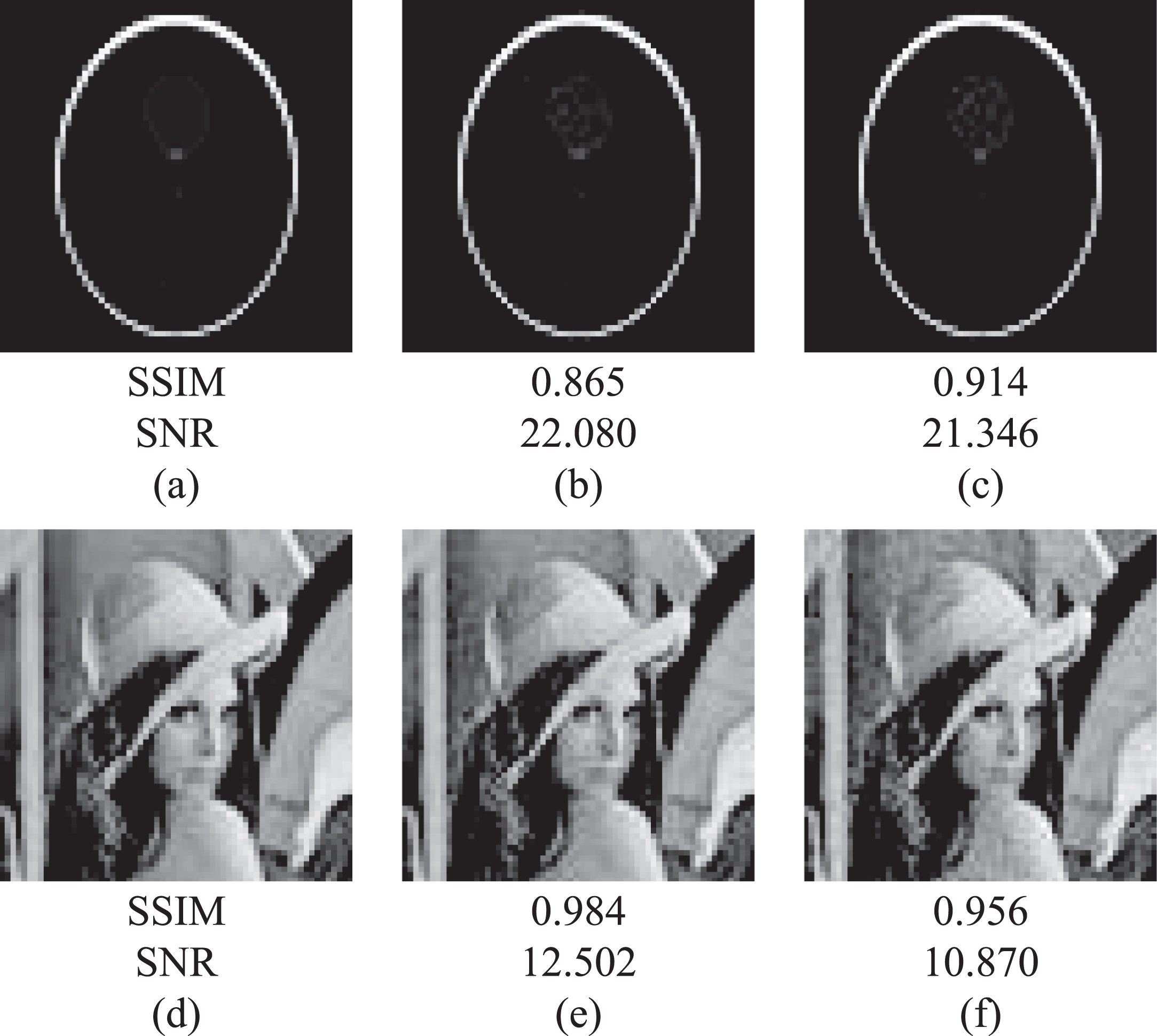
Comparable results by the PBI-IALM and SART in [-2.5 % M_max, 2.5 % M_max] noise environment. (a)(d) are the original images, results (b)(e) are obtained by the PBI-IALM from 16 projections, results (c)(f) are obtained by the SART from 16 projections.

4.3 Comparison experiments with the traditional SART

The paper proposes a new reconstruction algorithm based on Mojette transform, which is different from the traditional Radon-based SART algorithm. Comparison experiments with the traditional SART are done and shown in Fig. 13, where (a)(b)(c)(d)(e)(f) are the original images. From the comparison results shown in Fig. 13, the results (g)(h)(i)(j)(k)(l) by PBI-IALM are generally comparable with the results (m)(n)(o)(p)(q)(r) by the SART from the same number of projections in the [-0.5 % M_max, 0.5 % M_max] noise environment, where the projection error with ±0.5% is not too small for a x-ray image receptor. Specifically, the PBI-IALM algorithm can yield better results than those obtained by the SART in the peripheral regions of images, but the results are slightly worse than those of the SART in the center of the images. For instance, Fig. 14 shows image profiles along the 7th line of the images (i.e., the periphery of the images) in the horizontal directions obtained with the PBI-IALM and SART algorithms. Similarly, Fig. 15 shows image profiles along the center of the images. However, the PBI-IALM algorithm can select the projection angles, and the projections are not unique, whereas the SART algorithm always acquires projection angles that are uniformly distributed between 0 and π. From the description given above, we know that the special solution model based on Mojette transform is very different from the classical SART inversion method but that its anti-noise performance is identical to that of the SART algorithm in the [-0.5 % M_max, 0.5 % M_max] noise environment.

Fig.13

Comparison experiments with the traditional SART. (a)(b)(c)(d)(e)(f) are original images, results (g)(h)(i)(j)(k)(l) by PBI-IALM and results (m)(n)(o)(p)(q)(r) by the SART. Image profiles are plotted along 7th line and center line of the images in the horizontal directions.

Fig.14

Image profiles along the 7th line of the images (i.e., the periphery of the images) in the horizontal directions obtained with the PBI-IALM and SART algorithms. Specifically, the PBI-IALM algorithm (the red lines) can yield better results than those of the SART (the green lines) in the peripheral regions of images.

Fig.15

Image profiles along the centers of the images in the horizontal directions obtained with the PBI-IALM and SART algorithms. Specifically, the PBI-IALM algorithm (the red lines) can yield slightly worse results than those of the SART (the green lines) in the centers of the images.

5. Conclusion

The PBI algorithm can guarantee the accuracy of the Mojette reconstruction in the absence of noise. However, the PBI has challenges for the exact reconstruction from the noisy projection data due to the fixed reconstruction path. To overcome the PBI limitations caused only by a determined reconstruction path, a novel idea to design multiple effective reconstruction paths is proposed to counteract the noise among these reconstructed CT images of the same slice. The proposed scheme can effectively improve the anti-noise performance, and its stability relies on the number of images reconstructed from different projection sets. Compared with similar corner-based Mojette inversion algorithms, the proposed algorithm has advantages in resisting noise interference in a large noise environment. Compared with the SART algorithm, the proposed algorithm can yield comparable results in a [-0.5 % M_max, 0.5 % M_max] noise environment, which has practical significance in sparse-view CT reconstruction.

Footnotes

Acknowledgments

This work was supported by the National Key Scientific Instrument and Equipment Development Projects of China under the grant No. 2014YQ240445, and NSFC under the grant No. 61671104.

References

Gordon ,

Bender and

G.T.

Herman , Algebraic reconstruction techniques (ART) for three-dimensional electron microscopy and X-ray photography, Journal of Theoretical Biology 29(3) (1970), 471IN1477–476IN2481.

E.J.

Candés ,

Romberg and

Tao , Robust uncertainty principles: Exact signal reconstruction from highly incomplete frequency information, IEEE Transactions on Information Theory 52(2) (2006), 489–509.

J.H.

Jørgensen ,

E.Y.

Sidky and

Pan , Analysis of discrete-to-discrete imaging models for iterative tomographic image reconstruction and compressive sensing, IEEE Transactions on Medical Imaging 32(2) (2011), 460–473.

J.S.

Jørgensen ,

E.Y.

Sidky ,

P.C.

Hansen , et al., Empirical average-case relation between undersampling and sparsity in x-ray CT, Inverse Problems and Imaging (Springfield, Mo.) 9(2) (2015), 431–446.

E.Y.

Sidky ,

C.M.

Kao and

Pan , Accurate image reconstruction from few-views and limited-angle data in divergent-beam CT, Journal of X-ray Science and Technology 14(2) (2006), 119–139.

Chen ,

Jin ,

Li , et al., A limited-angle CT reconstruction method based on anisotropic TV minimization, Physics in Medicine and Biology 58(7) (2013), 2119.

Yang ,

Yu ,

Jiang , et al., High-order total variation minimization for interior tomography, Inverse Problems 26(3) (2010), 350131–3501329.

Liu ,

Liang ,

Ma , et al., Total variation-stokes strategy for sparse-view X-ray CT image reconstruction, IEEE Transactions on Medical Imaging 33(3) (2014), 749–763.

Lu ,

Zhao and

Wang , Few-view image reconstruction with dual dictionaries, Physics in Medicine and Biology 57(1) (2011), 173–189.

10.

Hu ,

Liu ,

Zhang , et al., Image reconstruction from few-view CT data by gradient-domain dictionary learning, Journal of X-ray Science and Technology 24(4) (2016), 627–638.

11.

Rantala , Vänskä

, Järvenpää , et al., Wavelet-based reconstruction for limited-angle X-ray tomography, IEEE Transactions on Medical Imaging 25(2) (2006), 210–217.

12.

Frikel , Sparse regularization in limited angle tomography, Applied and Computational Harmonic Analysis 34(1) (2013), 117–141.

13.

K.H.

Jin ,

M.T.

McCann ,

Froustey , et al., Deep convolutional neural network for inverse problems in imaging, IEEE Transactions on Image Processing 26(9) (2017), 4509–4522.

14.

Leea ,

Leea and

Choa , View-interpolation of sparsely sampled sinogram using convolutional neural network, SPIE Medical Imaging, International Society for Optics and Photonics 10133 (2017), 1013328–1013336.

15.

B.T.

Kelley and

V.K.

Madisetti , The fast discrete Radon transform. I. Theory, IEEE Transactions on Image Processing 2(3) (1993), 382–400.

16.

D.P.K.

Lun ,

T.C.

Hsung and

T.W.

Shen , Orthogonal discrete periodic Radon transform. Part I: Theory and realization, Signal Processing 83(5) (2003), 941–955.

17.

Kingston and

Svalbe , Generalised finite radon transform for NxN images. Image and Vision Computing 25(10) (2007), 1620–1630.

18.

Chandra and

Svalbe , Exact image representation via a number-theoretic Radon transform, IET Computer Vision 8(4) (2014), 338–346.

19.

J-P.

Guedon ,

Barba and

Burger , Psychovisual image coding via an exact discrete Radon transform, Proc. SPIE 2501 (1995), 562–572.

20.

Normand ,

J-P.

Guédon , et al., Controlled redundancy for image coding and high-speed transmission, Visual Communications and Image Processing 2727 (1996), 1070–1081.

21.

Fayad ,

J.P.

Guedon ,

Svalbe , et al., Applying Mojette discrete Radon transforms to classical tomographic data, Medical Imaging. International Society for Optics and Photonics 69132S (2008), 69132S–69132S11.

22.

Recur ,

Desbarats and

J.P.

Domenger , Radon and Mojette projections’ equivalence for tomographic reconstruction using linear systems, WSCG2008 (2008), 191–198.

23.

Serviéres ,

Idier ,

Normand , et al., Conjugate gradient Mojette reconstruction, SPIE on Medical Imaging 5747 (2005), 2067–2074.

24.

Normand ,

Kingston and

Evenou , A geometry driven reconstruction algorithm for the Mojette transform, Discrete Geometry for Computer Imagery 4245 (2006), 122–133.

25.

Recur ,

Desbarats and

J.P.

Domenger , Noise Robust Mojette Reconstructions for MissingWedge Effect Attenuation, Journal of Multimedia Processing & Technologies 1(4) (2010), 209–227.

26.

Svalbe ,

Kingston ,

Normand , et al., Back-Projection Filtration Inversion of Discrete Projections, Discrete Geometry for Computer Imagery 8668 (2014), 238–249.

27.

Kingston ,

Li ,

Normand , et al., Fourier inversion of the Mojette transform, 18th IAPR International Conference on Discrete Geometry for Computer Imagery (DGCI) 8668 (2014), 275–284.

28.

S.S.

Chandra ,

Normand and

Kingston , et al., Robust digital image reconstruction via the discrete Fourier slice theorem, IEEE Signal Processing Letters 21(6) (2014), 682–686.

29.

Jiang ,

Sun ,

Qu , et al., Priority-based Mojette reconstruction from sparse noisy projections, Journal of X-ray Science and Technology 25(6) (2017), 993–1006.

30.

J-P.

Guédon , The Mojette transform: Theory and applications, John Wiley & Sons (2009).

31.

M.B.

Katz , Questions of uniqueness and resolution in reconstruction from projection, Springer-Verlag, (1978).

32.

Liu ,

Lin ,

Yan , et al., Robust recovery of subspace structures by low-rank representation, IEEE Transactions on Pattern Analysis & Machine Intelligence 35(1) (2012), 171–184.

33.

Peng ,

Ganesh ,

Wright , et al., RASL: Robust Alignment by Sparse and Low-Rank Decomposition for Linearly Correlated Images, IEEE Transactions on Pattern Analysis & Machine Intelligence 34(11) (2012), 2233–2246.

34.

Wright ,

Ganesh ,

Rao , et al., Robust Principal Component Analysis: Exact Recovery of Corrupted Low-Rank Matrices via convex optimization, Advances in Neural Information Processing Systems 58(3) (2009), 289–298.

35.

Lin ,

Chen and

Ma , The Augmented Lagrange Multiplier Method for Exact Recovery of Corrupted Low-Rank Matrices, Technical Report UILU-ENG-09-2215, UIUC (arXiv: 1009.5055), (2009).

36.

Sun ,

MengJie and

Jiang , Transformation Method from Discrete Radon to Mojette projections based on fixed detector resolution. Patent number: 2015102743747.

37.

Wang ,

A.C.

Bovik ,

H.R.

Sheikh , et al., Image quality assessment: From error visibility to structural similarity, IEEE Transactions on Image Processing 13(4) (2004), 600–612.

38.

Svalbe and

Kingston , Farey Sequences and Discrete Radon Transform Projection Angles, Electronic Notes in Discrete Mathematics 12 (2003), 154–165.