Automatic hip geometric feature extraction in DXA imaging using regional random forest

Abstract

BACKGROUND:

Hip fracture is considered one of the salient disability factors across the global population. People with hip fractures are prone to become permanently disabled or die from complications. Although currently the premier determiner, bone mineral density has some notable limitations in terms of hip fracture risk assessment.

OBJECTIVES:

To learn more about bone strength, hip geometric features (HGFs) can be collected. However, organizing a hip fracture risk study for a large population using a manual HGFs collection technique would be too arduous to be practical. Thus, an automatic HGFs extraction technique is needed.

METHOD:

This paper presents an automated HGFs extraction technique using regional random forest. Regional random forest localizes landmark points from femur DXA images using local constraints of hip anatomy. The local region constraints make random forest robust to noise and increase its performance because it processes the least number of points and patches.

RESULTS:

The proposed system achieved an overall accuracy of 96.22% and 95.87% on phantom data and real human scanned data respectively.

CONCLUSION:

The proposed technique’s ability to measure HGFs could be useful in research on the cause and facts of hip fracture and could help in the development of new guidelines for hip fracture risk assessment in the future. The technique will reduce workload and improve the use of X-ray devices.

Keywords

DXA imaging system hip geometric features random forest contour traversing

1 Introduction

In medical imaging, X-rays have led to improvement in seeing numerous medical conditions inside the human body. Meanwhile, hip fracture has become one of the most severe and frequent bone injuries experienced across most of the Western world population. More than 20% of women with a hip fracture die as a consequence of the fracture [1]. Because bone fracture is a life-threatening condition for elderly people, it is critical to comprehensively identify the characteristics that best predict hip fracture risk (HFR). Bone mass is typically considered the premier determiner of bone strength, but due to limitations associated with accurate bone mass calculation, we need to gather more information about a person’s bones before making a hip fracture prediction.

Based on engineering principles, hip geometric measurements should be related to femoral strength and HFR. Faulkner et al. studied femoral geometry and hip fracture, and their study shows that assessment of hip geometric features (HGFs) can improve the prediction of HFR [2]. Lee et al. conducted a study in 2016 about the relationships between hip geometry, bone mineral density (BMD), and HFR in premenopausal women. They concluded that HGFs are BMD-independent predictors of HFR in premenopausal women [3]. Exact soft tissue estimation over bone, areal BMD calculation for a fat person with weak bone, and areal BMD calculation for a thin person with healthy bone are some of the prime factors contributing to accurate HFR calculation using BMD only. It is quite challenging to appraise the bond between bone strength and anthropometric body measures such as height and weight without knowing actual HGFs [4, 5].

Usually, an increase in body weight is considered an increase in bone mineral content (measured in grams) and bone geometric strength. Overweight people are considered to have high BMD and low HFR [6 –8]. But contrary to previous studies, some recent studies have proven that obese people actually have lower BMD against their weight and have increased HFR [9 –11]. The limitations of BMD have brought into consideration other factors such as the shape and size of the bone to be studied. Therefore HGFs acquisition is significant for more accurate HFR assessment. The extraction of HGFs from DXA images allows us to study the characteristics that contribute to accurate HFR prediction more comprehensively. Hip geometry is important clinically because of diagnosis, fracture risk of the femur neck, trochanteric fractures, developmental dysplasia of the hip, slipped upper femoral epiphysis, neuromuscular disorders of the lower extremity, and avascular necrosis that result in growth arrest of the upper femur. The proximal femur’s skeletal integrity or lack thereof with age is the most common risk factor for hip fracture and can be life-threatening in older adults. It is crucial to take into consideration the effects of any medication on hip geometry during patient treatment for those diagnosed with osteoporosis [12].

Extracting HGFs requires a lot of effort and is time-consuming with a lack of process standardization. To extract geometric features, Beck et al. developed a semiautomatic piece of software known as the Hip Structural Analysis (HSA) program [13]. The HSA program has been employed in many research studies to characterize bone geometry and bone strength [4 , 22–27]. As a semi-automated program, HSA extracts geometric features based on a user’s choices. In the health-care domain, manual and semiautomatic processes usually contain a level of diversity that creates inefficiencies. There is a great need for standardization in the field of health care so that groups of people will be able to work more cooperatively. Even though automation has become a part of our everyday lives, automated technology is still significantly underused when it comes to health care. Currently, in the field of medicine, there is great emphasis on accuracy and automation to increase the performance of medical devices. When we talk about studies in the health-care domain, researchers could use medical applications that are designed to maximize the use of medical devices over a large population, thereby decreasing workload.

In this study, we present an automatic HGFs extraction method using femur DXA images that brings consistency to the process of HGFs extraction. A study of HFR could easily be performed with a large cohort using an automatic HGFs model. Our main aim in this study is to bring automation to the health-care domain, thus assisting physicians and researchers with conducting studies over a large population efficiently.

A random forest (RF) classifier is used to identify anatomical landmarks (ALMs) and extract HGFs from femur DXA. The RF approach is regularly used to locate the landmarks on an object [15 , 52]. Our proposed technique of using RF to locate ALMs is applied both globally and with local region constraints. The global search matches every point in an image to an ALM whereas the regionally constrained model searches for an ALM in a bounded area. Regional random forest (RRF) performs better than global random forest (GRF). The local region constraint makes the RRF classifier very robust, which means it is an acute landmark localizer and an accurate HGFs extraction technique. The RRF classifier evaluates points in a given image and casts a vote for the optimal landmark point. Our HGFs algorithm using RRF is mainly composed of five steps: first, the femur image is denoised; second, femur image is automatically segmented and hip contours are extracted; third, basic hip anatomical structures are localized and regions of interest (ROIs) are selected; fourth, RRF is applied to identify essential ALMs; and fifth, hip geometry is generated.

Aside from the HGFs covered in the HSA program, we will also extract some new geometric features useful in hip fracture analysis, including acetabulum width, center-edge angle (CEA), trochanter width, femur head offset, greater trochanter to anterior inferior iliac crest distance (GTAIICD), and pelvis to femoral neck angle. The literature review shows the significance of these new HGFs [16–19 , 31–33]. Partanen et al., in their study of hip geometry and HFR, demonstrated the importance of acetabulum width [18]. They found that the acetabulum was significantly smaller in cervical fracture patients and that trochanter width was significantly lower in patients with trochanteric fracture. The CEA provides vital information about hip abnormality and conditions that lead to hip fracture. One of the underlying purposes of the CEA is to identify hip dysplasia and its role in hip fracture. Hip dysplasia causes structural damage to the hip and increases mechanical stress at the acetabular rim and femoral neck. Hip dysplasia is one of the causes of hip osteoarthritis [20, 21]. Patients with osteoarthritis have an increased rate of bone loss, which gradually leads to osteoporosis and increased fracture risk [28 –30]. Gl et al. did a cohort study on a Korean population concerning proximal hip geometry and HFR assessment. They disclosed that the femur head offset was significantly shorter in patients with femur neck fractures, and hip axis length was significantly longer in patients with an intertrochanteric fracture [31]. Viradia et al. associate an increase in iliac crest to greater trochanter distance with trochanteric bursitis [19]. On a related note, Shbeeb et al. [32] and Brunner et al. [33] consider trochanteric bursitis one of the reasons for hip fracture.

This paper introduces some novel methods. Feature extraction from femur DXA images is of particular significance for hip segmentation, hip contour extraction, automatic ROIs selection, and RRF implementation. Accurate hip segmentation and hip contour extraction from femur DXA images remains a challenge due to low contrast and noise in DXA images, variability in bone shape, inconsistent X-ray beam penetration, and person-to-person variations. We use the pixel label random forest (PLRF) model to segment a hip from femur DXA images with suitable features and a high level of accuracy. Identifying critical anatomical structures in the hip is a significant challenge due to the noise present in DXA images and variability in bone shape. Appropriate contour features are used to localize hip anatomy and automatically select ROIs for RRF implementation. A fully automatic model is used to extract HGFs from femur DXA images.

2 Related work

The femur is widely studied in the areas of HFR assessment, orthopedics, anthropology, and forensic and human kinematics. Various geometric features are computed from femur X-ray images for HFR assessment, orthopedic surgery, nutrition and medicine evaluation in human anthropology, and anatomical deformity detection in bone. Accurate and quick measurement of anatomical deformities is clinically important for decision-making in HFR assessment, orthopedic surgery planning, and controlling hip dysplasia and trochanteric bursitis.

A literature review shows the importance of geometric features in HFR analysis. Leslie et al. studied the usefulness of hip axis length (HAL) and neck shaft angle (NSA) in the prediction of HFR. They found that figures for HAL and NSA were significantly higher in women with hip fractures. They also found that most hip fractures occur in individuals with a BMD above the osteoporotic threshold [14]. Due to the limitations of BMD and variations in DXA scan results, Boudreaux et al. studied HFR using HGFs and femur strength metrics without BMD data. Their study concluded that an increase in HAL and a decrease in femur strength metrics increases the fracture risk in elderly people [34]. Karlamangla et al. built a hip model with composite metrics of femur strength to examine HFR prediction. They examined 55 people with an average age of around 72 years old for HFR. Bone geometry features were measured manually using a standard metallic metric ruler on printouts of DXA images. Karlamangla et al. associated a larger bone size with lower risk of incident hip fracture and vice versa [35].

Cardadeiro et al. performed a study on young children to analyze the contribution of some geometric measures in conjunction with physical activity on proximal femur bone mass distribution. For their study, they used the programs Adobe Photoshop Elements and Thin-Plate Spline Digitize (a geometric morphometric software) to extract geometric features from DXA images [36]. In 2015, Souza et al. studied the femoral neck anteversion (FNA) and NSA implications in fetuses across different gestational ages. They observed that the FNA and NSA of the femur did not vary significantly during the third trimester [37]. To extract these angles, Souza et al. used the program Microsoft Paint to manually mark ALMs and then used ImageJ software [38] to compute the angles.

In 2016, Lakshmi et al. performed a comparative study of intact adult human femur NSA and FNA using individuals from the Indian, Japanese, and Western populations and found no significant side differences in either the NSA or FNA. They computed all the angles manually with ImageJ software. The NSA controls the mobility of the femur at the hip joint. It is one of the primary diagnostic benchmarks for femoral neck fracture and a possible pathogenic indicator of a hip disorder. An abnormal FNA can sometimes be associated with a variety of clinical problems such as osteoarthritis, developmental dysplasia of the hip and impingement or instability, and wear in total hip arthroplasty [39].

In 2015, Cho et al. used a 3-D model made from CT images to study femur geometric features and analyze sex differences among a population. They found most parameters to be larger in males than females. The height, head diameter, head center offset, and chord length of the diaphysis; most parameters in the distal femur; and the isthmic width of the medullary canal were smaller in Koreans than in other populations. However, the NSA, subtense, and width of the intercondylar notch in the distal femur were larger in Koreans than in those belonging to other populations [40].

As highlighted by this literature review, the extraction of geometric features to understand their role in HFR using DXA images has so far been done either manually or semiautomatically. The process of measuring bone geometry using diagnostic images suffers from various inherited issues. Some of these inherited issues include distortion due to rotation of the hip while scanning with the outcome being noisy data, difficulty selecting reliable ALMs, problems with choosing the best slice representing the reference axis, manual error, and consistency and robustness issues. This current study presents a fully automatic HGFs extraction model to overcome some of these inherited limitations.

3 Materials and methods

3.1 Geometric analysis

We extracted a total of 13 HGFs. The geometric features we extract includes femur neck width (FNW), femur neck length (FNL), HAL, NSA, shaft width (SW), femur head diameter (FHD), femur head offset (FHO), greater trochanter width (GTW), intertrochanteric distance (ITD), GTAIICD, acetabular width (ACW), CEA, and pelvis to femur neck angle (PNA). Fig. 1 shows some of the most common geometric features. Line $\bar{NFNN}$ represents the FNW, which is measured as the narrowest distance across the femoral neck. Line $\bar{DHNI}$ is the FNL, which is measured as the linear distance from the femur head to the base of the greater trochanter. Line $\bar{PBAL}$ passing from the center of the femur neck represents the HAL, which is measured as the distance from the pelvic brim to the separation of the greater trochanter and the shaft. The NSA is defined as an angle found at the intersection point of the hip axis line ( $\bar{PBAL}$ )and shaft axis line ( $\bar{SCFO}$ ) and represented as angle θPBNSSC. The shaft axis line is the average of the line passing from the center of the femur shaft. The shaft width is calculated as being 3 cm below the lesser trochanter and is represented by line $\bar{SISO}$ . Line $\bar{HLHU}$ represents the femur head diameter, and point HC is the femur head center (FHC). The FHO is measured as the distance from the FHC to the shaft axis line and is represented by line $\bar{HOFO}$ . The GTW is calculated as the distance from the upper femur neck and greater trochanter separation point to the outer edge of the greater trochanter, and it is represented by line $\bar{NGGW}$ . Line $\bar{LTGU}$ is the intertrochanteric distance measurement between the lesser trochanter and the greater trochanter. Line $\bar{ACAG}$ represents the GTAIICD, which is measured as the distance from the outer edge of the greater trochanter to the iliac crest. Line $\bar{ADAU}$ represents the acetabular width, and ALM point HC is the CEA. The CEA is measured as an angle of the intersection point of two lines, $\bar{HCHE}$ and $\bar{HCAU}$ . Line $\bar{HCHE}$ is drawn perpendicular to the FHC, and line $\bar{HCAU}$ is drawn from the FHC to the outer edge of the acetabulum. The ALM point AM measures the arc from the PNA and is represented with θPBAMAD.

Fig.1

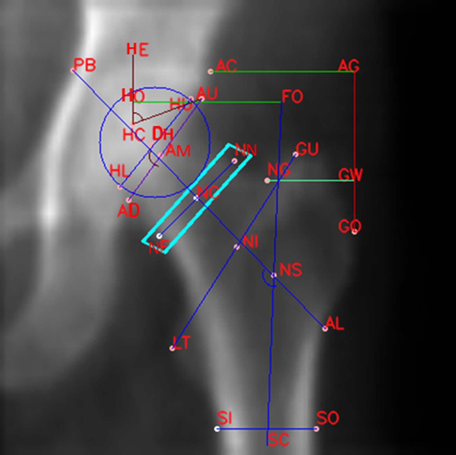
Geometric features measurements from a femur DXA image.

The geometry of hip plays a very important role in hip fracture. Evidence to date suggests an increase in FNL and an increase in the ratio of the FNL to the FNW ratio puts an individual at higher risk of hip fracture [41]. Studies of osteoporotic fractures have demonstrated that an increased HAL and NSA are associated with greater HFR independent of age and BMD [14 , 41]. An increase in ACW, an increase in the ratio of the FHD to the FNW, a lower trochanteric width, and a smaller SW indicate greater HFR [18, 41]. An increase in the CEA and PNA is associated with hip dysplasia and increased HFR [20 , 28–30]. A shorter FHO and ITD along with a wider HAL and GTAIICD are associated with greater HFR [29 , 32].

3.2 The proposed hip geometric features extraction algorithm

An overview of the automatic HGFs extraction technique from femur DXA images is provided in Fig. 2. The model localizes ALMs using ALMs={ALM_i|i=1,… ….n} to extract the HGFs. The algorithm starts with femur image acquisition using a DXA scanner. The image is denoised using a non-local means filter (NLMF). Then the hip in the image is segmented using a PLRF model. Hip contours are extracted from the segmented image to define structural ROIs. RRF localizes ALMs following the defined regional constraint for landmark localization. Finally, HGFs are extracted using the final set of ALMs.

Fig.2

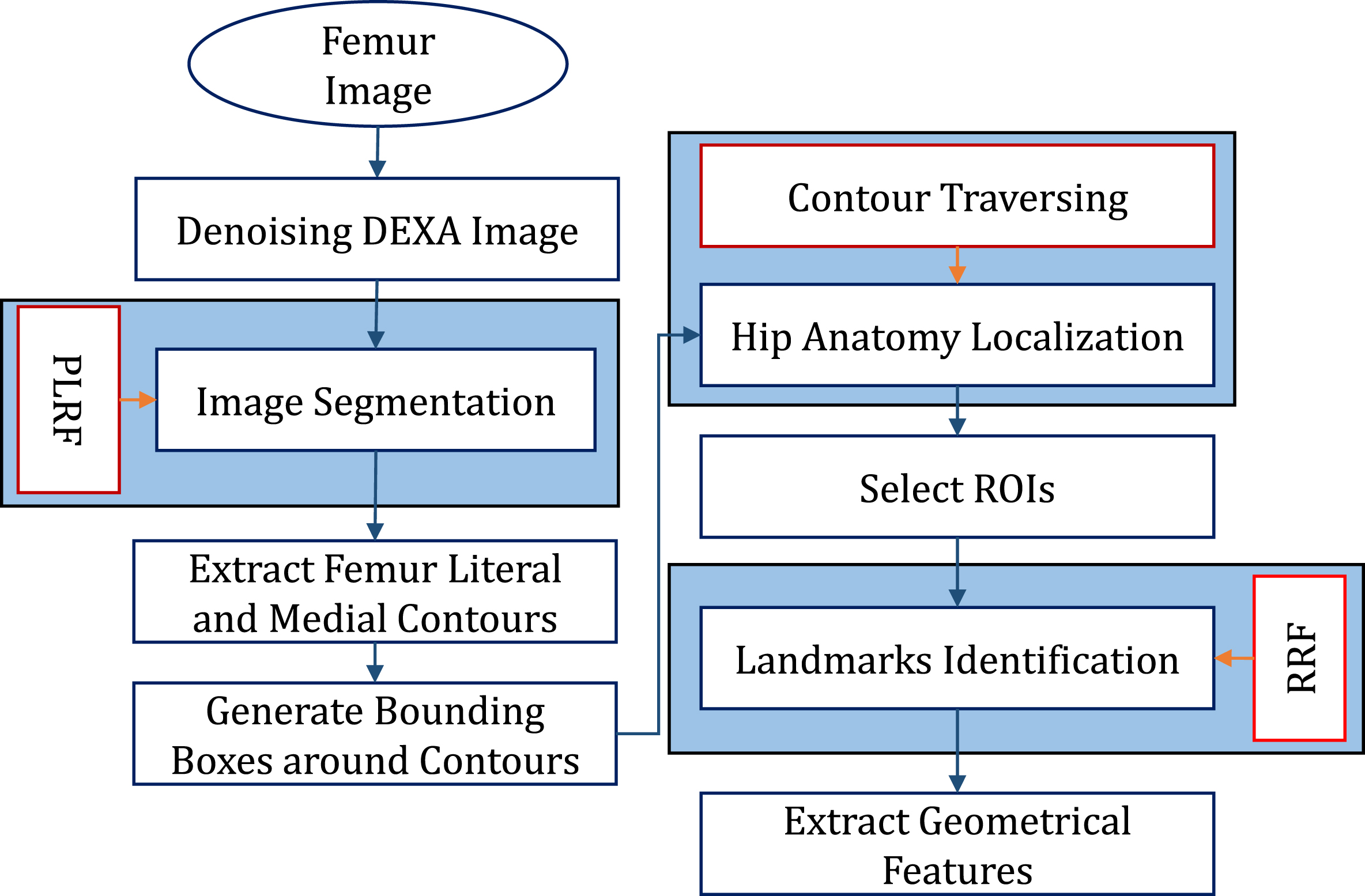
Hip geometric features extraction flowchart.

3.2.1 Femur image acquisition

To extract RF features for robust localization of ALMs and better visualization of HGFs, we need a clear and high-contrast DXA image. During a DXA scan, we get high energy (HE) and low energy (LE) images. These HE and LE images have very low contrast, so they are combined to yield a high contrast image called a BMD map (BMDMP). The BMDMP provides higher values in the bone region than the soft tissue region, so we are left with a clear and high contrast image. The BMDMP can be extracted from HE and LE images using the following equations: $BMDM P_{i} = \frac{R_{st} \times log \frac{H E_{i}}{H E_{0}} - log \frac{L E_{i}}{L E_{0}}}{u_{l} - u_{h} \times R_{st}},$ (1) $R_{st} = \frac{log \frac{L E_{0}}{\frac{1}{n} \sum_{i = 1}^{n} L E_{i}}}{log \frac{H E_{0}}{\frac{1}{n} \sum_{i = 1}^{n} H E_{i}}},$ (2) where u₁ and u_h in Equation 1 are known values (i.e., u_l = 0.4986 and u_h = 0.2563) from experiments with a specific LE X-ray and HE X-ray respectively. HE₀ and LE₀ are incident energy in the source X-ray, and HE_i and LE_i are the detector count at a specific scan location (i.e., pixel i). The R_st is first calculated using Equation 2, and then its value is used in BMDMP calculation using Equation 1.

3.2.2 Denoising the DXA image

To improve the quality of hip contour extraction from femur DXA images, the reduction of noise in both HE and LE images is often an essential preprocessing procedure. An NLMF denoises DXA images. More details about our previous work on DXA image denoising using an NLMF are available in [42, 43].

3.2.3 Image segmentation

PLRF is used to segment and extract hip contours from femur DXA images automatically. The PLRF differentiates hip bone pixels from the soft tissue or background pixels and then extracts the hip contour from the horizon of the hip object and the background. The contours define the fibrous structure of hip anatomy, which is used to select ROIs for the application of the RRF model. Fig. 3 demonstrates hip contours extraction from a femur DXA image via PLRF, starting with the femur data acquisition. Femur data are acquired from a DXA scan that produces HE and LE images. These HE and LE images are denoised using an NLMF. Then four new features maps are generated from the HE and LE images. Thus, a total of six features maps are available to train the PLRF model, which is later used to segment the hip captured from the femur DXA images.

Fig.3

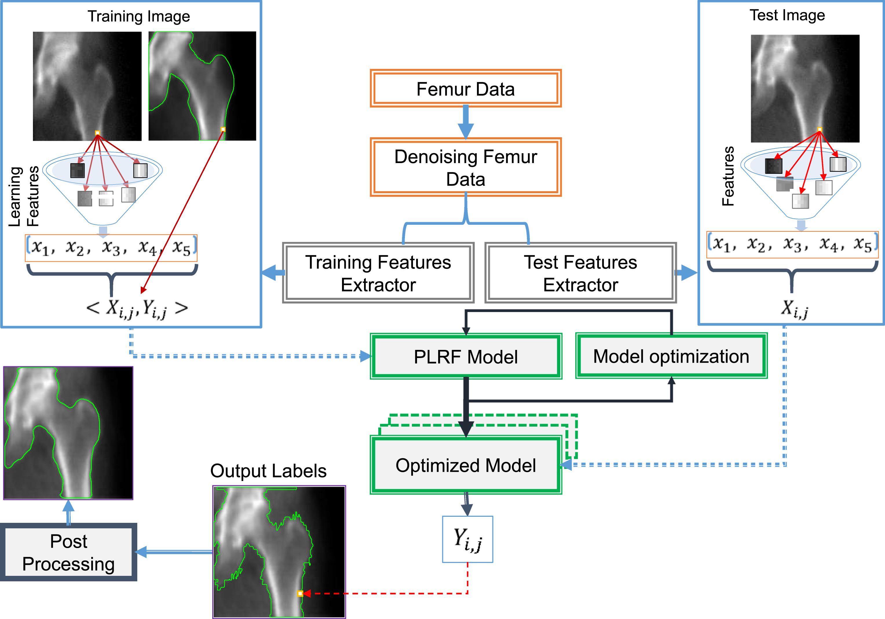
Overview of the pixel label random forest algorithm. Input training data are converted into features vectors that are then fed into the model. A trained model is used on the test data to predict a subject pixel label.

3.2.3.1 Pixel label random forest features representation

DXA produces HE and LE images. Our method generates four new features maps from these HE and LE images, which means information is being captured more effectively. The newly generated features maps include a BMDMP, a map showing the difference between LE and HE images (LHD), a local standard deviation of the BMDMP (LSTD_BMD), and a composite map (CI) [44]. Including the HE and LE images, a total of six features maps are available for the PLRF model.

The HE image is the first features map for the PLRF model available from a DXA scan. The quality of information in a DXA image depends on the attenuation contrast. The HE X-ray beam has more penetration power than an LE beam.

The LE image is the second features map and is also available from a DXA scan. Lowering the X-ray energy increases X-ray attenuation by tissue, thus producing a more informative image than the HE image [58].

The BMDMP is the third features map, and it is generated from the HE and LE images using Equation 1.

The LHD, the fourth features map, is generated as each pixel i of the HE image subtracted from each pixel i of the LE image as follows: $LHD = L E_{i} - H E_{i}$ (3)

This difference image usually contains useful information for femur segmentation. Because the air regions are more uniform than the bone or soft tissue areas, clear boundaries exist between the tissue and air regions. The LHD is used to identify the air regions, which are not included for classification.

The CI is the fifth features map generated. In LE images, the energy count in the soft tissue regions is greater than the count in bone. Therefore, a pixel belonging to the tissue region usually contains higher values than a pixel belonging to the bone region. Using the BMDMP and inverse of the LE image, tissue regions are suppressed to enhance the bone regions. We get a map with better contrast using the CI compared to the BMDMP and LE image. A CI better discriminates between bone and soft tissue regions compared to a BMDMP. The LE image and BMDMP are normalized first with a lower scale (a) and upper scale (b), and then they are used to form the CI as follows: ${BMDI}^{'} = a + \frac{BMD I_{i} - min (BMDI)}{max (BMDI) - min (BMDI)} (b - a),$ (4) ${LE}^{'} = a + \frac{L E_{i} - min (LE)}{max (LE) - min (LE)} (b - a),$ (5) $CI = {BMDI}^{'} * (1 - {LE}^{'})^{n},$ (6) where n is the power factor to suppress the tissue region. We use n = 3 for our CI feature generation. From experiments, we found that n = 3 is best for our data. A higher value n may affect a bone region. A lower value does not yield good suppression of the tissue region. Some of the composite images for different values of n are shown in Fig. 4.

The LSTD_BMD, the sixth features map, is generated using a 3x3 window with nine neighboring pixels. The standard deviation (STD) of each pixel is calculated in the BMDMP, and the local STD of the BMDMP is calculated using the following equation:

Fig.4

Composite images for different values of ‘n’ in Equation 6. (a) For n = 2; (b) for n = 3; (c) for n = 5; (d) for n = 7.

$LSTD_BMD = \sqrt{(\frac{1}{n} \sum_{i = 1, j}^{n} {(BMD I_{i} - μ_{j})}^{2})}$ (7) where i, n, and μ_j are an individual pixel, the total number of pixels, and the mean value in local window j respectively.

The STD can indicate a significant change in the image gradient present in a pixel neighborhood. A high value for STD indicates that the neighborhood pixel values could be spread far from the calculated mean. Inversely, a small STD indicates that the neighborhood pixel values have small variation to the calculated mean. A sudden change in image gradient will yield a significant STD. Usually, the border values between bone and soft tissue appear brighter due to a sudden change in BMD values. Some of the PLRF features maps are shown in Fig. 5.

Fig.5

Features maps. (a) High energy image; (b) low energy image; (c) map showing the difference between low and high energy images; (d) bone mineral density map; (e) composite map; (f) local standard deviation of the bone mineral density map.

3.2.3.2 Pixel label random forest design

The PLRF design of our ensemble model is composed of a set of n decision trees from k randomly selected subfeatures out of m features. The PLRF aggregates the votes from all the different decision trees to decide the final class label of the test subject. Each decision tree in the PLRF is implemented based on the standard CART algorithm [45]. The input features data set is represented in the form of a tuple (S, Y) as follows:

$f (S, Y) = (X_{1, j}, X_{2, j}, . . . . . . . . . . . . X_{m, j}, Y_{j})$ (8) where S is the features data set; X₁, X₂, … X_m represents an individual feature, and j represents the attribute value. The variable Y is a special discrete attribute designated as a class label (bone or soft tissue). A random function is used to select k out of m attributes from the training data set for an nth decision tree in the PLRF as follows: $f_{R} (S_{R, n}, Y_{R, n}) = (X_{1, j, n}, X_{2, j, n}, . . . . . . . . . . . . . X_{k, j, n}, Y_{j, n})$ (9)

The learning classification function f_R measures each attribute in a randomly selected subset S_R of features data set S to one of the predefined class labels Y_j,n in a subtree ‘n’ of the PLRF. The test image data are also represented in the form of features vectors as follows: $f (X) = (X_{1, j}, X_{2, j}, . . . . . . . . . . . . X_{m, j}),$ (10) $f_{R} (X_{R}) = (X_{1, j, n}, X_{2, j, n}, . . . . . . . . . . . . X_{k, j, n}),$ (11) where X₁, … X_k represents a features vector of pixel i in the image to be assigned a label by a tree ‘n’ in the model. The split optimization criterion used to measure node impurity in this model is the Gini Index.

Each tree in the PLRF needs stopping criteria as it splits down the tree with the training data. A tree terminates before it reaches maximum depth if some other matching criterion is met, for example, if the node samples are less than the specified threshold, all samples in the node belong to the same class, or no improvement is observed with the best split found compared to a random choice. We use 1% of the total data as a minimum count for training instances assigned to each leaf node of the tree to stop further splitting. If the count is less than the minimum number, then the node is taken as a final leaf node and further splitting is stopped. Trees are pruned to reduce the size of the PLRF model and improve classification accuracy. Cost complexity pruning determines the most significant splits in the model [45]. Nodes with anomalies and least classification performance are removed. The PLRF terminates when all the trees in the model are trained.

Training data is prepared by extracting a features data set from the denoised images. At each pixel i of jth training data set (features map/image), features are extracted to form a features vector X_i,j for that particular pixel, and the data set is assigned a class label (bone or soft tissue) denoted as Y_i,j. Thus, in a training data set, the components of vector X_i,j become attributes with dependent variables Y_i,j, and each training pixel i of jth training data set is made of a training pair (X_i,j, Y_i,j). Minimum (min) and maximum (max) values in the data are used to normalize it to a fixed range between 0 and 1.

To train the PLRF with n number from a sub-data-set of the training data set, each features vector belonging to pixel i represents pixel information, a class label, and a label of the sub-data-set. Random function is employed to assign a new label from the sub-data-set to each training pair (X_i,j, Y_i,j) with an extra dimension n (X_i,j,n, Y_i,j,n). We have N number of features vectors in sub-data-set n, and each vector has j number components called attributes (X_i,j,n) along with its class label (Y_i,j,n). Y is a dependent variable. Thus, each pixel i in a training data set for the nth tree is represented with a training pair (X_i,j,n, Y_i,j,n). In each PLRF tree, the best splitting attribute is selected based on the Gini Index criterion that best minimizes the Gini Index.

To prepare the test data set, each pixel i is represented by some features information along with the pixel position in the test image without the inclusion of a label. The test data sets are prepared by following the rules of each randomly created tree. To acquire a response for the input features vector in a particular tree using the PLRF model, it traverses all the nodes of the tree following the splitting criterion and threshold at each node until it reaches a leaf node. The training data vectors present in the leaves respond and place votes to predict the label for input data. Each tree in the model has its vector representation for a test subject and predicts a class label for it. Then by considering the predicted outcomes, the final votes are calculated. A testing subject (pixel) is assigned a class label based on the maximum votes received for a particular class. To resolve classification ties, the model uses a threshold value (e.g., above 50%) to vote for a particular class.

3.2.3.3 Postprocessing

The hip boundaries labeled by the PLRF are not smooth. The output of the PLRF is a binary image, as seen in Fig. 6(b). A binary smoothing filter is used to smooth hip boundaries as shown in Fig. 6(c) and Fig. 6(d). Binary smoothing removes small-scale noise in the shape while maintaining large-scale features.

Fig.6

Binary smoothing. (a) Object contours by pixel label random forest; (b) a binary image; (c) application of binary smoothing; (d) object contours after binary smoothing.

3.2.4 Contours processing

Contour features play a vital role in understanding an object’s anatomy. The maximum curvature points are most distinctive along a contour [49]. Our femur DXA image segmentation results in a binary image that is used to compute hip object contours. Hip contours are marked as being superior, inferior, or medial based on the boundaries of a white object against the black background. To identify the superior, inferior, and medial contours, the hip bone pixels are marked as background content, and surrounding tissues pixels are marked as an object. For better separation of the contours, a black frame is drawn around the binary image as shown in Fig. 7(b). The size of a contour and its position in the image define whether it is a superior, inferior, or medial contour. Each contour is enclosed in a bounding box (BX) according to its local minima and local maxima. The superior hip contour is enclosed in the top BX. The top BX contains anatomical structures such as the femur bone lateral edge, greater trochanter, superior edge of the femur neck, and superior edge of the femur head. The inferior hip contour is enclosed in the bottom BX, which includes the femur bone medial edge, hip ischium, lesser trochanter, and inferior edge of the femur head. The medial contour containing the pelvic brim of the hip is enclosed in the pelvic BX.

Fig.7

Contours extraction. (a) segmentation results using PLRF; (b) binary representation of segmented bone pixels (black) and soft tissue pixels (white); (c) medial and literal contours of the femur; (d) bounding boxes drawn around medial and literal contours of the femur.

3.2.5 Hip anatomy localization

The proposed algorithm uses hip contours features to obtain structural details about the femur and pelvis. The structural details of the femur and pelvis are used to select the ROIs for RRF implementation. A total of six ROIs are selected: the pelvic brim, femur head, femur neck, greater trochanter, lesser trochanter, and femur shaft regions.

3.2.5.1 Features representation

Feature extraction based on shape signature and polygonal approximation is done to collect details about the anatomical structure of the femur and pelvis. Shape signature is a one-dimensional function derived from shape boundary coordinates. The technique is robust to noise, translation, rotation, and scale invariance. A number of features represent points on the contours, which are extracted using triangle-area representation (TAR), the tangent angle function (TAF), the directional change map function (DCMF), and the distance threshold function (DTF).

Triangle-Area Representation: TAR captures the anatomical features of a contour and identifies them as being convex, concave, or a straight line. Triangles represent the contour points, and the area of the triangles is used to calculate the TAR signature [50, 51]. The curvature of the contour point (x_n, y_n) is measured using three consecutive points in a row: P_n–w_s(x_n–w_s, y_n–w_s), P_n (x_n, y_n), and P_n+w_s (x_n+w_s, y_n+w_s), where n ε [1, N], w_s ε [1, N/2–1], and N is even. The signed area of the triangle established by these points is given by: $TAR (n, t_{s}) = \frac{1}{2} | \begin{matrix} x_{n - w_{s}} & y_{n - w_{s}} & 1 \\ x_{n} & y_{n} & 1 \\ x_{n + w_{s}} & y_{n + w_{s}} & 1 \end{matrix} | .$ (12)

A positive TAR value means a convex point when traversing a contour in a counterclockwise direction. Similarly, negative and zero values of TAR mean concave and straight-line points, respectively. Some of the anatomical structures such as the acetabulum are represented with concave lines while a convex line represents others such as the lesser trochanter.

Tangent Angle Function: The TAF identifies the degree of convexity and concavity at a point in a contour. The tangent angle value of a point P_i (x_n, y_n) is determined by selecting two arbitrary points P₁ (X_(n - w), y_(n - w)) and P₂ (X_(n ₊ _w), y_(n ₊ _w)). The angle of inclination for the arbitrary points is computed as follows: $θ_{1} = \arctan (\frac{y_{(n)} - y_{(n - w)}}{x_{(n)} - x_{(n - w)}}),$ (13) $θ_{2} = \arctan (\frac{y_{(n + w)} - y_{(n)}}{x_{(n + w)} - x_{(n)}}),$ (14) where w is a small window to calculate the tangential angle. Before calculating the tangent angle, a contour is run through a low-pass filter with the appropriate bandwidth to decrease the noise effect. The inclination angle θ_n of P_i is defined as follows: $θ_{n} = 180^{0} - | θ_{2} - θ_{1} | .$ (15)

Directional Change Map Function: The DCMF incorporates information for a point from a contour stepping with Δ in a given direction in the left femur and right femur. This feature captures information on a contour point with relative change in the anatomical structure. The DCMF measures the response of every point on the contour, returning 1 or 0, using the following equations: $p_{i} = {\begin{matrix} 1, if p_{i}, x \geq p_{i - 1}, x and p_{i}, y \geq p_{i - 1}, y \\ 0, otherwise \end{matrix}, left femur,$ (16)

$p_{i} = {\begin{matrix} 1, if p_{i}, x \geq p_{i - 1}, x and p_{i}, y \geq p_{i - 1}, y \\ 0, otherwise \end{matrix}, right femur,$ (17)

Distance Threshold Function: The DTF follows the DCMF to extract details on anatomical structure for a specific location. A list of points L={p_i |i=1….n, p_i =1} is generated from already marked DCMF contour points. The distance d between two consecutive points P_i and P_i +1 is calculated using the following equation: $d_{i, \vec{i = 1 . . . n}} = \sqrt{{(p_{i + 1}, x - p_{i}, x)}^{2} + {(p_{i + 1}, y - p_{i}, y)}^{2}}$ (18)

3.2.5.2 Regions of interest selection

The hip superior, inferior, and medial contours enclosed in the top, bottom, and pelvic BXs are used to obtain the structural details. Automatic ROIs (as shown in Fig. 8) are generated based on different combinations of the abovementioned contour features using TAR, the TAF, the DCMF, or the DTF. The relationship between a structural landmark p_i and ROIs R is defined as, ${x R_{i} = x p_{i} + Δ x, y R_{i} = y p_{i} + Δ y}$ (19) where (xp_i, yp_i) is the location of a structural landmark p_i and (xR_i, yR_i) represents the center of ROI R_i. Δx and Δy are constants that represent the values of x and y offsets. The shaft ROI is selected as being 3 cm below the lesser trochanter. The femur narrow neck position is identified as being the shortest distance between the superior and inferior contours.

Fig.8

Generate automatic regions of interest. (a) Object contours are traversed to identify initial anatomical landmarks; (b) define region of interest for final localization of anatomical landmarks.

3.2.6 Anatomical landmarks localization using random forest

The desired ALMs are localized in the selected ROIs using RRF. Some of these ALMs are identified by RRF (e.g., the femur narrow neck upper and lower landmark points), while others are derived from the basic identification of the ALMs (e.g., the center of the femur neck). Each ALM represents an essential position on the pelvis and femur. The ALMs localization task is formulated as a multiclass classification problem. A feature set € (x) is used to represent a pixel x in the local region R_i. Then the RRF classifier is used to find the probability of pixel x and its relationship to landmark LM_i. A local maximum for the probability map is used to cast the final vote for a landmark.

3.2.6.1 Random forest features representation

To account for the miscellaneous nature of landmarks, we designed a pool of hybrid features that have short- and long-range contextual information [52, 53]. More relevant features are located for landmark detection in femur DXA images. The hybrid feature pool contains a Haar feature, a local feature that covers the short- and long-range contextual features.

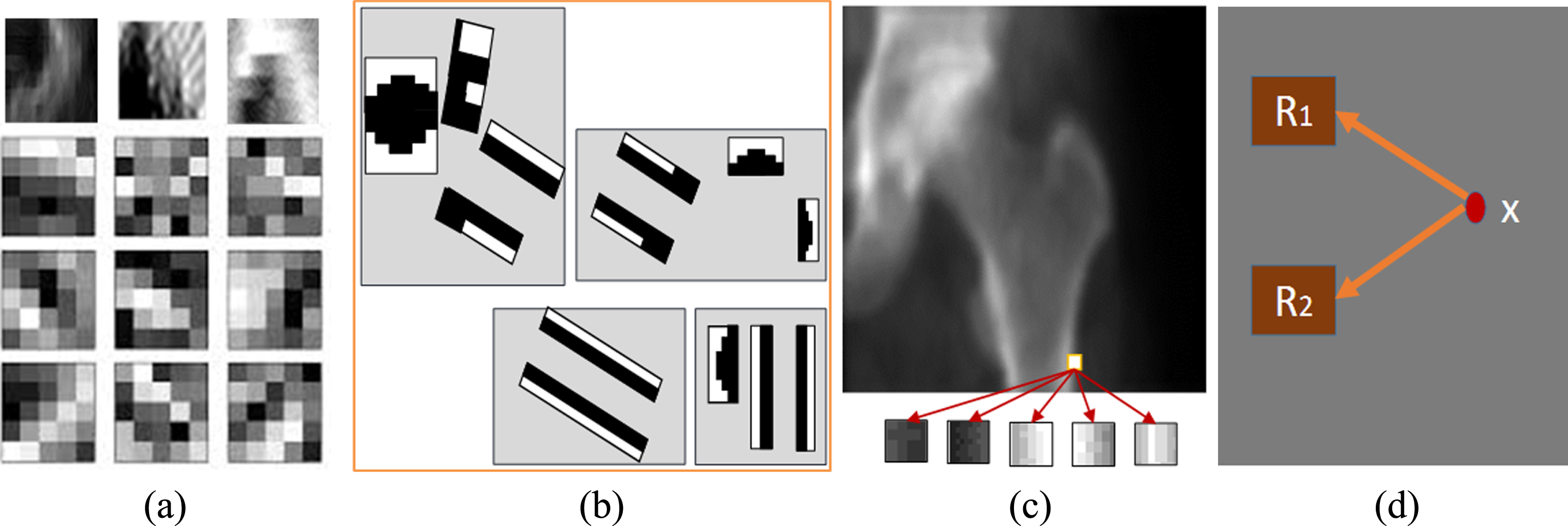
Convolutional Feature: Twelve different convolutional kernels are designed to obtain pixel information from an image, and they include local standard deviation (Equation 7), gradient ||g (x_k) ||, canny edge G (x_k), straight edges, curves, and corners. The convolutional feature, for a given pixel x, is sampled in a local region of size n×n using a BMDMP. Fig. 9(a) shows some of the local features calculated for a given pixel in an image.

Fig.9

Features representation for landmark detection. (a) Convolutional feature; (b) Haar feature; (c) local feature; (d) long-range contextual feature.

Haar Feature: Viola et al. used the Haar feature for face detection [54]. It is a common object detection technique. We used this feature for landmark detection with a hip object. The Haar feature is generated using a Haar-like filter, which is expressed as the difference of the sums of two adjacent rectangular regions at a specific location in a detection window of a given local patch size m×m. In this study, 13 Haar-like filters are used to generate a Haar feature as shown in Fig. 9(b). Different Haar features are designed and applied according to regional constraints. A Haar feature calculates the sum of the pixel intensities in the rectangular portion of the entire feature and the sum of the pixel intensities in the black portion. Features detection occurs very quickly because it is based on sum and threshold comparisons.

Local Feature: Some local information is used to represent a pixel in the image. The coverage of local information for a pixel holds an HE value, an LE value, a BMD value (calculated using Equation 1), a difference value of the LE and HE values (calculated using Equation 3), and a log ratio value of the HE to LE value as shown in Fig. 9(c).

Long-Range Contextual Feature: In 2009, Criminisi et al. [55] proposed a long-range contextual feature for 3-D organ localization. A similar approach is used here for 2-D femur DXA images. The problem with using only local features is that many different landmarks share very similar appearances, so it is hard to make a distinction between them. Thus, local contextual information is not sufficient. This is why global contextual information is also needed. Long-range contextual features use facts gathered from around the image. We divide the local region into smaller regions and incorporate long-range contextual information for a pixel x from the multiple regions as shown in Fig. 9(d). A defined threshold distance separates the regions. The long-range contextual information measures the offset Δ in a given direction with a relative mean difference between two regions. The long-range contextual information best covers details on anatomical structure. For a given pixel, the relative contextual feature f(x) is defined with two offset regions R₁ and R₂ as follows:. $f (x) = \sum_{x_{i} \in R_{1}} I (x_{i}) - \sum_{x_{j} \in R_{2}} I (x_{i}) .$ (20)

Thus, a pixel x is represented by a composite features vector € (x) in the form of convolutional, Haar, local, and long-range contextual features respectively.

3.2.5.2 Random forest framework

To handle the multidimensional feature pool € (x), we construct a collection of decision trees under a single ensemble of RF [56]. The RF classifier is robust and suitable for multiclass classification in the domain of medical imaging [55]. RF follows a randomized configuration of features selection to construct each tree with a suitable subset of features and then averages the results from all the trees. A terminal/leaf node represents the class label with a learned probability of landmarks as illustrated in Fig. 10. A binary distribution splits an internal node into its children. The splitting process stops when it reaches the leaf node. RF applies a general technique of bagging to learn a tree. Given a training set € (X)=x₁, x_2, …, x_n with a class label Y=y₁, y₂,..., y_n, the posterior probability is learned from features space X at each leaf node following the partition rule. Each tree randomly selects a sample from the features space.

Fig.10

Random forest framework. Leaves represent the learned probability p_i(LM_i) shown in green. Red arrows follow the prediction of x till it reaches the leaves. The final predicted probability Pr(LM_i) of a landmark LM_i is calculated as the mean distribution from all trees in the forest.

In the testing stage, a prediction is made about a pixel x using the feature € (x) of that pixel. Feature set € (x) of x is fed into the root node of each tree. Each tree splits the fed feature following the splitting rule until it reaches a leaf and returns posterior probabilities as an association of x to each landmark. The final decision is assembled based on a map generated as mean distributions of posterior probabilities at the leaves level from all trees. The posterior probability for x that belongs to a landmark LM_i is estimated by, $pr (L M_{i} | x) = \frac{1}{N} \sum_{j = 1}^{n} p_{j} (L M_{i} | \notin (x)),$ (21) where p_j(.) is the output from the Nth tree, and N is the number of trees in the forest. Local maxima of the probability map are used to finalize the final affiliation of a landmark LM_i to a point. Both GRF and RRF were tested individually to identify ALMs in femur DXA images. In GRF, every pixel in the image is tested along with its relation to an ALM point, whereas in RRF, only pixels inside an ROI are selected to check their relation to an ALM point.

3.2.7 Image resolution and geometric measurements

Image resolution is converted to a pixels-per-centimeter scale by calculating the diagonal density of pixels using the Pythagorean Theorem as follows: $d_{p} = \frac{\sqrt{w_{i}^{2} + h_{i}^{2}}}{\sqrt{w_{o}^{2} + h_{o}^{2}}},$ (22) where d_p is the number of pixels per centimeter, w_i, and h_i are the width and height of the displayed image respectively, and w_o and h_o are the dimensions of the scanned object. Landmark distance is used to calculate the length of a specific axis using the following equation: $L (cm) = \frac{\sqrt{(w_{1} - x_{2})^{2} + (y_{1} - y_{2})^{2}}}{d_{p}},$ (23) where L is the axis length, and (x₁,y₁) and (x₂,y₂) are two landmark points that represent an anatomical axis in an image.

The intersection of the derived anatomical axis forms the anatomical angles of the hip joints (e.g., the angle between the neck axis and shaft axis). An anatomical angle is calculated from the derived axes using the following steps:

Find the slope of anatomical axes m₁ and m₂.

Compute the angle of inclination of each line as follows: $θ_{i} = \tan^{- 1} m_{i} .$ (24)

Calculate the acute and obtuse angles using the inclination angles of m₁ and m₂.

4 Results

4.1 Data acquisition

In this work, we collected phantom and real femur DXA images using a DXA imaging system (OsteoPro MAX, B. M. Tech Worldwide Co., Ltd, Republic of Korea) with a maximum tube voltage and current of 76 keV and 1 mA respectively. A femur aluminum bar phantom (i.e., Lunar 1043) was used to obtain phantom images following the scanning protocol for a femur. A total area of 12.5 cm×12.5 cm was scanned with the DXA imaging system. The pixel resolution of the phantom and real femur DXA images was 1.3×2.6 mm² with 96×48 mm² in the field of view, and the image matrix size was 420×420. On a display image, every 33.6 pixels represents 1 cm area of the scanned object.

4.2 Evaluation and performance analysis

4.2.1 Evaluation

The proposed automatic HGFs technique was evaluated experimentally by comparing the extracted features to ground truths. For validation purposes, the femur phantom was first manually measured using a digital measurement tool called the Digital Caliper Deluxe Model. Then the phantom was scanned using the DXA imaging system, and HGFs were extracted using the proposed model. To generate ground truths for scanned data from a real human, ALMs were manually marked by three different radiology experts referencing the scanned image of a real human femur. ImageJ software was used to extract the HGFs digitally from the manually marked landmark points. The results extracted by the three experts were used in the mean statistical analysis to form the ground truths of the HGFs. The proposed automatic HGFs model results were then compared to the ground truths.

4.2.2 Performance analysis

Anatomical Landmark Identification: The manually marked landmark points created by the three different radiology experts were used in a mean statistical analysis (i.e., to find the mean of the three values about a landmark) to form the ground truths of the ALMs. The predictive performance of ALM detection was measured as an absolute difference between the ground truths and the automatically identified landmarks. Error related to a specific landmark LM_i was defined as, $EL M_{i} = \frac{\sum_{i = 1}^{n} | | L M_{gi} - L M_{pi} | |}{n},$ (25) where LM_g represents the ground truth value, and LM_p represents the predicted value of a specific landmark. The value of n is the total number of test images. The mean error of k landmark points was defined as, $ELM = \frac{\sum_{i = 1}^{k} EL M_{i}}{k} .$ (26)

We used a total of 13 ALMs to calculate the final error in ALM identification.

Hip Geometric Features: The performance analysis for HGFs was measured as an absolute difference between the values of the proposed model and the ground truths. The error rate and accuracy of each HGF was measured as follows: $E F_{i} = \frac{\sum_{i = 1}^{n} \sqrt{{(v_{gi} - v_{pi})}^{2}}}{n},$ (27) $Ac F_{i} (%) = 100 - \frac{E F_{i}}{v_{gi}} \times 100,$ (28) where v_g is the value of a ground truth, v_p is the predicted value, and EF is the error rate of a specific geometric feature. Ac_i represents the individual accuracy of a predicted feature. The overall average accuracy of the model was measured as follows: $Ac (%) = \frac{\sum_{i = 1}^{k} (Ac F_{i})}{k},$ (29) where k is the total number of geometric features.

Hip Anatomy Localization: The accuracy of hip anatomy localization was measured using the Jaccard index (JI). The crucial parts of the hip were enclosed in rectangular boxes. The area of the predicted rectangular box was compared to the ground truth using the following equation: $JI = \frac{Area of the intersection}{Area of union} .$ (30)

4.3 Segmentation results

Our design of the PLRF ensemble model was composed of a set of eleven decision trees with four randomly selected subset features from a total of six available features. The data (a total of 400 images) was divided into 80% for training and 20% for the test to validate the segmentation results. The input features for our PLRF model were an HE image, an LE image, a BMDMP, an LHD, an LSTD_BMD, and a CI. The model’s performance was checked using fivefold cross-validation. In each case, 20% of the reserved data was exchanged with another 20% of data from the training data set. Table 1 shows the performance analysis of the fivefold cross-validation. Segmentation accuracy was computed as the number of correctly segmented images from the test data set in five runs. The true positive rate (sensitivity) is the rate of correctly classified object pixels, whereas the true negative rate (specificity) is the rate of correctly classified pixels in the background. The false positive rate (FPR) and false negative rate (FNR) represent the pixels in the background region marked as object pixels and vice versa. An individual image was considered to be accurately segmented if both the image sensitivity and specificity were greater than 89%. Fig. 11 shows some of the segmentation results.

Fig.11

Pixel label random forest results. Boundaries using pixel label random forest (green) are compared with ground truths (red).

Table 1

Fivefold cross-validation and accuracy of pixel label random forest

Fold	Segmentation Accuracy (%)	Sensitivity (%)	FPR (%)	Specificity (%)	FNR (%)
1	97	98	5	95	2
2	93	95	7	93	5
3	88	90	11	89	10
4	92	92	9	91	8
5	95	94	7	93	6
Mean	93	∼94	7.8	92.2	∼6

4.4 Hip anatomy localization results

Hip anatomy localization and region-based RF implementation improved the performance of HGFs extraction. Hip anatomical structures were localized with a very high mean JI of 0.9862. The results of hip anatomy localization are shown in Table 2. The JI yields a value between 0 and 1. A value of 0 means no similarity while 1 means 100% similarity between the predicted and ground truth results. The ground truths are generated manually, as each anatomic structure in hip is enclosed in a rectangular box. Out of the 200 tested images, only 4 images were detected with bad contours. The JI value in those four images was not robust, so the contours were corrected manually. We had the option to manually correct bad contours.

Table 2
Hip anatomy localization

Hip Anatomy JI

Femur neck 0.989

Pelvic brim 0.978

Greater trochanter 0.992

Lesser trochanter 0.973

Femur shaft 0.999

Mean 0.9862

Hip Anatomy	JI
Femur neck	0.989
Pelvic brim	0.978
Greater trochanter	0.992
Lesser trochanter	0.973
Femur shaft	0.999
Mean	0.9862

4.5 Anatomical landmark detection results

A data set of 400 images was used to train and test the RF classifier. Out of these images, 250 were used for training and 150 were for the independent test. A total of 17 values were extracted for local and convolutional features. The local patch size for a Haar feature was 25×25. The long-range contextual features were computed in a local region of 25×25 with a size offset of 9×9 for R₁ and R₂. In the case of GRF, the regional window size was set to 40×30 around a pixel x, and the size of R₁ and R₂ was set to 16×16. Each model learned from 250 training images with 15 decision trees and 10 random subset features selected out of feature pool € (x). We conducted experiments to study the effect of each feature on the RRF model. The ALM detection results for the proposed system compared to the manual annotations are provided in Table 3. The table represents a mean difference in millimeters between the detected landmarks and ground truths. Fig. 12 illustrates a comparison of landmark detection using either GRF or RRF to the ground truth results. The overall landmark prediction error for the RRF and GRF systems was 2.5 ± 0.6 mm and 5.72±2.99 mm respectively.

Fig.12

Landmark validation. Landmarks with green color represent ground truths, whereas red items are predicted landmarks by regional random forest and blue items are landmarks predicted by global random forest.

Table 3

Mean difference of landmark detection compared to ground truths. The difference between detected landmarks and ground truths is calculated in millimeter

Landmarks	Features
	RRF					GRF
	Convolutional	Local	Haar	Long range	Convolutional, Local, Haar, Long range	Convolutional, Local, Haar, Long range
1	7.6521	7.7850	8.2908	5.5997	3.6928	7.2576
2	4.1862	6.0872	6.7865	5.0557	3.4328	8.4852
3	3.1268	4.0395	4.5723	4.6287	2.4148	5.1323
4	3.5670	3.8680	6.7295	6.0994	1.9980	6.1819
5	6.2405	5.6601	6.9387	5.2807	2.9925	4.9112
6	6.7687	6.7687	7.3038	4.5793	3.0145	9.9984
7	2.4590	3.4258	4.2438	5.0010	1.9089	3.1282
8	3.6725	4.7693	5.0443	6.0882	2.8475	7.7585
9	2.0998	2.4236	3.2718	4.2110	2.0776	11.4555
10	2.6602	2.6584	3.0403	2.8781	2.6574	2.8459
11	1.4986	1.7768	2.3121	3.2010	1.3247	3.3843
12	1.9821	1.9863	2.0423	3.0882	1.9584	2.0012
13	1.9899	2.0603	3.0223	4.0013	1.7584	1.8204
Average	3.6849	4.1007	4.8922	4.5932	2.4676	5.7200

4.6 Results of DXA phantom

The aluminum phantom was scanned with different orientations and different sizes of acrylic sheets over it to increase the data size. Data augmentation was used to further increase the size of the data. Data augmentation was performed using different transformations such as shifting, object resizing with linear regression, and rotation relative to the center of the image. For validation purposes, the phantom was physically measured by three different experts using a digital caliper. The mean value for the three different measurements was taken as the ground truth. Fig. 13 shows some of the phantom results. Table 4 provides a comparison between the RF models and ground truth results.

Fig.13

Phantom validation. (a) Aluminum phantom of the femur; (b) scanned aluminum phantom and measured geometric features.

Table 4

Femur phantom manual results compared to proposed system results. Reference measurements represent the mean of phantom results measured by three different experts. Length and width parameters and their error are measured in centimeter whereas an angle is measured in degrees

Feature	Reference Measurements	Proposed System RRF			Proposed System GRF
Feature	Reference Measurements	Measured	Error rate	Accuracy (%)	Measured	Error rate	Accuracy (%)
FNW (cm)	2.75	2.64	0.11	96.00	2.46	0.29	89.45
FNL (cm)	3.65	3.55	0.10	97.26	4.51	0.86	76.42
HAL (cm)	10.25	9.61	0.64	93.76	9.69	0.56	94.54
NSA°	126.00	125.00	1.00	99.21	140.00	14.00	88.89
SW (cm)	3.05	3.12	0.07	97.70	3.14	0.09	97.05
FHD (cm)	3.62	3.48	0.14	96.13	4.85	1.23	66.02
FHO (cm)	3.85	4.06	0.21	94.55	5.32	1.47	61.82
GTW (cm)	3.94	3.89	0.05	98.73	3.28	0.66	83.25
ITD (cm)	7.55	7.52	0.03	99.60	8.01	0.46	93.90
GTAIICD (cm)	6.00	5.74	0.26	95.67	8.8	2.8	53.33
ACW (cm)	3.94	3.76	0.18	95.43	4.68	0.74	81.22
CEA°	31.00	29.38	1.62	94.77	23.32	7.68	75.22
PNA°	74.00	79.87	5.87	92.07	86.75	12.75	82.77
Average	21.51	21.66	0.79	96.22	23.45	3.35	80

4.7 Results of human data

ImageJ software was used to generate the ground truths for data on a real human case. Measurements made by three different experts were used to calculate a mean, and STD statistical analysis was done to compute the accuracy of the proposed model results. A detailed analysis of three selected cases is presented in Table 5 and Table 6 using RRF and GRF respectively. The final accuracy of the RRF and GRF techniques are presented in Table 7 as a summary of mean and STD statistical analysis for 150 real human test cases. The value of each row in the accuracy column of a table represents the individual accuracy of each geometric feature whereas the value at the end of an accuracy column in a table represents the final accuracy of the proposed model. In addition, the receiver operating characteristic (ROC) based data analysis was also conducted. The performance of RRF and GRF on test data was evaluated using a ROC curve as presented in Fig. 14. Some of the test case results from the proposed model are presented in Fig. 15 and Table 8.

Fig.14

Receiver operating characteristic curve for regional vs. global random forest.

Fig.15

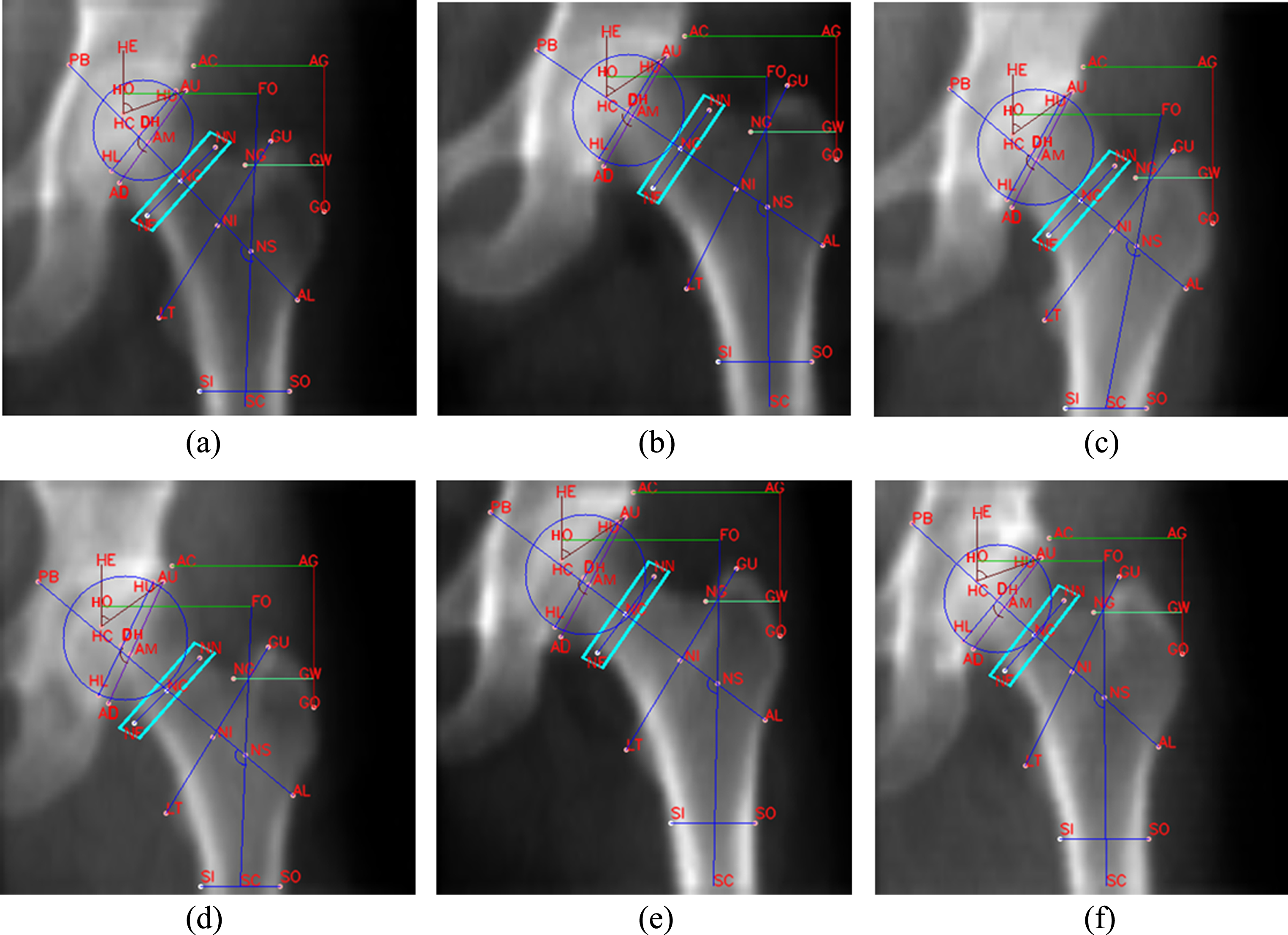
Hip geometric features.

Table 5

Real human femur results of the proposed regional random forest system for three different cases compared to ground truths generated using ImageJ. The ground truths are used to calculate the error rate (E) and accuracy (Ac) against the predicted results. The results are presented in centimeters in cases of length and width and degrees in the case of an angle

Features	Case 1				Case 2				Case 3
Features	ImageJ	RRF	E	Ac (%)	ImageJ	RRF	E	Ac (%)	ImageJ	RRF	E	Ac (%)
FNW(cm)	2.89	2.78	0.11	96.19	2.21	2.57	0.36	83.71	2.47	2.35	0.12	95.14
FNL(cm)	3.61	3.56	0.05	98.61	3.39	3.31	0.08	97.64	2.45	2.54	0.09	96.33
HAL(cm)	10.46	10.07	0.39	96.27	9.98	9.64	0.34	96.59	9.25	9.44	0.19	97.95
NSA°	121.9	125	3.1	97.46	126.45	129	2.55	97.98	128	133	5	96.09
SW(cm)	2.54	2.6	0.06	97.64	2.72	2.79	0.07	97.43	2.73	2.76	0.03	98.90
FHD(cm)	4.18	4.04	0.14	96.65	3.85	3.35	0.5	87.01	3.26	3.12	0.14	95.71
FHO(cm)	4.88	4.21	0.67	86.27	4.99	4.23	0.76	84.77	3.86	3.48	0.38	90.16
GTW(cm)	3.41	3.08	0.33	90.32	2.81	2.65	0.16	94.31	3.07	3.11	0.04	98.70
ITD(cm)	5.97	6.2	0.23	96.15	5.21	5.56	0.35	93.28	6.22	6.4	0.18	97.11
GTAIICD(cm)	4.83	4.73	0.1	97.93	4.91	5	0.09	98.17	4.79	4.64	0.15	96.87
ACW(cm)	4.38	4.12	0.26	94.06	3.98	3.79	0.19	95.23	3.56	3.32	0.24	93.26
CEA°	31.45	36.65	5.2	83.47	29.01	26	3.01	89.62	28.34	31.05	2.71	90.44
PNA°	83.9	75.11	8.79	89.52	77.99	82.58	4.59	94.11	71	78.54	7.54	89.38
Average	21.88	21.70	1.49	93.89	21.35	21.57	1.00	93.07	20.69	21.83	1.29	95.08

Table 6

Real human femur results using global random forest for three different cases compared to ground truths generated using ImageJ. The ground truths are used to calculate the error rate (E) and accuracy (Ac) against the predicted results. The results are presented in centimeters in cases of length and width and degrees in the case of an angle

Features	Case 1				Case 2				Case 3
Features	ImageJ	GRF	E	Ac (%)	ImageJ	GRF	E	Ac (%)	ImageJ	GRF	E	Ac (%)
FNW(cm)	2.89	3.52	0.63	78.20	2.21	2.47	0.26	88.24	2.47	2.25	0.22	91.09
FNL(cm)	3.61	3.46	0.15	95.84	3.39	4.21	0.82	75.81	2.45	2.74	0.29	88.16
HAL(cm)	10.46	10.17	0.29	97.23	9.98	9.15	0.83	91.68	9.25	10.12	0.87	90.59
NSA°	121.9	127	5.10	95.82	126.45	135	8.55	93.24	128	131	3.00	97.66
SW(cm)	2.54	3.40	0.86	66.14	2.72	2.86	0.14	94.85	2.73	2.79	0.06	97.80
FHD(cm)	4.18	3.34	0.84	79.90	3.85	3.26	0.59	84.68	3.26	2.89	0.37	88.65
FHO(cm)	4.88	5.43	0.55	88.73	4.99	4.21	0.78	84.37	3.86	3.17	0.69	82.12
GTW(cm)	3.41	4.05	0.64	81.23	2.81	2.25	0.56	80.07	3.07	2.78	0.29	90.55
ITD(cm)	5.97	7.32	1.35	77.39	5.21	5.78	0.57	89.06	6.22	5.24	0.98	84.24
GTAIICD(cm)	4.83	3.21	1.62	66.46	4.91	5.87	0.96	80.45	4.79	5.74	0.95	80.17
ACW(cm)	4.38	3.85	0.53	87.90	3.98	3.67	0.31	92.21	3.56	3.31	0.25	92.98
CEA°	31.45	42.65	11.2	64.39	29.01	24	5.01	82.73	28.34	35.15	6.81	75.97
PNA°	83.9	70.2	13.7	83.67	77.99	84.59	6.6	91.54	71	77.94	6.94	90.23
Average	21.88	22.12	2.88	81.76	21.35	22.10	2.00	86.84	20.69	21.93	1.67	88.48

Table 7

Comparison of mean statistics for 150 real human images using regional or global random forest to ground truths generated using ImageJ. The error rate shows an absolute difference between the measured results and ground truths. The results are presented in centimeters in the cases of length and width and degrees in the case of an angle

Features	Reference Mean(±STD)	RRF Predicted Mean(±STD)	GRF Predicted Mean(±STD)	Error Rate Mean(±STD)		Accuracy (%)
Features	Reference Mean(±STD)	RRF Predicted Mean(±STD)	GRF Predicted Mean(±STD)	RRF	GRF	RRF	GRF
FNW(cm)	2.82(0.46)	2.77(0.34)	2.54(0.99)	0.05(0.12)	0.28(0.53)	98.23	90.07
FNL(cm)	3.45(0.52)	3.24(0.60)	3.87(0.97)	0.21(0.08)	0.42(0.45)	93.91	87.83
HAL(cm)	9.86(0.92)	9.72(0.96)	10.65(1.36)	0.14(0.04)	0.79(0.44)	98.58	91.99
NSA°	125.45(7)	129(9.00)	132.75(12)	3.55(2.00)	7.3(5.00)	97.17	94.18
SW(cm)	2.66(0.15)	2.72(0.18)	3.02(0.93)	0.06(0.03)	0.36(0.78)	97.74	86.47
FHD(cm)	3.76(0.34)	3.5(0.57)	3.45(0.94)	0.26(0.23)	0.31(0.60)	93.09	91.76
FHO(cm)	4.28(0.6)	3.97(0.80)	3.56(1.40)	0.31(0.20)	0.72(0.80)	92.76	83.18
GTW(cm)	3.10(0.32)	2.95(0.50)	3.7(0.85)	0.15(0.18)	0.6(0.53)	95.16	80.65
ITD(cm)	5.80(1.3)	6.05(1.06)	6.68(2.60)	0.25(0.24)	0.88(1.30)	95.69	84.83
GTAIICD(cm)	4.84(0.77)	4.79(0.87)	5.72(1.23)	0.05(0.1)	0.88(0.46)	98.97	81.82
ACW(cm)	3.97(0.23)	3.74(0.56)	3.61(1.01)	0.23(0.33)	0.36(0.78)	94.21	90.93
CEA°	29.60(6.5)	31.23(8.5)	38.43(13.20)	1.63(2.00)	8.83(6.70)	94.49	70.17
PNA°	77.63(8.86)	80.49(9.9)	70.33(16.02)	2.86(1.04)	7.3(7.16)	96.32	90.60
Average	21.32(2.15)	21.86(2.60)	22.18(4.12)	0.53(0.45)	0.85(1.96)	95.87	86.50

Table 8

Measurements for each geometric feature shown in Fig. 15

Index	Image
Index	a	b	c	d	e	f
FNW(cm)	2.75	2.79	2.63	2.48	2.62	2.48
FNL(cm)	2.84	3.89	2.76	3.39	3.45	3.13
HAL(cm)	8.39	9.65	8.71	10.02	9.62	9.07
NSA°	132	128	144	140	128	132
SW(cm)	2.89	2.68	2.65	2.71	2.71	2.53
FHD(cm)	3.10	3.08	3.31	3.25	3.48	3.27
FHO(cm)	3.56	4.35	3.90	3.66	4.42	3.53
GTW(cm)	2.44	2.80	2.41	2.47	2.59	2.86
ITD(cm)	6.11	6.50	6.01	5.75	6.28	6.54
GTAIICD(cm)	3.93	4.64	3.90	4.35	4.46	4.11
ACW(cm)	3.34	3.34	3.57	3.59	3.82	3.61
CEA°	31.93	36.28	36.02	31.86	33.35	35.29
PNA°	75.74	81.16	75.92	68.57	82.86	78.10

5 Discussion

The study shows that the RF classifier was an effective method for locating ALMs in femur DXA images. The constraints of local processing drastically increase the performance of RF and landmark detection. To improve the quality of X-ray images, the reduction of noise could be an essential preprocessing procedure [60 –65]. Different features and their combination have an effect on RF classification and voting for a landmark. Contour features play a very crucial role in ROI selection for local processing and precise HGFs extraction. Contour processing can effectively be used to extract the structural details of a hip with a very high JI of 0.9962. Extraction of the hip contours using PLRF with an accuracy of 93% is the gateway for hip anatomy localization and automatic ROIs selection. Landmark and HGFs detection was performed with more relevant features captured in femur DXA images. The features in the current study were designed to account for the nature and behavior of DXA data.

A number of studies have supported automatic landmark detection to overcome the manual marking of landmarks in X-ray images [47 , 55]. In 2016, Cheng et al. [58] used RF to localize landmarks in dual-energy dental radiographs, which are helpful in assessing the evidence of osteoporosis. Their proposed method achieved an average detection error of 2.9 mm. Our proposed model of ALM detection from femur DXA images using RRF with an effective combination of features achieved an average detection error of 2.46 mm. The most up-to-date studies have discussed the significance of the structural geometry of bones and the role of structural geometry in the risk of fracture [3 , 59]. All recent studies have either extracted geometric features manually or extracted them using semiautomatic, hand-operated HSA software. The current model extracts most HGFs in a fully automatic way with a higher accuracy of 96.22%.

The automatic prediction of HGFs was extensively investigated in this study by considering different parameters and feature extraction from femur DXA images. The performance of our approach was substantially increased with optimal testing. We have shown that a PLRF classification with appropriate features provides an effective way to segment and extract contours from DXA images. RF does not need any specialized hardware for training and prediction. It is a powerful classifier compared to other conventional classifiers such as support vector machine, neural networks, the k-nearest neighbors (KNN) algorithm, logistic regression, and naive Bayes [57]. Manual correction of contours was performed for only 4 images out of 200. In addition, the overall accuracy of 93% for hip segmentation and contours extraction makes RF one of the most suitable techniques for the segmentation of DXA images. An ensemble RF is less proven for overfitting compared to a single decision tree and other conventional classification techniques. The features for contour processing show very high performance concerning anatomy localization and automatic region selection in femur DXA images. The local region bounding search for a landmark point increased the robustness of our model. To the best of our knowledge, this has been the first study conducted for fully automatic HGFs extraction from femur DXA images. The high accuracy of 95.87% and 96.22% for real and phantom data, respectively, makes this approach suitable for the automatic collection of HGFs.

6 Conclusion

Roentgen’s discovery of X-ray changed people’s view of the world in the health-care domain. Researchers dealing with human health are continuously struggling to procure more useful information from radiological images [60 –77]. In this paper, we proposed a new method for automatic HGFs extraction from femur DXA images. An RRF classifier was used to localize landmarks in femur DXA images and extract HGFs. These rich features were then used to uncover the appearance of landmarks. This study evaluated the RF model’s ability in landmark detection using global and local constraints. RRF performed well in terms of accuracy compared to GRF. The algorithm was fast and robust due to the local search constrained by the ALMs. The proposed model compiled femur DXA images for HGFs extraction with a high accuracy of 95.87% and 96.22% for real and phantom data respectively. One limitation of this approach is the requirement for the optimal supervised selection of features. Although the latest deep learning methods can learn features from original data, a significant amount of training data is required. We plan to adopt deep learning approaches for HGFs extraction from DXA images shortly since a larger data set is being built up.

References

Karlsson

K.M.

, Sernbo

, Obrant

K.J.

et al. Femoral neck geometry and radiographic signs of osteoporosis as predictors of hip fracture, Bone 18(4) (1996), 327–330.

Faulkner

K.G.

, Cummings

S.R.

, Black

et al., Simple measurement of femoral geometry predicts hip fracture: The study of osteoporotic fractures, Journal of Bone and Mineral Research 8(10) (1993), 1211–1217.

Lee

D.H.

, Jung

K.Y.

, Hong

A.R.

et al., Femoral geometry, bone mineral density, and the risk of hip fracture in premenopausal women: A case control study, BMC Musculoskeletal Disorders 17(1) (2016), 17–42.

Semanick

L.M.

, Beck

T.J.

, Cauley

J.A.

et al., Association of body composition and physical activity with proximal Femur geometry in middle-aged and elderly Afro-Caribbean men, Calcified Tissue International 77(3) (2005), 160–166.

Petit

M.A.

, Beck

T.J.

, Shults

et al., Proximal Femur bone geometry is appropriately adapted to lean mass in overweight children and adolescents, Bone 36(3) (2005), 568–576.

Bainbridge

K.E.

, Sowers

, Lin

, Harlow

S.D.

, Risk factors for low bone mineral density and the 6-year rate of bone loss among premenopausal and premenopausal women, Osteoporosis International 15(6) (2004), 439–446.

Margolis

K.L.

, Ensrud

K.E.

, Schreiner

P.J.

, Tabor

H.K.

, Body size and risk for clinical fractures in older women, Annals of International Medicine 133(2) (2000), 123–127.

Moro

van der Meulen

M.C.H.

, Kiratli

B.J.

, et al., Body mass is the primary determinant of midfemoral bone acquisition during adolescent growth, Bone 19(5) (1996), 519–526.

Goulding

, Taylor

R.W.

, Jones

I.E.

et al., Overweight and obese children have low bone mass and area for their weight, International Journal of Obesity 24 (2000), 627–632.

10.

Goulding

, Jones

I.E.

, Taylor

R.W.

et al., More broken bones: A 4-year double cohort study of young girls with and without distal forearm fractures, Journal of Bone and Mineral Research 15(10) (2000), 2011–2018.

11.

Skaggs

D.L.

, Loro

M.L.

, Pitukcheewanont

, Tolo

, Gilsanz

, Increased body weight and decreased radial cross-sectional dimensions in girls with forearm fractures, Journal of Bone and Mineral Research 16(7) (2001), 1337–1342.

12.

Shaar

L.A.

, Nabulsi

, Maalouf

et al., Effect of vitamin D replacement on Hip structural geometry in adolescents: A randomized controlled trial, Bone 56(2) (2013), 296–303.

13.

Beck

T.J.

, Hip structural analysis (HSA) program, Johns Hopkins University, School of Medicine, Department of Radiology and Radiological Sciences, North Caroline, U.S, (2002).

14.

Leslie

W.D.

, Lix

L.M.

, Morin

S.N.

et al., Hip axis length is a FRAX-and bone density-independent risk factor for hip fracture in women, The Journal of Clinical Endocrinology & Metabolism 100(5) (2015), 2063–2070.

15.

Lindner

, Bromiley

P.A.

, Ionita

M.C.

, Cootes

T.F.

, Robust and accurate shape model matching using random forest regression-voting, IEEE Transactions on Pattern Analysis and Machine Intelligence 37(9) (2015), 1862–1874.

16.

Schumann

, Tannast

, Nolte

L.P.

, Zheng

, Validation of statistical shape model based reconstruction of the proximal Femur— a morphology study”. Medical Engineering and Physics 32(6) (2010), 638–644.

17.

Deshmukh

T.R.

, Kuthe

A.M.

, Ingole

D.S.

, Thakre

S.B.

, Prediction of Femur bone geometry using anthropometric data of Indian population: A numerical approach, Journal of Medical Science 10(1) (2010), 12–18.

18.

Partanen

, Jamsa

, Jalovaara

, Influence of the upper Femur and pelvic geometry on the risk and type of Hip fractures, Journal of Bone and Mineral Research 16(8) (2001), 1540–1546.

19.

Viradia

N.K.

, Berger

A.A.

, Dahners

L.E.

, Relationship between width of greater trochanters and width of iliac wings in trochanteric bursitis, American Journal of Orthopedics (Belle Mead, NJ) 40(9) (2011), E159–62.

20.

Pun

, Hip dysplasia in the young adult caused by residual childhood and adolescent-onset dysplasia, Current Reviews in Musculoskeletal Medicine 9(4) (2016), 427–434.

21.

Gala

J.C,

Clohisy

and P.E.

Beaule,

, Hip Dysplasia in the Young Adult, The Journal of Bone and Joint Surgery 98(1) (2016), 63–73.

22.

Petit

A.M.

Mckay

H.A.

, Mackelvie

K.J.

, et al., A randomized school-based jumping intervention confers site and maturity-specific benefits on bone structural properties in girls: A Hip structural analysis study, Journal of Bone Miner Research 17(3) (2002), 363–372.

23.

Ferry

, Lespessailles

, Rochcongar

et al., Bone health during late adolescence: Effects of an 8-month training program on bone geometry in female athletes, Joint Bone Spine 80(1) (2013), 57–63.

24.

Forwood

M.R.

, Bailey

D.A.

, Beck

T.J.

et al., Sexual dimorphism of the femoral neck during the adolescent growth spurt: A structural analysis, Bone 35(4) (2004), 973–981.

25.

Beck

T.J.

, Looker

A.C.

, Mourtada

et al., Age trends in Femur stresses from a simulated fall on the Hip among men and women: Evidence of homeostatic adaptation underlying the decline in Hip BMD, Journal of Bone and Mineral Research 21(9) (2006), 1425–1432, doi: 10.1359/jbmr.060617.

26.

Kaptoge

, Beck

T.J.

, Reeve

et al., Prediction of incident Hip fracture risk by Femur geometry variables measured by Hip structural analysis in the study of osteoporotic fractures, Journal of Bone and Mineral Research 23(12) (2008), 1892–1904 doi: 10.1359/jbmr.080802.

27.

LaCroix

A.Z.

, Beck

T.J.

, Cauley

J.A.

et al., Hip structural geometry, and incidence of hip fracture in postmenopausal women: What does it add to conventional bone mineral density, Osteoporosis International 21(6) (2010), 919–929, doi: 10.1007/s00198-009-1056-1.

28.

Lane

N.E.

, Nevitt

M.C.

, Osteoarthritis, bone mass, and fractures: How are they related? Arthritis & Rheumatology 46(1) (2002), 1–4.

29.

Burger

, van Daele

P.L.A.

Odding

, et al., Association of radiographically evident osteoarthritis with higher bone mineral density and increased bone loss with age, The Rotterdam Study, Arthritis & Rheumatology 39(1) (1996), 81–86.

30.

Arden

N.K.

, Nevitt

M.C.

, Lane

N.E.

et al., Osteoarthritis and risk of falls, rates of bone loss and osteoporotic fractures, Arthritis & Rheumatism 42(7) (1999), 1378–1385.

31.

G.I.

, Lim

M.J.

, Proximal Hip geometry and Hip fracture risk assessment in a Korean population, Osteoporosis International 22(3) (2011), 803–807.

32.

Shbeeb

M.I.

, Matteson

E.L.

, Trochanteric bursitis (greater trochanter pain syndrome), In Mayo Clinic Proceedings 71(6) (1996), 565–569.

33.

Brunner

L.C.

, Oates

L.E.

, Kuo

T.Y.

, Hip fractures in adults, American Family Physician 67(3) (2003), 537–542.

34.

Boudreaux

R.D.

, Sibonga

J.D.

, Advanced Hip Analysis: Simple Geometric Measurements Predict Hip Fracture Beyond Bone Mineral Density, Texas Orthopaedic Journal 1(2) (2015), 109–122.

35.

Karlamangla

A.S.

, Connor

E.B.

, Young

, Greendale

G.A.

, Hip fracture risk assessment using composite metrics of femoral neck strength: The Rancho Bernardo study, Osteoporosis International 15(1) (2004), 62–70.

36.

Cardadeiro

, Baptista

, Janz

K.F.

et al., Pelvis width associated with bone mass distribution at the proximal Femur in children 10–11 years old, Journal of Bone and Mineral Metabolism 32(2) (2014), 174–183.

37.

Souza

A.D.

, Ankolekar

V.H.

, Padmashali

et al., Femoral Neck Anteversion and Neck Shaft Angles: Determination and their Clinical Implications in Fetuses of Different Gestational Ages, Malaysian Orthopedic Journal 9(2) (2015), 33–36.

38.

Abramoff

M.D.

, Magallanes

P.j.

, Ram

S.J.

, Image processing with ImageJ, Biophotonics International 11(7) (2004), 36–42.

39.

Lakshmi

, Sumit

, Tuhin

, Pratima

, A digital image analysis method for measuring femoral neck shaft angle and anteversion angle: A pilot study, Indian Journal of Clinical Anatomy and Physiology 3(3) (2016), 362–369.

40.

Cho

, Kwak

, Kim

, Morphometric Evaluation of Korean Femurs by Geometric Computation: Comparisons of the Sex and the Population,1:8 Article ID, BioMed Research International 2015 (2015), 730538.

41.

Patton

M.S.

, Duthie

R.A.

, Sutherland

A.G.

, Proximal femoral geometry and hip fractures, Acta Orthopaedica Belgica 72(1) (2006), 51–54.

42.

Al-Antari

, Al-Masni

M.A.

, Metwally

et al., Non-local means filter denoising for DXA images, In Engineering in Medicine and Biology Society (EMBC), 39th Annual International Conference of the IEEE, 572–575, (2017)–doi: 10.1109/EMBC.2017.8036889.

43.

Al-antari

, Al-masni

M.A.

, Kilani

M.M.

et al., Denoising images of dual energy X-ray absorptiometry using non-local means filters, Journal of X-ray Science and Technology 26(3) (2018), 395–412.

44.

Hussain

, Al-antari

M.A.

, Al-masni

M.A.

et al., Femur segmentation in DXA imaging using a machine learning decision tree, Journal of X-Ray Science and Technology 26(5) (2018), 727–746.

45.

Breiman

, Friedman

, Stone

C.J.

, Olshen

R.A.

, Classification and Regression Trees, Chapman & Hall/CRC, 1 edition, January, 1984.

46.

Ren

, Cao

, Wei

, Sun

, Face alignment at 3000 fps via regressing local binary features, In Proceedings of the IEEE Conference on Computer Vision and Pattern Recognition, (2014), 1685–1692.

47.

Wang

C.W.

, Huang

C.T.

, Hsieh

M.C.

et al., Evaluation and comparison of anatomical landmark detection methods for cephalometric x-ray images: A grand challenge, IEEE Transactions on Medical Imaging 34(9) (2015), 1890–1900.

48.

Lindner

, Thiagarajah

, Wilkinson

J.M.

, The arcOGEN Consortium, G.A. Wallis and T.F. Cootes, Fully automatic segmentation of the proximal femur using random forest regression voting, IEEE Transactions on Medical Imaging 32(8) (2013), 1462–1472.

49.

, Kuipers

, Object detection using principal contour fragments, In: Canadian Conference on Canadian Conference on Comuter and Robot Vision (CRV), 2011, 363–370, doi: 10.1109/CRV.2011.55.

50.

Alajlan

, Rube

I.E.

, Kamel

M.S.

, Freeman

, Shape retrieval using triangle-area representation and dynamic space warping, Pattern Recognition 40(7) (2007), 1911–1920.

51.

ShuiHua

, ShuangYuan

, An invariant feature representation for shape retrieval, in Proc. Sixth International Conference on Parallel and Distributed Computing, Applications and Technologies, IEEE 2005, 1052–1054.

52.

Cheng

, Zhu

, Yang

et al., Learning-based landmarks detection for osteoporosis analysis, In Medical Imaging 2016: Image Processing, Proc of SPIE 9784 97841X-1-197841X-6.

53.

Cheng

, Du

, Wu

et al., Discriminative vessel segmentation in retinal images by fusing context-aware hybrid features, Machine Vision, and Applications 25(7) (2014), 1779–1792.

54.

Viola

, Jones

M.J.

, Robust real-time face detection, International Journal of Computer Vision 57(2) (2004), 137–154.

55.

Criminisi

, Shotton

, Bucciarelli

, Decision forests with long-range spatial context for organ localization in CT volumes, In Medical Image Computing and Computer-Assisted Intervention (MICCAI) 2009, 69–80.

56.

Breiman

, Random forests, Machine Learning 45(1) (2001), 5–32.

57.

Caruana

and Niculescu-Mizil

, An empirical comparison of supervised learning algorithms, In, Proceedings of the 23rd international conference on Machine learning, ACM 2006, 161–168.

58.

Donovan

, Xizeng

, Hong

, Image quality and dose efficiency of high energy phase-sensitive X-ray imaging: Phantom studies, Journal of X-ray Science and Technology 22(3) (2014), 321–334.

59.

Gomez

C.M.

, Grgic

, Shevroja

et al., Structural geometry of bones is prominently associated with risk of fracture in children, In 8th International Conference on Children, BioScientifica 6 (2017), P015.

60.

Ertas

, Yildirim

, Kamasak

, Akan

, Iterative image reconstruction using non-local means with total variation from insufficient projection data, Journal of X-ray Science and Technology 24(1) (2016), 1–8.

61.

Kai

, Yanhua

, Gang

, A scatter correction method for dual-energy digital mammography: Monte Carlo simulation, Journal of X-ray Science and Technology 22(5) (2014), 653–671.

62.

Bellers , Erwin

, Frederik

J. de Bruijn

, Charles

A. Mistretta

, and Yi

Wang

An automatic calibration method for dual energy material decomposition, Journal of X-ray Science and Technology 12(1) (2004), 19–25.

63.

Pan

, ChongXun

, Yong

et al., A probability model-based level set method for biomedical image segmentation, Journal of X-ray Science and Technology 13(3) (2005), 117–127.

64.

Hossein

, A novel material detection algorithm based on 2D GMM-based power density function and image detail addition scheme in dual energy X-ray images, Journal of X-ray Science and Technology 20(2) (2012), 213–228.

65.

Ahmed

, Yousry

M.A.

, Shiqian

, Qingmao

, Robust kernelized local information fuzzy C-means clustering for brain magnetic resonance image segmentation, Journal of X-ray Science and Technology 24(3) (2016), 489–507.

66.

Maher

R.I.

, Feature extraction of dermatoscopic images by iterative segmentation algorithm, Journal of X-ray Science and Technology 16(1) (2008), 33–42.

67.

Shabnam

P.N.R.

, Mohamed

S.M.

, Detection of pneumonia in chest X-ray images, Journal of X-ray Science and Technology 19(4) (2011), 423–428.

68.

Cong

, Wang

, X-ray scattering tomography for biological applications, Journal of X-ray Science and Technology 19(2) (2011), 219–227.

69.

Mohd

E.N.

, Khamis

M.F.

and Ahmad

Nazrun Shuid

, The effects of Labisia pumila extracts on bone microarchitecture of ovariectomized-induced osteoporosis rats: A micro-CT analysis, Journal of X-ray Science and Technology 25(1) (2017), 101–112.

70.

Fuge

, Da

, Benny

L.S.C.

et al., Auto-tracking system for human lumbar motion analysis, Journal of X-ray Science and Technology 19(2) (2011), 205–218.

71.

Ayu

J.P.

, Naina

M.I.

, Ekram

et al., Effects of standardized quassinoid-rich Eurycoma longifolia extract in a rat model of osteoporosis due to testosterone deficiency: A densitometric, morphometric and biomechanical study, Journal of X-ray Science and Technology 26(4) (2018), 643–656.

72.

Tingxi

, Zhongnan

, Ming

et al., A two-dimensional matrix image-based feature extraction method for classification of sEMG: A comparative analysis based on SVM, KNN, and RBF-NN, Journal of X-ray Science and Technology 25(2) (2017), 287–300.

73.

Jiang

, James

, Zhen

Z.Y.

et al., Computer-aided classification of optical images for diagnosis of osteoarthritis in the finger joints, Journal of X-ray Science and Technology 19(4) (2011), 531–544.

74.

Roger

T.W.

, James

, Morton

E.J.

, Griffin

L.D.

, Measuring and correcting wobble in large-scale transmission radiography, Journal of X-ray Science and Technology 25(1) (2017), 57–77.

75.

Han

L.N.

, Been

C.T.

, Ying

L.K.

et al., Investigated geometrical characteristics and image density of left ventricle of multi-detector computed tomography in early coronary artery disease patients, Journal of X-ray Science and Technology 24(3) (2016), 353–359.

76.

Peiheng

, Qi

, Zhaohui

et al., Relationship between the tibial mechanical axis and bony anatomical landmarks of the calf and foot as measured on radiographs obtained with a new laser-calibrated position, Journal of X-ray Science and Technology 21(4) (2013), 497–506.

77.

Nicolas

, Rogers

T.W.

, Morton

E.J.

, Griffin

L.D.

, Detection of concealed cars in complex cargo X-ray imagery using deep learning, Journal of X-ray Science and Technology 25(3) (2017), 323–339.

Automatic hip geometric feature extraction in DXA imaging using regional random forest

Abstract

BACKGROUND:

OBJECTIVES:

METHOD:

RESULTS:

CONCLUSION:

Keywords

1 Introduction

2 Related work

3 Materials and methods

3.1 Geometric analysis

3.2.3 Image segmentation

3.2.5.1 Features representation

3.2.6.1 Random forest features representation

4.1 Data acquisition

4.2 Evaluation and performance analysis

4.2.1 Evaluation

4.2.2 Performance analysis

Table 2 Hip anatomy localization Hip Anatomy JI Femur neck 0.989 Pelvic brim 0.978 Greater trochanter 0.992 Lesser trochanter 0.973 Femur shaft 0.999 Mean 0.9862

6 Conclusion

References

Table 2
Hip anatomy localization

Hip Anatomy JI

Femur neck 0.989

Pelvic brim 0.978

Greater trochanter 0.992

Lesser trochanter 0.973

Femur shaft 0.999

Mean 0.9862