Breast mass detection and diagnosis using fused features with density

Abstract

BACKGROUND:

The morbidity of breast cancer has been increased in these years and ranked the first of all female diseases. Computer-aided diagnosis techniques for mammograms can help radiologists find early breast lesions. In mammograms, the degree of malignancy of the tumor is not only related to its morphology and texture features, but also closely related to the density of the tumor. However, in the current research on breast masses detection and diagnosis, people usually use the fusion feature of morphology and texture but neglect density, or only the density feature is considered. Therefore, this paper proposes a method to detect and diagnose the breast mass using fused features with density.

METHODS:

In this paper, we first propose a method based on sub-region clustering to detect the breast mass. The breast region is divided into sub-regions of equal size, and each sub-region is extracted based on local density feature, after that, an Unsupervised ELM (US-ELM) is used for clustering to complete the mass detection. Second, the feature model is constructed based on the mass. This model is composed of the mass region density feature, morphology feature and texture feature. And Genetic Algorithm is used for feature selection, and the optimized feature model is formed. Finally, ELM is used to diagnose benign or malignant mass.

RESULTS:

An experiment on the real dataset of 480 mammograms in Northeast China shows that our proposed method can effectively improve the detection and diagnosis accuracy of breast masses, where we obtained 0.9184 precision in detection of breast masses and 0.911 accuracy in diagnosis of breast masses.

CONCLUSIONS:

We have proposed a mass detection system, which achieves better detection accuracy performance than the existing state-of-art algorithm. We also propose a mass diagnosis system based on the fused features with density, which is more efficient than other feature model and classifier on the same dataset.

Keywords

Density Feature Extreme Learning Machine Mammograms Computer-aided Detection Computer-aided Diagnosis

1. Introduction

According to the statistics from American Cancer Society (ACS), the morbidity of breast cancer ranks first in the incidence of female malignancy [21]. However, early detection and timely treatment are the most effective ways to prolong the survival time of breast cancer patients [28]. As the most common method of breast cancer early diagnosis, mammography is widely used in clinical practice [22]. Therefore, radiologists always need to read many images and spend lots of time, but there is still a high missing rate of 15% – 30% [20]. Hence, in order to improve the accuracy of diagnosis results and reduce image reading time of radiologists, Computer-aided Diagnosis (CAD) is developed in mammograms [25]. Computer-aided Diagnosis of breast mass consists of two key steps: the accurate detection and the accurate diagnosis. The purpose of the first step is to assist radiologists to find and detect suspicious masses, that is, to precisely segment breast mass regions. The purpose of the second step is to assist radiologists to diagnose the suspected mass, that is, to accurately determine the quality of the mass.

Mammography has natural advantages due to the imaging principle, which can show density differences of tissues more clearly. As the breast mass is often denser than the normal glandular tissue [29], density quantitative analysis of the mammary gland tissue in mammograms brings a chance of detecting breast mass region. In addition, researches indicate that the density of breast masses is closely related to the possibility of breast cancer, and dense breast tissue may have much higher cancer risk than low-density tissue [31]. Therefore, extracting and analyzing breast density feature is expected to further improve the mass diagnosis accuracy.

2 Background

The accuracy of computer-aided detection (CADe) affects the accuracy of computer-aided diagnosis (CADx), so lots of work is carried out to solve the segmentation problems. In general, these segmentation algorithms can be summarized into three categories: region-based segmentation algorithms [6, 30], edge-based segmentation algorithms [2], and threshold-based segmentation algorithms [10]. Region-based segmentation algorithms divide the breast region into small areas and the maximum gray value is used as the seed point [30]. In [6], a watershed semi-automated mass segmentation method is introduced, where a transfer function is used to obtain the mass area. In [2], a method is proposed to use the discrete active contour model to complete the breast mass segmentation. Hu et al. [10] propose a combination of local and global threshold of the mass segmentation method, which is a threshold-based segmentation method.

In CAD, feature modeling and optimizing is very important. Wang et al. [27] constructs a model based on texture features and geometry features of unilateral mammary gland. The experimental results in [8] show that the image features can be used to express the image, and the feature model can improve the classification accuracy to a certain extent. Bosch et al. [14] proposes a multi-scale invariant feature model. There are often redundant features with strong correlations in the feature model, so it is necessary to select better feature vectors from the extracted features to improve the learning effect and classification accuracy. At present, the widely used feature selection methods include Impact Value Selection (IVS) [7], Sequential Forward Selection (SFS) [18] and Genetic Algorithm Selection (GAS) [15] and so on.

After extracting breast mass feature, it is necessary to use the machine learning method to classify the benign and malignant masses. Monica Di et al. [19] perform early Alzheimer’s disease by simulation based on BP neural network. Liu et al. [17] use SVM as a classifier to judge the benign and malignant masses. Anitha et al. [1] propose an improved SVM classifier, combining the regression method to effectively improve the classification accuracy. In 2005, Huang et al. [12] propose ELM as a single-hidden Layer Feed-forward Neural Networks (SLFNs), which randomly generate input weights and hidden bias, with less human intervention, better generalization ability, and faster learning speed. US-ELM is developed on the basis of ELM, and US-ELM has as good performance as ELM in computational efficiency and machine learning ability. And US-ELM can also solve the data relationship problem in the unlabeled dataset and can solve the multi-clustering problem more accurately [11].

3 Material

In this paper, an image dataset composed of 480 mammograms is applied, including 240 Craniocaudal (CC) and 240 Mediolateral Oblique (MLO) images. These images are from 120 patients and every patient has 4 mammograms, including left CC, left MLO, right CC and right MLO. In this dataset, 246 mammograms have masses, including 130 malignant images and 116 benign images, and others are normal. All of the mammograms have pathological diagnosis report showing normal, benign or malignant category, and experienced radiologists also mark the mass location, so these images can be used as our gold-standard dataset. Also, these images are taken by the Senographe 2000D Full digital mammography camera. And the dataset covers all women patients from a certain hospital in Northeast China from the year 2005 to 2007, and the patients are women between 32 to 74 years old.

4 Methods

4.1 Mass detection and diagnosis framework

In order to realize breast mass detection and diagnosis, we propose a breast mass detection method based on US-ELM using sub-region density clustering, and establish a model of local density feature. After extract features, feature selection is operated, and then, ELM method is used to diagnose the benign and malignant masses. The process framework of our proposed method, breast mass detection (BMDe) and breast mass diagnosis (BMDx), is shown in Fig. 1. In the process of detection, the sub-region of the breast is first divided, and then the density features are extracted in each sub-region. Then, US-ELM is used for sub-region clustering to complete breast mass detection. In the process of diagnosis, the fusion feature modeling is carried out firstly. This model includes the global density features of the tumor, as well as the geometry features and texture features. Then, the genetic algorithm is used to select the feature, and then, the optimized feature vector is obtained. ELM is used to classify the benign and malignant masses.

Fig.1

Breast mass detection and diagnosis framework.

4.2 US-ELM based detection using sub-region density clustering

In the process of mass detection, this paper presents a mass detection method based on US-ELM using sub-region density clustering (BMDe). Mass detection actually is the process of confirming whether a region is the mass or not. According to document [29], the mass tissue is often denser than the gland tissue. Therefore, the whole area of the mammary gland is first segmented into multiple sub-regions, and then the density features of each sub-region are extracted. Later, clustering is carried out based on density features to detect the breast mass. This mass detecting process includes three steps, including sub-region division, density feature extraction from each sub-region, and clustering based on US-ELM.

4.2.1 Sub-region division

Sub-region division is a prerequisite for extracting sub-region density features and clustering. And before that, image preprocessing and contour acquisition are necessary. The purpose of image preprocessing is to reduce the noise of mammograms and to increase the difference between regions. The purpose of boundary acquisition is to obtain the mammary gland region in mammograms.

4.2.1.1. Image preprocessing.

Image preprocessing includes image denoising and enhancing. For image denoising, We use a transform method in space domain, namely adaptive median filter denoising algorithm [4]. The method first uses the scanning window to obtain median pixel values from small to large values, and then common median filter method is used to replace noise points with the median value. This method can eliminate the noise and keep images details well. For image enhancement, we use contrast enhancement method [24]. First, the gray scale of the image is divided into higher and lower parts. Then the range of the two parts is reduced, so that the contrast of the region of interest is enhanced. The contrast, before and after the pre-processing, is shown in Fig. 2 (a) and (b).

Fig.2

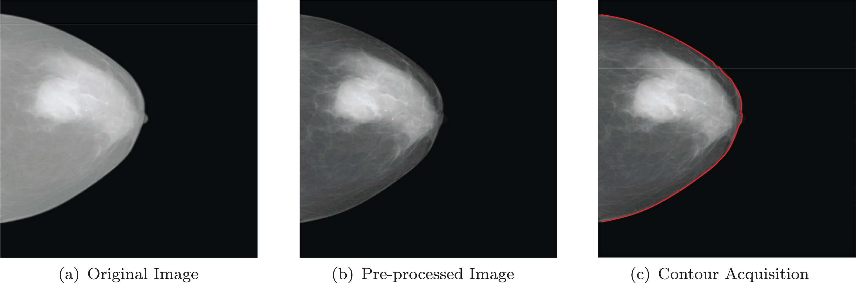
A Demonstration for image pre-processing and contour acquisition.

4.2.1.2. Contour acquisition.

After preprocessing, it is necessary to obtain the breast contour, which is the range of sub-region division. In this paper, the edge detection algorithm is used for contour acquisition. Since the information contained in edge pixels is obviously different from the information contained in background regions, and the edges have a first order differential maximum or minimum extremum because of a step change [9]. Canny [13] operator is a first-order differential multi-scale edge detector, which has better edge connectivity, so we use Canny operator for edge detection. The contour acquisition result is shown in Fig. 2 (b) and (c).

4.2.1.2. Sub-region division.

The main purpose of sub-region division is to divide the breast region into several sub-regions of equal size in order to extract the local features from each sub-region. And we will use a sliding window method to achieve this goal.

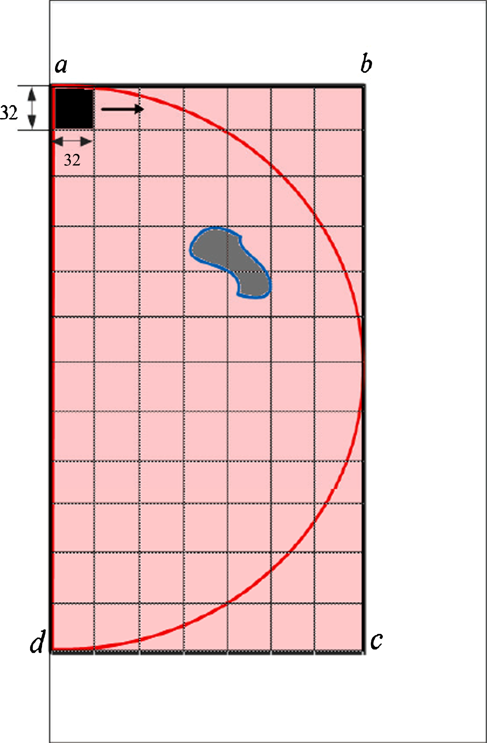
First, the sliding range is determined. Because the breast mass must be inside the breast area, we define a smallest rectangular area, which contains breast tissue, as the sliding range. The breast tissue contour is the boundary. (x₁, y₁), (x₂, y₂), (x₃, y₃) and (x₄, y₄), are the coordinates of the rectangular vertices, clockwise from the upper left corner to the bottom right corner.

Then, a 32 × 32 pixels square area is used as a sliding window to slide within this rectangular area. The window starts from the upper left corner, (x₁, y₁), in row-major order of rectangular area S, and the sliding step is always 32 pixels. When the four vertices are all outside the S region, the row is ended and the next line continues to slide. Sliding along the line in this way, and sliding stops until the last line of sliding window contains (x₃, y₃) and the four vertices are not all outside the S region. Fig. 3 shows a mammogram, where the red lines represent the boundary of the mammary gland; the gray ones represent the mass; the pink ones represent the rectangular region S; the four vertices of S are (x₁, y₁), (x₂, y₂), (x₃, y₃) and (x₄, y₄); the sliding window is represented by the 32 × 32 pixels black square area in the upper left corner; the step length is 32 pixels; the window slides in the direction of the arrow. Thus, the sub-region is the area of the sliding window at each step, and then, local density feature is extracted in these sub-regions.

Fig.3

An Example of the sliding window.

Here, we choose the square slide window and try the size of 2ⁿ × 2ⁿ during the experiment. And after comparison, we find 2⁵ × 2⁵ can get better results with less time and more clearly visual effects. Thus, we set 32 × 32 as the slide window size.

4.2.2 Density feature extraction

Since the density of the mass and the glandular tissue in mammograms is different, we can distinguish the mass region by local density feature of the sub-region. In mammograms, the mass region is usually dense and bright, but the normal tissue is usually sparse. And there are also some normal dense regions due to lots of fibro-glandular tissues (We call it dense region without mass.). In this section, we first analyze the density difference between these three regions. Then, we quantify the density feature based on these differences, and this density feature will be used to distinguish whether a sub-region is a mass region.

4.2.2.1 Density difference analysis

Tissues with Different density will present bright or dark, and gray-level histograms are also different. We crop different regions from the mammograms for analysis, as shown in Fig. 4. (a) shows the original image and the sub-regions of size 32 × 32, where (a-1) is the dense region without mass, (a-2) is the true mass region, (a-3) is the normal region (sparse region). The gray-level histograms are shown in (b), (c) and (d).

Fig.4

Density comparison of different sub-regions.

Comparing (d) with (b) and (c), the mean value of the sparse region histogram is obviously smaller than the dense region, and the sparse region histogram is more concentrated distribution. Then, comparing (b) and (c), we find that for the dense region, the mean value of mass region histogram is larger than dense region without mass. And the mass region histogram distributes more concentratedly. Since the histograms are different in mean value and skewness, density feature can be obtained by quantifying histograms.

4.2.2.2 Density feature description.

Because gray-level histograms of mass region, dense region without mass and sparse region are different, we describe mammary gland density feature based on the gray-level histograms. The density feature set includes density mean, density variance, density skewness, density kurtosis, gray-level density variance, gray-level density skewness, and gray-level density kurtosis [16], which are described as follows:

Density Mean: The Density mean is the average value of sub-regions, which reflects the distribution of the image density in each sub-region. The formula is Eq. (1). Where, L is the grey-level of pixels in a sub-region, z_i is the number of pixels of grey-level i and p (z_i) is the percentage that the number of pixels of grey-level i for the number of all pixels.

$d_{1} = \sum_{i = 0}^{L - 1} Z_{i} p (z_{i})$ (1)

Density Variance: The density variance describes the variation of the pixel density in the sub-region, which is used to extract the variance of the pixels in each sub-region. The formula is Eq. (2). Where, m is the gray-level mean of pixels in the sub-region.

$d_{2} = \sum_{i = 0}^{L - 1} (z_{i} - m)^{2} p (z_{i})$ (2)

Density Skewness: The density skewness describes the symmetry of the sub-region image density distribution, which is used to extract the skew of the pixels in each sub-region. The formula is Eq. (3).

$d_{3} = \frac{1}{d_{1}^{3 / 2}} \sum_{i = 0}^{L - 1} (z_{i} - m)^{3} p (z_{i})$ (3)

Density Kurtosis: The density kurtosis describes the relative flatness of the sub-region image density distribution, which is used to extract the kurtosis of the pixels in each sub-region. The formula is Eq. (4).

$d_{4} = \frac{1}{d_{1}^{2}} \sum_{i = 0}^{L - 1} (z_{i} - m)^{4} p (z_{i})$ (4)

Gray-level Density Variance: The gray-level density variance describes the variation of the gray density of the image in the sub-region, which is used to extract the variance of the gray-level density of each sub-region. The formula is Eq. (5). Where, the gray-level density of the pixels in the sub-region is calculated as the Eq. (6).

$d_{5} = \sum_{i = 0}^{L - 1} (z_{i} - p_{m})^{2} p (z_{i})$ (5)

$p_{m} = \frac{1}{L} \sum_{i = 0}^{L - 1} p (z_{i})$ (6)

Gray-level Density Skewness: The gray-level density skewness describes the symmetry of the gray-level density distribution of the image in the sub-region. It is used to extract the gray-level skew of the image in each sub-region. The formula is as follows Eq. (7).

$d_{6} = \frac{1}{d_{1}^{3 / 2}} \sum_{i = 0}^{L - 1} (z_{i} - p_{m})^{3} p (z_{i})$ (7)

Gray-level Density Kurtosis: The gray-level density kurtosis is the kurtosis of the gray-level density of the image in the sub-region. It is used to extract the kurtosis of the gray-level density of the image in each sub-region. The formula is Eq. (8).

$d_{7} = \frac{1}{d_{1}^{2}} \sum_{i = 0}^{L - 1} (z_{i} - p_{m})^{4} p (z_{i})$ (8)

4.2.3 Clustering based on US-ELM

After extracting the seven density features above, a US-ELM based clustering of density features is carried out. The two clustering groups are the regions of breast mass and non-mass. Because the regions of mass have higher average pixel values, we can use that to determine the tumor areas and detect them.

US-ELM algorithm for clustering is shown in Algorithm 1. The input is the local density feature vector D, and the output is the clustering result. Firstly, the Laplace transform matrix L is constructed from the input density feature vector D, and then the hidden layer node parameters (ω_i, b_i) are randomly generated to calculate the hidden layer node output matrix H. Next, comparing the number of hidden nodes and input nodes, the output weight β is calculated by different formulas. Fourthly, by using the Laplacian matrix L, the hidden layer output matrix H and the output weight β, the embedding matrix E is obtained. Finally, regarding each row in the matrix E as a point, the clustering result is obtained by the k-means method.

Algorithm 1 US-ELM algorithm
Input: The density feature vector: D ∈ R^N×n₀;
Output: The label vector of cluster index: y ∈ R^N×1.
1: Construct the graph Laplacian L from X.
2: Random output matrix of the hidden neurons H ∈ R^N×n_k.
3: ifn_h ≤ Nthen
4: Calculate output weight β by $min_{β \in R^{n_{h} \times n_{0}}} ∥ β ∥^{2} + λ Tr (β^{T} H^{T} LH β)$ .
5: else
6: Calculate output weight β by (I₀ + lH^TLH) v = γH^THv.
7: end if
8: Calculate the embedding matrix: E = Hβ.
9: Treat each row of E as a point, and cluster the N points into K clusters using the
k-means algorithm. Let y be the label vector of cluster index for all the points.
10: returny.

4.3 ELM based diagnosis using fused features with density

After finishing breast mass detection by sub-region density clustering, we also propose a breast mass diagnosis method based on ELM using fused features with density (BMDx). Especially, since we have already got the mass region by detection, diagnosis is performed on the whole breast mass region. Firstly, morphology, texture and density features are extracted from the whole mass region, and a fusion feature model (fused features with density) is built. Then, the model is optimized by feature selection. Finally, ELM is used to classify benign or malignant mass.

4.3.1 Fusion feature modeling

According to the radiologists’ clinical experience, in addition to the density of the tumor, the geometry and texture features are also considered. The geometry features, such as the roughness, size and shape of the mass, is important to distinguish the mass quality. Texture is a common visual phenomenon, which can reflect the color pattern, surface roughness and the gray-level direction, so it can be used as an effective feature to classify masses. Therefore, the feature model considers the density features, geometry features and texture features together. The feature vectors are shown in Eq. (9).

$F = [F_{1}, F_{2}, F_{3}]$ (9)

The feature vectors of density, geometry and texture features are shown in Eqs. (10, 11, 12), respectively. Furthermore, the 7 global density features, 8 geometry features, and 11 texture features are described in detail below.

$F_{1} = [d_{1}, d_{2}, d_{3}, d_{4}, d_{5}, d_{6}, d_{7}]$ (10)

$F_{2} = [g_{1}, g_{2}, g_{3}, g_{4}, g_{5}, g_{6}, g_{7}, g_{8}]$ (11)

$F_{3} = [t_{1}, t_{2}, t_{3}, t_{4}, t_{5}, t_{6}, t_{7}, t_{8}, t_{9}, t_{10}, t_{11}]$ (12)

4.3.1.1 Density features.

In Eq. (10), the density features of the 7 sub-regions d₁, d₂, d₃, d₄, d₅, d₆, d₇ of the mass are the density mean, density variance, density skewness, density kurtosis, gray-level density variance, gray-level density skewness and gray-level density kurtosis [16]. The above features are shown in Table 1, where the meaning of each parameter is as shown in Section 4.2.2.

Table 1
Density features

Name Features expression

Density mean $d_{1} = \sum_{i = 0}^{L - 1} Z_{i} p (z_{i})$

Density variance $d_{2} = \sum_{i = 0}^{L - 1} (z_{i} - m)^{2} p (z_{i})$

Density skewness $d_{3} = \frac{1}{d_{1}^{3 / 2}} \sum_{i = 0}^{L - 1} (z_{i} - m)^{3} p (z_{i})$

Density kurtosis $d_{4} = \frac{1}{d_{1}^{2}} \sum_{i = 0}^{L - 1} (z_{i} - m)^{4} p (z_{i})$

Gray-level density variance $d_{5} = \sum_{i = 0}^{L - 1} (z_{i} - p_{m})^{2} p (z_{i})$

Gray-level density skewness $d_{6} = \frac{1}{d_{1}^{3 / 2}} \sum_{i = 0}^{L - 1} (z_{i} - p_{m})^{3} p (z_{i})$

Gray-level density kurtosis $d_{7} = \frac{1}{d_{1}^{2}} \sum_{i = 0}^{L - 1} (z_{i} - p_{m})^{4} p (z_{i})$

Name	Features expression
Density mean	$d_{1} = \sum_{i = 0}^{L - 1} Z_{i} p (z_{i})$
Density variance	$d_{2} = \sum_{i = 0}^{L - 1} (z_{i} - m)^{2} p (z_{i})$
Density skewness	$d_{3} = \frac{1}{d_{1}^{3 / 2}} \sum_{i = 0}^{L - 1} (z_{i} - m)^{3} p (z_{i})$
Density kurtosis	$d_{4} = \frac{1}{d_{1}^{2}} \sum_{i = 0}^{L - 1} (z_{i} - m)^{4} p (z_{i})$
Gray-level density variance	$d_{5} = \sum_{i = 0}^{L - 1} (z_{i} - p_{m})^{2} p (z_{i})$
Gray-level density skewness	$d_{6} = \frac{1}{d_{1}^{3 / 2}} \sum_{i = 0}^{L - 1} (z_{i} - p_{m})^{3} p (z_{i})$
Gray-level density kurtosis	$d_{7} = \frac{1}{d_{1}^{2}} \sum_{i = 0}^{L - 1} (z_{i} - p_{m})^{4} p (z_{i})$

4.3.1.2 Geometry features.

In Eq. (11), g₁, g₂, g₃, g₄, g₅, g₆, g₇, g₈ are the 8 geometry features, which are the roundness, entropy of standardized radius, variance of standardized radius, ratio of area, G-roughness, circularity, length-width ratio and squareness [27]. The above features are shown in Table 2. A is the area of mass and P is the girth of edge; p_k is the probability of standardized histogram; N is the number of edge points; d_i is the average standardized radius of edge points; μ_R is the average distance from the center of gravity to the boundary point. σ_R is the mean square deviation distance from the center of gravity to the boundary point; H_ROI and W_ROI are the length and width of the circumscribed rectangle of the mass; A_MER is the smallest rectangular area surrounding a mass.

Table 2
Geometry features

Name Features expression

Roundness $g_{1} = \frac{p^{2}}{A}$

Entropy of standardized radius $g_{2} = - \sum_{k = 1}^{100} p_{k} (log (p_{k}))$

Variance of standardized radius $g_{3} = \sqrt{\frac{1}{N - 1} \sum_{t = 1}^{N} (d_{i} - d_{avg})^{2}}$

Ratio of area $g_{4} = \frac{1}{d_{avg} N} \sum_{i = 1}^{N} (d_{i} - d_{avg})$

G-roughness $g_{5} = \frac{1}{N} \sum_{i = 1}^{N} | d_{i} - d_{i + 1} |$

Circularity $g_{6} = \frac{μ_{R}}{σ_{R}}$

Length-width ratio $g_{7} = \frac{H_{ROI}}{W_{ROI}}$

Squareness $g_{8} = \frac{A}{A_{MER}}$

Name	Features expression
Roundness	$g_{1} = \frac{p^{2}}{A}$
Entropy of standardized radius	$g_{2} = - \sum_{k = 1}^{100} p_{k} (log (p_{k}))$
Variance of standardized radius	$g_{3} = \sqrt{\frac{1}{N - 1} \sum_{t = 1}^{N} (d_{i} - d_{avg})^{2}}$
Ratio of area	$g_{4} = \frac{1}{d_{avg} N} \sum_{i = 1}^{N} (d_{i} - d_{avg})$
G-roughness	$g_{5} = \frac{1}{N} \sum_{i = 1}^{N} \| d_{i} - d_{i + 1} \|$
Circularity	$g_{6} = \frac{μ_{R}}{σ_{R}}$
Length-width ratio	$g_{7} = \frac{H_{ROI}}{W_{ROI}}$
Squareness	$g_{8} = \frac{A}{A_{MER}}$

4.3.1.3. Texture features.

In Eq. (12), t₁, t₂, t₃, t₄, t₅ are the 5 texture features based on Gray-level Co-occurrence Matrix (GLCM) [16], which are inverse difference moment, entropy, energy, correlation coefficient, G-contrast [26]. And t₆, t₇, t₈, t₉, t₁₀, t₁₁ are the 6 texture features proposed by Tamura et al. [23], including coarseness, contrast (T-contrast), directionality, line-likeness, regularity and T-roughness. The above features are shown in Table 3. P (i, j) is the element of row i and column j of GLCM; μ_x, μ_y, δ_x, δ_y are the average and variance of rows and columns of P; m and n are the length and width of the image and S_best (i, j) is the best window size; μ is the statistical mean of whole image pixel and σ is the statistical variance of whole image pixel; n_p is the number of peaks in the histogram, p is the peak in the histogram H_D, ω_p is the range of quantization values that p contains and φ_p is the quantization value in the maximum histogram value of ω_p; P_Dd is the distance point of local co-occurrence matrix of n × n; r is a normalization factor; σ_x is the standard deviation of t_x; t₆ is the coarseness and t₇ is the T-contrast.

Table 3
Texture features

Name Features expression

Inverse difference moment $t_{1} = \sum \frac{P (i, j)}{1 + (i - j)^{2}}$

Entropy t₂ = ∑P (i, j) × [- ln P (i, j)]

Energy t₃ = ∑P² (i, j)

Correlated coefficient $t_{4} = \sum \frac{P (i, j) (i - μ_{x}) (j - μ_{y})}{δ_{x} δ_{y}}$

G-contrast t₅ = (i - j) ²P (i, j)

Coarseness $t_{6} = \frac{1}{m \times n} \sum_{i - 1}^{m} \sum_{j - 1}^{n} S_{best} (i, j)$

T-contrast $t_{7} = \frac{σ}{\sqrt[4]{(μ^{4} / σ^{4})^{4}}}$

Directionality $t_{8} = \sum_{p}^{n_{p}} \sum_{φ \in ω_{p}} (φ - φ_{p})^{2} H_{D} (φ)$

Line-likeness $t_{9} = \frac{\sum_{i}^{n} \sum_{j}^{n} P_{Dd} (i, j) cos [(i - j) 2 π / n]}{\sum_{i}^{n} \sum_{j}^{n} P_{Dd} (i, j)}$

Regularity t₁₀ = 1 - r (σ₆ + σ₇ + σ₈ + σ₉)

T-roughness t₁₁ = t₆ + t₇

Name	Features expression
Inverse difference moment	$t_{1} = \sum \frac{P (i, j)}{1 + (i - j)^{2}}$
Entropy	t₂ = ∑P (i, j) × [- ln P (i, j)]
Energy	t₃ = ∑P² (i, j)
Correlated coefficient	$t_{4} = \sum \frac{P (i, j) (i - μ_{x}) (j - μ_{y})}{δ_{x} δ_{y}}$
G-contrast	t₅ = (i - j) ²P (i, j)
Coarseness	$t_{6} = \frac{1}{m \times n} \sum_{i - 1}^{m} \sum_{j - 1}^{n} S_{best} (i, j)$
T-contrast	$t_{7} = \frac{σ}{\sqrt[4]{(μ^{4} / σ^{4})^{4}}}$
Directionality	$t_{8} = \sum_{p}^{n_{p}} \sum_{φ \in ω_{p}} (φ - φ_{p})^{2} H_{D} (φ)$
Line-likeness	$t_{9} = \frac{\sum_{i}^{n} \sum_{j}^{n} P_{Dd} (i, j) cos [(i - j) 2 π / n]}{\sum_{i}^{n} \sum_{j}^{n} P_{Dd} (i, j)}$
Regularity	t₁₀ = 1 - r (σ₆ + σ₇ + σ₈ + σ₉)
T-roughness	t₁₁ = t₆ + t₇

4.3.2 Feature selection optimization

There are 26 features in the fusion feature model. Among these features, there may be a strong correlation, which can affect the machine learning ability and reduce the accuracy of the diagnosis. Therefore, it is necessary to optimize the fusion feature model. Genetic Algorithm Selection (GAS) [27] is a stochastic search algorithm that mimics the natural selection and genetic process to find the most adaptive individual, ie finding the optimal diagnostic accuracy of the feature model. GAS [15] has the characteristics of parallel processing data, wide application and easy implementation, so this algorithm is used to select the existing features and optimize. The GAS algorithm is shown in Algorithm 2.

4.3.3 Diagnosis of breast mass

After optimization, the feature model is used to diagnose breast masses. ELM includes training and diagnosis processes. During the training process, the input includes the fusion feature of the mass and the pathological diagnosis result. In the diagnosis process, the input is the fusion feature of the mass to be diagnosed.

Algorithm 2 Genetic Algorithm Selection
Input: Original feature vector model, threshold S, genetic algebra G;
Output: New feature vector model F.
1: Random a feature vector model containing N features and calculate the individual
fitness of initial population.
2: fori = 1 to Gdo
3: forj = 1 to Gdo
4: if individual fitness > Sthen
5: The feature as the parent generation to the younger generation.
6: end if
7: end for
8: end for
9: The parent generation with a higher individual fitness generates new off spring.
10: Obtain the optimized feature vector model and the detection accuracy.
11: returnF.

4.3.3.1 Feature extraction.

Before the training and diagnosis, the fusion feature F is extracted from mammograms. The feature extraction algorithm is shown in Algorithm 3. This algorithm is performed on all A images in the image dataset, until the optimized fusion feature F is extracted separately, which is used for subsequent training and diagnosis of ELM.

Algorithm 3 Feature Extraction Algorithm
Input:A:the number of image set;
Output:F: the optimized fusion feature F of mass in each mammogram.
1: fori = 1 to A
2: Read image after segmenting the mass.
3: end for
4: Get density features of mass areas.
5: Get geometry features of mass areas.
6: Get texture features of mass areas.
7: Get fusion features of mass areas.
8: returnF.

4.3.3.2 ELM training.

The optimized fusion feature F of the mass area in T training images are obtained by Algorithm 3. Pathological diagnosis result P and optimized fusion feature F are used as the training data, and then, ELM training process can be carried out. In addition to the training data, the ELM training process also needs the hidden layer node number L, in order to randomly generate hidden layer node parameters (ω_i, b_i). The ELM training algorithm is shown in Algorithm 4.

Algorithm 4 ELM Training Algorithm
Input:T:the number of training image set, P: pathological diagnosis result, L: the
number of hidden layer node;
Output:ω, b, β: 3 parameters of ELM.
1: fori = 1 to T
2: Transfer the algorithm 3 to obtain F.
3: end for
4: fori = 1 to Ldo
5: Randomly generate hidden node parameters (ω_i, b_i).
6: end for
7: Calculate the hidden layer output matrix H.
8: Calculate the output weight vector β = H^TP.
9: returnω, b, β.

4.3.3.3 ELM diagnosis.

During the ELM training process, the parameters ω, b and β of the classifier are first obtained. Then, the diagnosis of breast mass is carried out to determine the benign and malignant cases. D images are operated by Algorithm 3, in order to obtain the optimized fusion feature F of the masses as the input data of the ELM diagnosis. ELM Diagnosis Algorithm is shown in Algorithm 5.

Algorithm 5 ELM Diagnosis Algorithm
Input:D: the number of images that to be diagnosed, L: the number of hidden
layer node, ω, b, β: parameters of ELM;
Output:R: diagnostic result.
1: fori = 1 to D
2: Transfer the algorithm 3 to obtain F.
3: end for
4: Calculate the hidden layer output matrix H use F, ω and b.
5: Get diagnostic result R = Hβ.
6: returnR.

5 Experiments and Results

In this paper, we validate the effectiveness of the methods including the detection method based on sub-region density clustering of US-ELM (BMDe) and the diagnosis method based on the ELM using a density feature fusion (BMDx) on a real dataset. In this chapter, the experimental setting is first introduced. Then, the experimental scheme and parameter setting are introduced. Then, the evaluation methods of the experimental results are described. Finally, the experimental results of each experiment are listed and analysis.

5.1 Detection scheme and parameters

In the experiment of breast mass detection, the method BMDe proposed in this paper is used. Another 3 common methods are used for comparison, including Watershed Algorithm (WA) [6], Multi-thresholds Segmentation Algorithm (MSA) [10] and Region Grow Algorithm (RGA) [30]. In order to compare clearly, BMDe and another 3 methods are used to segment the same image, and the manually segmentation from radiologists are used as the standard.

Also, US-ELM is used during detection, and parameters include the hidden layer node number L and cluster number k. The number of hidden layer nodes is set to 1000 by pre-tests, and the activation function S selects the sigmoid function. Since we use US-ELM to cluster into 2 classes based on local density feature, k value is set to 2.

5.2 Detection evaluation indicators

In the detection of breast masses, we use Precision and Recall to evaluate the accuracy. Also, in order to compare the segmentation methods mentioned in Section 5.1, we choose another 5 indicators, including Misclassified Error (ME), Area Overlap Metric (AOM), Area Over-segmentation Measure (AVM), Area Under-segmentation Measure (AUM) and Combination Measure (CM).

Detection evaluation indicators and the formulas are shown in Table 4, where TP (True Positive) is the number of masses which are successfully detection; FN (False Negative) is the number of masses which are not successfully detection; FP (False Positive) is the number of non-masses which are detected as the masses; S_A is the area of target region segmented by the algorithm; S_B is the area of the exact segmentation region (In this experiment, S_B is the area of the mass region marked by experienced radiologists); α, β, λ are weights. Because CM is overall consideration of AOM, AVM and AUM, α, β, and λ are set as equivalent and the values of them are 1/3 in this paper. Especially for BMDe method, the mass is obtained by clustering the windows. And then, we smooth the mass area according to convex hull [3], and the outer points of sub-region clustering results are connected to form a convex polygon.

Table 4
Evaluation indices of detection

Evaluation indices Formula expression

Precision $\frac{TP}{(TP + FP)}$

Recall $\frac{TP}{(TP + FN)}$

ME $\frac{Area {S_{A} \cup S_{B}} - Area {S_{A} \cap S_{B}}}{Area {S_{B}}}$

AOM $\frac{Area {S_{A}} \cap Area {S_{B}}}{Area {S_{A}} \cup Area {S_{B}}}$

AVM $\frac{Area {S_{A}} - Area {S_{B}}}{Area {S_{A}}}$

AUM $\frac{Area {S_{B}} - Area {S_{A}}}{Area {S_{B}}}$

CM αAOM + β (1 - AUM) + λ (1 - AVM)

Evaluation indices	Formula expression
Precision	$\frac{TP}{(TP + FP)}$
Recall	$\frac{TP}{(TP + FN)}$
ME	$\frac{Area {S_{A} \cup S_{B}} - Area {S_{A} \cap S_{B}}}{Area {S_{B}}}$
AOM	$\frac{Area {S_{A}} \cap Area {S_{B}}}{Area {S_{A}} \cup Area {S_{B}}}$
AVM	$\frac{Area {S_{A}} - Area {S_{B}}}{Area {S_{A}}}$
AUM	$\frac{Area {S_{B}} - Area {S_{A}}}{Area {S_{B}}}$
CM	αAOM + β (1 - AUM) + λ (1 - AVM)

5.3 Diagnosis schemes and parameters

In the diagnosis of breast masses, the feature models and classifiers are validated, respectively. In the verification of the feature models, the results of mass diagnosis under five feature vector models are compared, respectively. The five feature vector models are: 1. geometry features + texture features (GT) model; 2. geometry features + density features (GD) model; 3. texture features + density features (TD) model; 4. geometry features + texture features + density features (GTD) model; 5. (GTD*) model, which is an GAS optimized GTD model. In the verification of the classifier, the results of mass diagnosis based on three classifiers are compared, respectively. The three classifiers are: 1. BP, 2. SVM, 3. ELM. The specific experimental scheme and simplified identification are shown in Table 5.

Table 5
Diagnosis experimental schemes

Classifiers GT GD TD GTD GTD*

BP GT-BP GD-BP TD-BP GTD-BP GTD-BP

SVM GT-SVM GD-SVM TD-SVM GTD-SVM GTD-SVM

ELM GT-ELM GD-ELM TD-ELM GTD-ELM GTD*-ELM

Classifiers	GT	GD	TD	GTD	GTD*
BP	GT-BP	GD-BP	TD-BP	GTD-BP	GTD*-BP
SVM	GT-SVM	GD-SVM	TD-SVM	GTD-SVM	GTD*-SVM
ELM	GT-ELM	GD-ELM	TD-ELM	GTD-ELM	GTD*-ELM

In the diagnosis of breast mass, five feature vector models are tested using BP, SVM and ELM classifiers. The parameters involved in the genetic selection algorithm used in the feature selection optimization process have the initial number of features N, the genetic algebra G and the individual fitness threshold S. In the experiment, N is 26, G is 100 and S is 80% based on experience. In the case of mass diagnosis based on BP, the parameters involved are the activation function S, the error tolerance limit e and the hidden layer node number L. In the experiment, the sigmoid function is chosen as the activation function S, and the error tolerance limit e is set to 1e-4. Under the five different feature models, the numbers of hidden nodes are 10, 11, 13, 12 and 11. In the experiment based on SVM, there are three parameters, including kernel function R, the penalty coefficient c and the kernel function parameter g. Furthermore, the RBF is selected as the R, c is set to 0.5, and g is set to 0.0206 by our pre-tests. In the case of mass-based diagnosis experiments based on ELM, the parameters involved are the activation function S, and the hidden layer node number L. In the experiment, the selected activation function is sigmoid, and the number of hidden nodes is set to 1000 by pre-tests. The choose of kernel functions in SVM have an enormous impact on the classification performance. RBF kernel function based SVM is considered classical, so we directly use it in our method.

5.4 Diagnosis evaluation indicators

Accuracy, Sensitivity, Specificity, True Positive Ratio (TP Ratio), True Negative Ratio (TN Ratio) and Area Under ROC (AUC) are used to evaluate diagnosis results. Diagnosis evaluation indicators and formulas are shown in Table 6. In order to get universal results, cross-validation [5] is used. In the experiment, we use 8-fold cross-validation to get the evaluation indicators. Among these 6 indicators, the larger the value, the more accurate the diagnosis is. In Table 6, TP (True Positive) is the number of malignant masses that can be accurately diagnosed; TN (True Negative) is the number of benign masses that can be accurately diagnosed; FN (False Negative) is the number of malignant masses that cannot be accurately diagnosed; FP (False Positive) is the number of benign masses that cannot be accurately diagnosed; x_i is the abscissa value of i in ROC; y_i is the ordinate value of i in ROC.

Table 6
Evaluation indices of diagnosis

Evaluation indices Formula expression

Accuracy (TP + TN)/(TP + TN + FP + FN)

Sensitivity TP/(TP + FN)

Specificity TN/(TN + FP)

TP Ratio TP/(TP + FP)

TN Ratio TN/(TN + FN)

AUC $AUC = \sum_{i = 1}^{N} (y_{i} + y_{i - 1}) (x_{i - 1} - x_{i}) / 2$

Evaluation indices	Formula expression
Accuracy	(TP + TN)/(TP + TN + FP + FN)
Sensitivity	TP/(TP + FN)
Specificity	TN/(TN + FP)
TP Ratio	TP/(TP + FP)
TN Ratio	TN/(TN + FN)
AUC	$AUC = \sum_{i = 1}^{N} (y_{i} + y_{i - 1}) (x_{i - 1} - x_{i}) / 2$

5.5 Result analysis

In this section, our proposed methods, BMDe and BMDx, are compared with other common methods to analyze the experimental results. BMDe is compared to three common segmentation method, including WA, MSA and RGA. And BMDx is compared using different kinds of classifiers and feature models. Especially, we use 246 images for diagnosis (There are 246 images with masses in our dataset.).

5.5.1 Analysis of detection results

During detection, the BMDe proposed in this paper is compared with another 3 common segmentation methods. Fig. 5 is demonstration of different segmentation methods. A further comparison of these 4 methods is shown in Table 7 and Fig. 6 based on Detection Evaluation Indicators. The results show that BMDe method has higher precision and recall, and ME value is smaller, and CM value is larger. Thus, BMDe has a better performance when detection.

Fig.5

Demonstration of different segmentation methods.

Table 7

Evaluation indicators of detection

	Precision	Recall	ME	AOM	AVM	AUM	CM
BMDe	0.9184	0.9146	0.2196	0.9122	0.0787	0.0752	0.9194
WA	0.8926	0.8710	0.3090	0.8706	0.1269	0.1025	0.8804
MSA	0.8785	0.8893	0.3827	0.8673	0.1554	0.2697	0.8141
RGA	0.9016	0.8907	0.4019	0.8231	0.0226	0.03853	0.8051

Fig.6

Evaluation indicators of detection.

5.5.2 Analysis of diagnosis results

According to the Diagnosis experimental schemes in Table 5, the accuracy, sensitivity, specificity, TP Ratio, TN Ratio and AUC are analyzed based on 3 kinds of classifiers and 5 kinds of feature models. The results are shown in Table 8.

The results based on BP, SVM and ELM, are shown in Fig. 7, 8 and 9. The results show that, whatever classifiers we use, the optimized feature model (GTD*) can get better results.

For 5 feature models of GT, GD, TD, GTD and GTD*, the ROC results are shown in Fig. 10– 14. The results show that, whatever feature models we use, ELM classifier can get better results.

Therefore, the optimized fusion feature model based on ELM classifier is optimal in breast mass diagnosis.

Table 8
Evaluation indicators of diagnosis

Category Accuracy Sensitivity Specificity TP Ratio TN Ratio AUC

GT BP 0.730 0.713 0.718 0.784 0.603 0.710

SVM 0.812 0.800 0.793 0.877 0.694 0.798

ELM 0.833 0.821 0.810 0.903 0.719 0.824

GD BP 0.744 0.761 0.741 0.802 0.644 0.738

SVM 0.827 0.848 0.819 0.894 0.729 0.818

ELM 0.851 0.866 0.842 0.917 0.753 0.848

TD BP 0.753 0.771 0.734 0.818 0.725 0.767

SVM 0.838 0.859 0.814 0.901 0.812 0.849

ELM 0.864 0.882 0.835 0.925 0.830 0.862

GTD BP 0.789 0.814 0.776 0.840 0.747 0.798

SVM 0.871 0.903 0.847 0.929 0.838 0.871

ELM 0.895 0.926 0.873 0.948 0.846 0.881

GTD* BP 0.802 0.826 0.805 0.847 0.771 0.807

SVM 0.889 0.915 0.878 0.931 0.850 0.919

ELM 0.911 0.933 0.901 0.952 0.869 0.938

Category	Accuracy	Sensitivity	Specificity	TP Ratio	TN Ratio	AUC
GT	BP	0.730	0.713	0.718	0.784	0.603	0.710
SVM	0.812	0.800	0.793	0.877	0.694	0.798
ELM	0.833	0.821	0.810	0.903	0.719	0.824
GD	BP	0.744	0.761	0.741	0.802	0.644	0.738
SVM	0.827	0.848	0.819	0.894	0.729	0.818
ELM	0.851	0.866	0.842	0.917	0.753	0.848
TD	BP	0.753	0.771	0.734	0.818	0.725	0.767
SVM	0.838	0.859	0.814	0.901	0.812	0.849
ELM	0.864	0.882	0.835	0.925	0.830	0.862
GTD	BP	0.789	0.814	0.776	0.840	0.747	0.798
SVM	0.871	0.903	0.847	0.929	0.838	0.871
ELM	0.895	0.926	0.873	0.948	0.846	0.881
GTD*	BP	0.802	0.826	0.805	0.847	0.771	0.807
SVM	0.889	0.915	0.878	0.931	0.850	0.919
ELM	0.911	0.933	0.901	0.952	0.869	0.938

Fig.7

Comparison of evaluation indexes based on BP.

Fig.8

Comparison of evaluation indexes based on SVM.

Fig.9

Comparison of evaluation indexes based on ELM.

Fig.10

ROC result of GT feature model.

Fig.11

ROC result of GD feature model.

Fig.12

ROC result of TD feature model.

Fig.13

ROC result of GTD feature model.

Fig.14

ROC result of GTD* feature model.

6 Conclusion

In order to improve the accuracy of computer-aided breast mass detection and diagnosis, this paper proposes a method of computer-aided breast mass detection and diagnosis. The main contributions of our work are as follows:

A mass detection method based on US-ELM using sub-region density clustering is proposed, simply as BMDe. This method can reach 0.9184 precision in mass detection.

A mass diagnosis method based on ELM using fused features with density is proposed, simply as BMDe. This method can reach 0.911 accuracy in mass diagnosis.

These two methods are operated on the real mammograms from Northeast China. We compare them with other common methods, and the results show that the proposed method, BMDe and BMDe, have obvious advantages in multiple indicators.

In this paper, local density feature is used in breast mass detection, and global optimized fusion feature model is used to diagnose benign or malignant breast masses. First, computer-aided detection of breast masses is achieved using sub-region density clustering based on US-ELM. Then, fused feature with density is used to realize the computer-aided diagnosis based on ELM. Finally, the methods of breast mass detection and diagnosis are performed on the real mammograms from Northeast China. The experiments show that, comparing with Watershed Algorithm, Multi-thresholds Segmentation Algorithm and Region Grow Algorithm, BMDe proposed has obvious advantages in precision and other indicators. And comparing with double fusion feature model (GT, GD, TD) and the three fusion feature model (GTD), the optimized three fusion feature model (GTD*) has obvious advantages in the mass diagnosis. Comparing to SVM and BP, ELM classifier performs better.

Disclosure statement

The work described has not been published previously in any form. All authors declare that they have no competing interests. There are no financial or personal relationships with other people or organisations that could inappropriately influence our work.

Funding

This research was partially supported by the National Natural Science Foundation of China (Nos. 61472069, 61402089, and U1401256), the China Postdoctoral Science Foundation (No. 2018M641705), the Fundamental Research Funds for the Central Universities (Nos. N161602003, N161904001, and N160601001), the Fund of Acoustics Science and Technology Laboratory of Harbin Engineering University, and the Open Program of Neusoft Research of Intelligent Healthcare Technology, Co. Ltd. (No. NRIHTOP1802).

References

Anitha and

J.D.

Peter , A wavelet based morphological mass detection and classification in mammograms, In: International Conference on Machine Vision and Image Processing (2012), pp. 25–28.

G.M.

Brake and

Karssemeijer , Segmentation of suspicious densities in digital mammograms, Medical Physics 28(2) (2001), 259–266.

T.M.

Chan , Optimal output-sensitive convex hull algorithms in two and three dimensions, Discrete and Computational Geometry 4(16) (1996), 361–368.

Chang ,

Hsiao and

Hsieh , An adaptive median filter for image denoising, In: Second International Symposium on Intelligent Information Technology Application (2008), pp. 346–350.

Dai , A competitive ensemble pruning approach based on cross-validation technique, Knowledge-Based Systems 37(2) (2013), 394–414.

R.B.

Dubey ,

Hanmandlu and

S.K.

Gupta , A comparison of two methods for the segmentation of masses in the digital mammograms, Computerized Medical Imaging and Graphics the Official Journal of the Computerized Medical Imaging Society 34(3) (2010), 185–191.

Z.G.

Fu ,

M.F.

Qi and

Jing , Regression forecast of main steam flow based on mean impact value and support vector regression, In: Power and Energy Engineering Conference (APPEEC), 2012 Asia-Pacific. IEEE. (2012), pp. 1–5.

Guo ,

Shao and

V.F.

Ruiz , Characterization and classification of tumor lesions using computerized fractal-based texture analysis and support vector machines in digital mammograms, International Journal of Computer Assisted Radiology and Surgery 4(1) (2009), 11.

W.Y.

Hsu , Improved watershed transform for tumor segmentation: Application to mammogram image compression, Expert Systems with Applications 39(4) (2012), 3950–3955.

10.

Hu ,

Gao and

Li , Detection of suspicious lesions by adaptive thresholding based on multiresolution analysis in mammograms, IEEE Transactions on Instrumentation and Measurement 60(2) (2011), 462–472.

11.

Huang ,

Song ,

J.N.

Gupta and

Wu , Semi-supervised and unsupervised extreme learning machines, IEEE Transactions on Cybernetics 44(12) (2017), 2405–2417.

12.

G.B.

Huang ,

Q.Y.

Zhu and

C.K.

Siew , Extreme learning machine: Theory and applications, Neurocomputing 70(1-3) (2006), 489–501.

13.

J , A computational approach to edge detection, IEEE transactions on pattern analysis and machine intelligence 8(6) (1986), 679–698.

14.

Leonardis ,

Bischof and

Pinz , Computer Vision - ECCV 2006:9th European Conference on Computer Vision, Graz, Austria, May 7-13, 2006, Proceedings, Part II (Lecture Notes in Computer Science). Springer-Verlag New York, Inc., Austria (2006).

15.

Li and

Zeng , Feature selection method with multi-population agent genetic algorithm, In: Advances in NeuroInformation Processing, International Conference, ICONIP 2008, Auckland, New Zealand, November 25-28, 2008, Revised Selected Papers. (2008), pp. 493–500.

16.

Liu ,

Wang and

He , Breast density classification using histogram moments of multiple resolution mammograms, In: International Conference on Biomedical Engineering and Informatics (2010), pp. 146–149.

17.

Liu ,

Zhou and

Tang , A benign and malignant mass classification algorithm based on an improved level set segmentation and texture feature analysis, In: International Conference on Bioinformatics and Biomedical Engineering (2010), pp. 1–4.

18.

Liu and

Y.F.

Zheng , Fss-fs: A novel feature selection method for support vector machines, Pattern Recognition 39(7) (2006), 1333–1345.

19.

M.D.

Luca ,

Grossi ,

Borroni ,

Zimmermann ,

Marcello ,

Colciaghi ,

Gardoni ,

Intraligi ,

Padovani and

Buscema , Artificial neural networks allow the use of simultaneous measurements of alzheimer disease markers for early detection of the disease, Journal of Translational Medicine 3(1) (2005), 1–7.

20.

M.J.

Morton ,

D.H.

Whaley ,

K.R.

Brandt and

K.K.

Amrami , Screening mammograms: Interpretation with computer-aided detection-prospective evaluation, Radiology 239(2) (2006), 375–383.

21.

R.L.

Siegel ,

K.D.

Miller ,

S.A.

Fedewa ,

D.J.

Ahnen ,

Rgs ,

Barzi and

Jemal , Colorectal cancer statistics, 2017. CaA Cancer Journal for Clinicians 67(3) (2017), 177–193.

22.

V.P.

Singh ,

Srivastava and

Srivastava , Automated and effective content-based image retrieval for digital mammography, Journal of X-ray science and technology 26(1) (2018), 29–49.

23.

Tamura ,

Mori and

Yamawaki , Textural features corresponding to visual perception, IEEE Transactions on Systems Man and Cybernetics 8(6) (1978), 460–473.

24.

Wang ,

Chen and

Zhang , Image enhancement based on equal area dualistic sub-image histogram equalization method, IEEE Transactions on Consumer Electronics 45(1) (1999), 68–75.

25.

Wang ,

Aghaei ,

Zarafshani ,

Qiu ,

Qian and

Zheng , Computer-aided classification of mammographic masses using visually sensitive image features, Journal of X-ray Science and technology 25(1) (2017), 171–186.

26.

Wang ,

Qu ,

Yu x and

Kang , Breast tumor detection in double views mammography based on extreme learning machine, Neural Computing and Applications 27(1) (2016), 227–240.

27.

Wang ,

Yu ,

Kang ,

Zhao and

Qu , Breast tumor detection in digital mammography based on extreme learning machine, Neurocomputing 128(5) (2014), 175–184.

28.

Wirn ,

Hggstrm ,

Ulmer ,

Manjer ,

Bjrge ,

Nagel ,

Johansen ,

Hallmans ,

Engeland and

Concin , Pooled cohort study on height and risk of cancer and cancer death, Cancer Causes and Control 25(2) (2014), 151–159.

29.

R.W.

Woods ,

G.S.

Sisney ,

L.R.

Salkowski ,

Shinki ,

Lin and

E.S.

Burnside , The mammographic density of a mass is a significant predictor of breast cancer, International Journal of Medical Radiology 258(2) (2011), 417–425.

30.

Zhang and

S.W.

Foo , Computer aided detection of breast masses from digitized mammograms, International Congress 1281(6) (2006), 1955–1961.

31.

Zheng ,

Tan ,

Piyarajan and

David , Association between computed tissue density asymmetry in bilateral mammograms and near-term breast cancer risk, Breast Journal 20(3) (2014), 249–257.

Breast mass detection and diagnosis using fused features with density

Abstract

BACKGROUND:

METHODS:

RESULTS:

CONCLUSIONS:

Keywords

1. Introduction

2 Background

3 Material

4 Methods

4.1 Mass detection and diagnosis framework

4.2.1 Sub-region division

4.2.1.1. Image preprocessing.

4.2.1.2. Sub-region division.

4.2.2.1 Density difference analysis

4.3 ELM based diagnosis using fused features with density

4.3.1 Fusion feature modeling

4.3.3 Diagnosis of breast mass

4.3.3.1 Feature extraction.

4.3.3.2 ELM training.

4.3.3.3 ELM diagnosis.

5 Experiments and Results

5.1 Detection scheme and parameters

5.2 Detection evaluation indicators

Table 5 Diagnosis experimental schemes Classifiers GT GD TD GTD GTD* BP GT-BP GD-BP TD-BP GTD-BP GTD*-BP SVM GT-SVM GD-SVM TD-SVM GTD-SVM GTD*-SVM ELM GT-ELM GD-ELM TD-ELM GTD-ELM GTD*-ELM

Table 6 Evaluation indices of diagnosis Evaluation indices Formula expression Accuracy (TP + TN)/(TP + TN + FP + FN) Sensitivity TP/(TP + FN) Specificity TN/(TN + FP) TP Ratio TP/(TP + FP) TN Ratio TN/(TN + FN) AUC AUC = ∑ i = 1 N ( y i + y i - 1 ) ( x i - 1 - x i ) / 2

5.5.1 Analysis of detection results

Disclosure statement

Funding

References

Table 5
Diagnosis experimental schemes

Classifiers GT GD TD GTD GTD*

BP GT-BP GD-BP TD-BP GTD-BP GTD-BP

SVM GT-SVM GD-SVM TD-SVM GTD-SVM GTD-SVM

ELM GT-ELM GD-ELM TD-ELM GTD-ELM GTD*-ELM

Table 6
Evaluation indices of diagnosis

Evaluation indices Formula expression

Accuracy (TP + TN)/(TP + TN + FP + FN)

Sensitivity TP/(TP + FN)

Specificity TN/(TN + FP)

TP Ratio TP/(TP + FP)

TN Ratio TN/(TN + FN)

AUC $AUC = \sum_{i = 1}^{N} (y_{i} + y_{i - 1}) (x_{i - 1} - x_{i}) / 2$