Dedicated cone-beam breast CT using laterally-shifted detector geometry: Quantitative analysis of feasibility for clinical translation

Abstract

BACKGROUND:

High-resolution, low-noise detectors with minimal dead-space at chest-wall could improve posterior coverage and microcalcification visibility in the dedicated cone-beam breast CT (CBBCT). However, the smaller field-of-view necessitates laterally-shifted detector geometry to enable optimizing the air-gap for x-ray scatter rejection.

OBJECTIVE:

To evaluate laterally-shifted detector geometry for CBBCT with clinical projection datasets that provide for anatomical structures and lesions.

METHODS:

CBBCT projection datasets (n = 17 breasts) acquired with a 40×30 cm detector (1024×768-pixels, 0.388-mm pixels) were truncated along the fan-angle to emulate 20.3×30 cm, 22.2×30 cm and 24.1×30 cm detector formats and correspond to 20, 120, 220 pixels overlap in conjugate views, respectively. Feldkamp-Davis-Kress (FDK) algorithm with 3 different weighting schemes were used for reconstruction. Visual analysis for artifacts and quantitative analysis of root-mean-squared-error (RMSE), absolute difference between truncated and 40×30 cm reconstructions (Diff), and its power spectrum (PS_Diff) were performed.

RESULTS:

Artifacts were observed for 20.3×30 cm, but not for other formats. The 24.1×30 cm provided the best quantitative results with RMSE and Diff (both in units of μ, cm^-1) of 4.39×10^-3±1.98×10^-3 and 4.95×10^-4±1.34×10^-4, respectively. The PS_Diff (>0.3 cycles/mm) was in the order of 10^-14μ²mm³ and was spatial-frequency independent.

CONCLUSIONS:

Laterally-shifted detector CBBCT with at least 220 pixels overlap in conjugate views (24.1×30 cm detector format) provides quantitatively accurate and artifact-free image reconstruction.

Keywords

Breast mammography X-Ray computed tomography (CT)cone-beam CT breast CT

1 Introduction

Tissue superposition in screening mammography can contribute to false-positive recalls and can mask lesions resulting in missed cancers. Hence, tomographic imaging techniques that can overcome the tissue superposition problem are being investigated. Digital breast tomosynthesis [1 –5], a limited-angle x-ray tomographic technique has been developed and is in routine clinical use [6]. While digital breast tomosynthesis allows for reduction in tissue superposition, the limited-angle tomography contributes to artifacts [7]. Hence, several research groups [8 –14] are investigating the potential of dedicated breast computed tomography (bCT) for full tomographic imaging that does not require physical compression of the breast. Several clinical studies using prototype bCT systems have been reported [8 , 15–20]. A multi-reader, multi-case study with 235 cases (52 negatives with 1-year follow-up, 104 biopsy-proven benign findings, 79 biopsy-proven malignancies) and using 18 breast imaging radiologists reported that the sensitivity of diagnostic, non-contrast, dedicated cone-beam bCT (CBBCT) was significantly higher (88% vs. 84%, p = 0.008) than diagnostic mammography [21]. Of the 183 cases (104 benign findings + 79 malignancies) with lesions in that study, 93/183 (51%) had calcified lesions [21]. However, the average glandular dose (AGD) from non-contrast diagnostic CBBCT, while comparable to mammography-based diagnostic workup, was approximately equivalent to four mammographic views [22]. When cone-beam bCT is performed at AGD similar to 2-view mammography, improved conspicuity for soft tissue abnormalities and reduced conspicuity for microcalcifications with bCT was observed [8]. Thus, with bCT, adequate visualization of calcifications at AGD similar to 2-view mammography remains a challenge.

Factors influencing visibility of microcalcifications include system spatial resolution, image noise that is dependent on radiation dose, and image reconstruction [23]. Pulsing the x-ray source has been shown to improve spatial resolution [24]. Newer generation of bCT systems operate the x-ray source in pulsed mode [22, 25] and have a x-ray focal spot size of 0.3 mm that is similar in size to the large focal spot used in mammography screening. A majority of the cone-beam bCT (CBBCT) clinical systems utilize amorphous silicon-based flat-panel detectors (e.g., PaxScan 4030CB or 4030X, Varex Imaging, Salt Lake City, UT, USA), which exhibits electronic noise of 1716–5948 e^-, depending on operating mode [26]. High-resolution (0.075 to 0.152 mm pixel pitch without binning), high framerate (>30 frames/s without binning), complimentary metal-oxide semiconductor (CMOS) detector are available (e.g., Xineos 3030HR, Teledyne Dalsa, Waterloo, Ontario, Canada). The reported electronic noise of CMOS detectors [27] is 165–360 e^-, depending on the operating mode, and is an order of magnitude lower than amorphous-silicon flat-panel detectors. The combination of small focal spot size, pulsed x-ray source, fine angular sampling, and high-resolution CMOS detector (Dexela 2923, Varex Imaging, Salt Lake City, UT, USA) operated at 2×2 binned mode resulting in 0.15 mm pixel has been shown to improve system resolution [25]. A bench-top system using such a detector reported improvement in visualizing smaller microcalcifications [14].

Another key clinical consideration for widespread adaptation of bCT is the ability to image the posterior aspect of the breast, viz., chest-wall and axillary tissue. Posterior coverage similar to mammography is achievable with optimized dip or swale in the patient support table and by reducing the detector dead-space (inactive region) at the chest-wall [28]. A prior study [29] reported that the pectoralis muscle was visible in 107/137 (78%) breasts with a CBBCT system using PaxScan 4030CB detector with a specified chest-wall dead-space of 34.2 mm. Further improvement in chest-wall coverage is possible with the use of detectors with reduced chest-wall dead-space. CMOS detectors have a reported chest-wall dead-space of 4 mm to 15 mm, depending on the model and manufacturer. Thus, CMOS detectors exhibit several desirable characteristics for use in CBBCT.

While the CMOS detector provides several advantages for CBBCT, the largest detector has a 30 cm×30 cm field of view (FOV), which is smaller than the 40 cm×30 cm FOV of the PaxScan 4030CB detector used in the US FDA-approved clinical CBBCT system (KBCT 1000, Koning Corporation, West Henrietta, NY, USA). One approach to accommodate the smaller FOV of the CMOS detector is to reduce the system magnification [25], by decreasing the axis-of-rotation (AOR) to detector distance. Positioning the detector closer to the AOR would increase x-ray scatter and could affect quantitative accuracy. An alternative approach is the laterally-shifted detector geometry that can extend the reconstructed FOV, while allowing for optimized air-gap to reduce x-ray scatter (Fig. 1). Reduction in x-ray scatter can improve the quantitative accuracy of reconstructed breast volumes.

Fig. 1

Schematic of the laterally-shifted detector geometry is shown with a smaller field-of-view detector (29 cm along the fan angle direction) when viewed from the chest-wall (coronal plane). For full 360° acquisition and circular source trajectory, projection data from two opposing views α (λ) and α (λ + π) can be combined for reconstruction. There is an overlap region centered at the axis of rotation that is covered by all projections. The drawing is not up to scale.

For the laterally-shifted detector geometry and with full 360° acquisition, the lateral truncation issue can be addressed with filtered back-projection (FBP) methods, such as variants of the commonly used Feldkamp-Davis-Kress (FDK) algorithm [30]. Cho et al. [31] proposed a method where conjugate views are combined and ramp-filtered, followed by weighting and discarding data outside the detector FOV, prior to back-projection using the FDK algorithm. Cho et al. [32] also proposed another alternative method, where the weights are applied to the truncated projections before the ramp-filtering step and is commonly referred to as pre-weighting FDK. Wang et al. [33] proposed a different weighting scheme for pre-weighting FDK for micro CT applications. Other types of algorithms have been proposed, among which are the back-projection filtration [34] (BPF), differentiated back-projection [35], and iterative methods [36]. In addition to proposing a different weighting scheme for pre-weighting FDK, Schafer et al. [34] also provided a comparative study of FBP and BPF algorithms.

For clinical imaging, the use of laterally-shifted detector to extend the FOV has been described for radiotherapy treatment planning [31, 37] and for SPECT/CT [38]. However, the imaging tasks for these applications are substantially different from that required for detection and diagnosis of lesions in the breast. Breast imaging requires the ability to detect and characterize calcifications of the order of a few hundred micrometers as well as low-contrast soft-tissue lesions. Mettivier et al. [13] investigated the laterally-shifted detector geometry on a bench-top system using homogenous phantoms. To our knowledge there have been no prior reports investigating the laterally-shifted detector geometry for CBBCT using clinical datasets that provide for real anatomical background and lesions as well as off-center positioning of the breast that occurs in clinical practice. For clarity, we use the term ‘off-center’ to describe the breast position with respect to the axis of rotation (AOR) and ‘laterally-shifted’ to describe the detector positioning with respect to the projection of the AOR onto the detector plane. Also, we use the term pixel size for the detector pixel elements and is in projection domain, and the term voxel size for the reconstructed image volume. Preliminary and partial results investigating the potential of laterally-shifted detector CBBCT were reported in conferences [39, 40].

In this study, the feasibility of the approach for CBBCT in terms of the effect of reconstruction methods and the amount of lateral truncation in cone-beam projections along the fan-angle direction were investigated using clinical projection datasets. The goals of this study are: (1) to determine if artifact-free and quantitatively accurate reconstruction is possible with the laterally-shifted detector geometry employing 29 cm or smaller detectors along the fan-angle direction, while retaining the reconstructed field-of-view of a 40 cm detector, (2) if breast diameter, fibroglandular volume fraction and off-center positioning has an effect on reconstructed image quality with laterally-shifted detector CBBCT, and (3) relative to CBBCT with full-fan angle projection dataset, if there are cone-angle dependent effects with the laterally-shifted detector CBBCT. These goals are evaluated using the root-mean-square error (RMSE) metric (goals 1 and 2), that absolute difference between full-fan and truncated-fan CBBCT (goals 1 and 2), and the power spectrum of the difference between full-fan and truncated-fan CBBCT (goals 1 and 3).

2 Materials and methods

2.1 Clinical dataset

This is a retrospective study and used projection datasets from women who had previously participated in an institutional review board-approved, HIPAA-compliant clinical study (clinicaltrials.gov: NCT01090687). The data from this study has been used to quantify skin thickness, fibroglandular fraction, radiation dose, and x-ray scatter correction techniques [22 , 41–44] and was part of the dataset used in the reader study [21]. The projection datasets were acquired with a clinical prototype CBBCT system (pre-FDA approval KBCT 1000 prototype, Koning Corporation, West Henrietta, NY) that did not employ laterally-shifted detector geometry. The CBBCT system used a PaxScan 4030CB detector and a RAD-71SP x-ray tube (Varian Medical Systems, Salt Lake City, Utah) operated in pulse mode (8 ms pulse-width) at 49 kVp (1st HVL: 1.4 mm of Al). The detector was operated in 2×2 binned mode, resulting in 0.388 mm×0.388 mm pixel size and the projections images were 1024 (along fan-angle)×768 (along cone-angle) matrix. For each scan, there were 300 projection views spanning [0, 2π). Detailed descriptions of the system, technique factors used for acquisition and the radiation dose [22] were previously described. Referring to Fig. 2, the imaging geometry for the system used to acquire the clinical cone-beam projection datasets resulted in full-fan angle (2θ_max) of 24.95°.

Fig. 2

Schematic of the cone-beam data acquisition geometry using laterally-shifted detector that illustrates the symbols used in the text. The three-dimensional (3D) set of object attenuation coefficients to be reconstructed are denoted by μ (x) and the detector coordinates are denoted as (u, w). Conjugate views provide an overlap region [- u₀, u₀]. The drawing is not up to scale.

Seventeen cases were selected for this study. These cases were chosen so that the breasts were sufficiently large to accommodate a (128 voxel)³ volume-of-interest (VOI) for estimating the power spectrum. The reconstructed voxel size was 0.273 mm×0.273 mm×0.273 mm. All cases in the study underwent biopsy as part of standard care, after their CBBCT imaging, thus providing histopathology verification. The selected cases correspond to mammographic findings of soft tissue abnormalities (masses) in 8 patients (4 each of benign and malignant pathology), 8 patients with microcalcifications of which 4 patients had pathology-verified diagnosis of ductal carcinoma in situ (DCIS) and the remainder were benign, and 1 patient with both soft tissue abnormality and microcalcifications with malignant pathology.

2.2 Schematic of the cone-beam projection data acquisition

In this section, the imaging geometry used to obtain the cone-beam projections is described so that the parameters relevant to CBBCT image reconstruction with laterally-shifted detector geometry can be addressed. A schematic of the geometry is given in Fig. 2. The x-ray source trajectory is assumed to be a circle of radius R (650 mm) and the source to detector distance is represented as D (898 mm). The three-dimensional (3D) set of object attenuation coefficients to be reconstructed are denoted by μ, or μ (x), where $x \in ℝ^{3}$ . The attenuation coefficient μ (x) is assumed to be zero outside a cylinder of constant radius. A cone-beam measurement of μ (x) is the set of line integrals of μ (x) emanating from an x-ray source position relative to the object being imaged. Cone-beam projections are acquired for each angular position λ on the circular source trajectory with spacing of Δλ (1.2°). The position of the x-ray source trajectory is given by a (λ) = (R cos(λ) , R sin(λ) , 0), where λ ∈ [0, 2π). The cone-beam projection data from the x-ray source position g (λ, θ) is defined as: $g (λ, θ) = \int_{0}^{\infty} μ (a (λ) + t θ) dt, θ \in S$ (1) where, θ is an element in the set of all unit vectors in space S. Hereon, the flat-panel detector geometry used to acquire cone-beam projections simultaneously rotates with the x-ray source so that it is always orthogonal to the plane containing the x-ray source position and the y-axis, i.e., the detector is always orthogonal to the unit vector e_v. The rows and columns of the flat-panel detector are respectively parallel to the unit vectors e_u and e_w, respectively, and a point on the detector is given by P (λ, u, w). $\hat{I} (λ)$ is the point on the detector plane such that the ray emanating from a (λ) and passing through AOR is orthogonal to the detector plane. The cone beam projections acquired with the flat-panel detector appear as a function of the angular position λ and the detector coordinates (u, w), such that g (λ, θ) = g (λ, u, w). For the laterally-shifted detector geometry, there is truncation along the u-direction and the conjugate views provide an overlap region [- u₀, u₀]. After accounting for system magnification (D/ - R), the 23 cm dimension of the proposed detector along the z-axis is sufficient to accommodate the longest chest to nipple extent observed in prior studies [28, 29].

2.3 Laterally-shifted detector geometry and clinical data preparation

As noted earlier, the cone-beam clinical projection datasets used for this study were acquired with a CBBCT system that did not employ laterally-shifted detector geometry and exhibited a full-fan angle of 2θ_max = 24 . 95°. Assuming that the distances D and R in Fig. 2 are maintained, if the proposed 29 cm×23 cm CMOS detector is laterally-shifted so as to cover a half-fan angle of θ_max = 12 . 47°, then it can provide for a reconstructed FOV in the coronal plane matched to that of the 40 cm×30 cm detector. In this geometry, the 29 cm dimension of the CMOS detector can cover a fan angle of θ_max + Δθ, where θ_max = 12 . 47° and Δθ = 5 .81°. Δθ corresponds to the half-overlap region [0, u₀] in Fig. 2. For this study, we truncated each projection to θ_max + Δθ, where Δθ∈ { 0 . 25°, 1 . 49°, 2 . 72° }. The selected Δθ values correspond to half-overlap region [0, u₀] of 10, 60 and 110 pixels of 0.388 mm in the detector plane, respectively. Alternatively stated, the θ_max + Δθ values considered in this study correspond to detectors with lateral extent of 20.3 cm, 22.2 cm and 24.1 cm, respectively, that is less than the 29 cm dimension of the proposed CMOS detector, while providing identical reconstructed FOV in the coronal plane as that with the 40 cm×30 cm detector. Hereon, we use the term ‘truncated cone-beam’ to represent the cone-beam data with truncation along the fan-angle direction.

2.4 Image reconstruction

Geometric calibration data used to reconstruct the breast volume for clinical interpretation was obtained and used in this study. Since the reconstructions provided by the prototype CBBCT system may have been subjected to additional processing, the full cone-beam projection datasets were reconstructed using an implementation of ramp-filtered FDK algorithm [30] independent of the system manufacturer.

For the laterally-shifted detector geometry, the projections are truncated along the u-coordinate of the detector (Fig. 2). These truncated measurements were corrected as follows: First, a weighting scheme is applied to the full set of projections to reduce reconstruction artifacts caused by data redundancy and the convolution of an abrupt truncation boundary. It is relevant to note that weighting scheme depends only on the u-detector coordinate. Three different weighting functions (Equations 2 –4) were considered in this work and correspond to those described in Cho et al. [32], Wang et al. [33], and Schafer et al. [34] respectively. $W_{1} (u) = {\begin{matrix} 2, u_{m} ⩽ u < - u_{0} \\ 1 + \cos (π \frac{u + u_{0}}{2 u_{0}}), \\ 0, u_{0} < u ⩽ u_{M} \end{matrix} - u_{0} ⩽ u ⩽ u_{0}$ (2) $W_{2} (u) = {\begin{matrix} 1, u_{m} ⩽ u < - u_{0} \\ \frac{1}{2} - \frac{1}{2} \sin (\frac{π u}{2 u_{0}}), \\ 0, u_{0} < u ⩽ u_{M} \end{matrix} - u_{0} ⩽ u ⩽ u_{0}$ (3)

$W_{3} (u) = {\begin{matrix} 1, u_{m} ⩽ u < - u_{0} \\ \sin^{2} (\frac{π}{2} \frac{u - u_{0}}{2 u_{0}}), \\ 0, u_{0} < u ⩽ u_{M} \end{matrix} - u_{0} ⩽ u ⩽ u_{0}$ (4)

As noted earlier, [- u₀, u₀] corresponds to the overlap region from the conjugate views. The weighted cone-beam projections are reconstructed using FDK algorithm [30]. For every point $x \in ℝ^{3}$ , using the pre-weighting FDK, the attenuation coefficient μ (x) can be reconstructed according to Equation 5: $μ (x) = \int_{0}^{2 π} \frac{R}{{∥ (x - a (λ)) • e_{v} ∥}^{2}} \int_{- \infty}^{\infty} W_{i} (ξ) \frac{Rg (λ, ξ, w)}{∥ a (λ) - P (λ, ξ, w) ∥} h (u - ξ) d ξ d λ$ (5) where, $h (t) = \int_{- \infty}^{\infty} | σ | \exp (i 2 π σ t) d σ$ and W_i are the aforementioned weighting schemes. For all reconstructions, the projection datasets were reconstructed to isotropic voxel size of 0.273 mm. Post-reconstruction, we did not scale the reconstructed linear attenuation coefficients to Hounsfield units (HU); thus, the reconstructions had units of cm^-1.

2.5 Quantitative evaluation

For each clinical case, the effective diameter of the breast and the amount of off-center positioning of the breast were determined from the chest-wall slice. The chest-wall slice is defined as the coronal slice immediately anterior to the pectoralis muscle, which was within the imaged FOV for all cases included in this study. The effective diameter was determined by equating the cross-sectional area of the breast in the chest-wall slice to a circle of equivalent area. The off-center positioning of the breast was determined as the Euclidean distance between the AOR and the centroid of the breast. For each clinical case there were 10 reconstructions; 1 ramp-filtered FDK reconstruction of full cone-beam projection dataset, referred to as ‘full-projection CBBCT’ and 9 (3 weighting schemes×3 Δθ) reconstructions of truncated cone-beam projection datasets, referred to as ‘truncated-projection CBBCT’, that emulate the laterally-shifted detector geometry.

The truncated-projection CBBCT reconstructions were quantitatively evaluated using the root-mean-squared error (RMSE) metric, the absolute difference between reconstructions of truncated-projection and full-fan projection datasets (Diff) and using the power spectra (PS_Diff) of the difference between reconstructions of truncated-projection and full-fan projection datasets. Since, the RMSE metric does not address spatial variations between truncated and full-fan reconstructions, the PS_Diff was chosen to provide a measure of spatially-variant artifacts. The RMSE (Equation 6) for truncated-projection CBBCT reconstructions were computed with respect to the full-projection CBBCT as: $RMSE = \sqrt{\frac{1}{N} \sum_{j = 1}^{N} {(μ_{j, θ_{max} + Δ θ}^{W_{i}} - μ_{j, 2 θ_{max}})}^{2}}$ (6) where, $μ_{j, θ_{max} + Δ θ}^{W_{i}}$ is the reconstructed volume using truncated cone-beam projections and the weighting function W_i and μ_{j,2θ_max} is the reconstructed volume using full cone-beam projections for the j - th, and N = 17 are the number of cases in the study. The absolute difference (Diff) for truncated-projection CBBCT reconstruction were computed with respect to the full-projection CBBCT as: $Diff = \frac{1}{N} \sum_{j = 1}^{N} | μ_{j, θ_{max} + Δ θ}^{W_{i}} - μ_{j, 2 θ_{max}} |$ (7)

For assessment of artifacts using the power spectrum (PS_Diff), (128 voxels)³ volume-of-interest (VOI) laterally centered at the chest-wall slice and beginning from the chest-wall slice and proceeding anteriorly for a total of 128 slices was extracted from each reconstruction. For a given combination of weighting scheme and Δθ, the difference in matched VOIs between CBBCT reconstructions of full-projection and truncated-projection datasets was computed as in Equation 8: ${DVOI}_{θ_{max} + Δ θ}^{W_{i}} (x, y, z) = {VOI}_{θ_{max} + Δ θ}^{W_{i}} (x, y, z) - {VOI}_{2 θ_{max}} (x, y, z); i = 1, 2, 3$ (8) where, VOI_{2θ_max} (x, y, z) corresponds to the VOI from full-projection CBBCT. A 3-D Hann window was applied prior to Fourier transform and the squares of the magnitude of the Fourier transformed volumes from all cases were averaged to provide the PS_Diff (Equation 9): ${PS}_{Diff, θ_{max} + Δ θ}^{W_{i}} (f_{x}, f_{y}, f_{z}) = \frac{1}{N} \sum_{i = 1}^{N} {| F [{DVOI}_{θ_{max} + Δ θ}^{W_{i}} (x, y, z) \times H (x, y, z)] |}^{2} Δ x Δ y Δ z$ (9) where, $F$ represents the Fourier transform, H (x, y, z) is the Hann window, Δx = Δy = Δz = 0.273 mm are the voxel dimensions, and (f_x, f_y, f_z) are the spatial frequencies.

3 Results

3.1 Qualitative (visual) analysis

In Fig. 3, matched reconstructed slices from full-projection CBBCT (bottom row) and truncated-projection CBBCT (top 3 rows) that emulate the laterally-shifted detector geometry are shown for visual analysis. For Δθ = 0 .25° (top row) that corresponds to half-overlap region [0, u₀] of 10 pixels (0.388 mm pixel pitch in detector plane), artifacts centered at the AOR are observed with all 3 investigated weighting schemes and is indicated by the arrow in the top-left panel. For Δθ = 1 .49° (2nd row) and Δθ = 2 .72° (3rd row) that correspond to half-overlap region [0, u₀] of 60 and 110 pixels, respectively, these artifacts are not apparent. For Δθ = 1 .49°, subtle shading artifacts were discernible on soft-copy display and could not be visualized for Δθ = 2 .72°. For each Δθ, the three investigated weighting schemes visually provided similar image quality.

Fig. 3

Matched slices showing cone-beam reconstructions from the full (2θ_max = 24 . 95°) projection dataset (bottom row) and the truncated (θ_max + Δθ) projection datasets (top 3 rows) emulating the laterally-shifted detector geometry. For the top 3 rows, Δθ of 0 . 25°, 1 . 49° and 2 . 72° correspond to half-overlap region [0, u₀] of 10, 60 and 110 pixels of 0.388 mm pitch in the detector plane, respectively. For the top 3 rows, each column represents the three weighting schemes investigated. For Δθ = 0 .25°, artifacts are observed centered at the AOR (arrow in top left panel). For Δθ ⩾ 1 .49°, these artifacts are no longer apparent. For a given Δθ, visually the reconstructions using the three investigated weighting schemes appear similar. Image display range for the reconstructed linear attenuation coefficients is maintained the same, μ ∈ [0.15, 0.35] cm^-1 for all panels.

Figure 4 shows matched reconstructed slices with soft tissue abnormality (arrow in top-left panel) using the full-projection and the truncated-projection (Δθ = 2 .72°) datasets. Subsequent to CBBCT, histopathology rendered a diagnosis of metastatic adenocarcinoma. For the three weighting schemes investigated with truncated-projection CBBCT, visually the image quality appears to be similar. Compared to the CBBCT reconstructions from full-projection dataset, no artifacts were observed with the reconstructions from truncated-projection dataset. The increased “graininess” (image noise) is expected due to reduction in photon statistics for the truncated-projection CBBCT. However, the lesion of interest is easily discernible. In the bottom row, the absolute difference between the full-projection CBBCT and each of the truncated-projection CBBCT are shown. They indicate that the reconstructed linear attenuation coefficients differ predominantly at the skin and appear to be similar across the 3 weighting schemes investigated.

Fig. 4

Top row shows matched reconstructed slices with soft tissue abnormality (arrow in top-left panel) that was subsequently pathology-verified to be metastatic adenocarcinoma. The lesion of interest is easily discernible with the truncated-projection (Δθ = 2 .72°) CBBCT emulating the laterally-shifted detector geometry and appear visually similar to full-projection CBBCT (top-left panel). Bottom row shows absolute difference between the CBBCT reconstructions of full-projection and truncated-projection datasets with the 3 weighting schemes. The reconstructed linear attenuation coefficients differ predominantly at the skin and appear to be similar across the 3 weighting schemes investigated. Image display scales for the reconstructions (top row) is μ ∈ [0.15, 0.35] cm^-1 and for the absolute difference images (bottom row) is μ ∈ [0, 0.15] cm^-1.

In Fig. 5, reconstructions from a study participant who subsequent to CBBCT imaging had a pathology-verified diagnosis of ductal carcinoma in situ are shown. At our institution, scrolling thick-slab is often used, along with 3D maximum-intensity projections (MIPs), for evaluating CBBCT images with microcalcifications, as they are often distributed across multiple slices. Each panel in the top row is the average intensity projection (AvIP) of 10 matched slices, corresponding to a slice thickness of 2.73 mm. The microcalcification cluster (arrow in top-left panel) is easily discernible on both full-projection CBBCT and truncated-projection CBBCT and is better appreciated on soft-copy display. The absolute difference between full-projection CBBCT and each of the truncated-projection CBBCT (bottom row) appear to be similar across the 3 weighting schemes investigated.

Fig. 5

Top row shows reconstructions from a study participant with microcalcification cluster who subsequent to CBBCT imaging had a pathology-verified diagnosis of ductal carcinoma in situ. Each panel in the top row is the average intensity projection (AvIP) of 10 matched slices resulting in slice thickness of 2.73 mm. This is consistent with the protocol used at our institution for clinical interpretation as the individual calcifications may be distributed over multiple slices. The microcalcification cluster (arrow in top-left panel) is easily discernible on both the full-projection CBBCT and the truncated-projection CBBCT and is better appreciated on soft-copy display. For each panel in the top row, a 2x electronically zoomed area of 100×100 voxels encompassing the calcification cluster is shown in the top right corner. Bottom row shows absolute difference the CBBCT reconstructions of full-projection and truncated-projection datasets, which appear to be similar for the 3 weighting schemes. Image display scales for the reconstructions (top row) is μ ∈ [0.15, 0.42] cm^-1 and for the absolute difference images (bottom row) is μ ∈ [0, 0.15] cm^-1.

3.2 Quantitative evaluation using RMSE

Table 1 summarizes the RMSE computed over the entire breast volume for each of the truncated-projection CBBCT with the full-projection CBBCT as the reference standard. For increasing Δθ, there is a decrease in the RMSE. The summary metrics of the RMSE were identical across the three weighting schemes at each Δθ. To verify if the RMSE were identical for each case, pair-wise linear regression analyses were performed and the linear fit traced the identity line (not shown for brevity). Hence, the absolute difference between the detector u-coordinate dependent weights for the three schemes were investigated and is shown in Fig. 6. The top row shows the weights for Δθ = 2 .72° corresponding to [0, u₀] of 110 pixels of 0.388 mm dimension. The bottom row shows the absolute difference between the weights, which indicated that the differences were in the range of 3.5 × 10^-16 to 4.5 × 10^-16 and explains the observation of similar RMSE for the 3 weighting schemes. Hence, for conciseness in reporting, subsequent results using the RMSE are restricted to Cho’s weighting scheme with the understanding that the observations are equally applicable to Schafer’s and Wang’s weights.

Table 1
Summary metrics of RMSE (×10^-2; units of μ, cm^-1) computed over the entire breast volume with the full-fan reconstruction as the reference standard (SD – standard deviation; Min – Minimum; Q1 – 1st quartile; Q3 – 3rd Quartile; Max – Maximum). Δθ of 0 . 25°, 1 . 49° and 2 . 72° correspond to half-overlap region [0, u₀] of 10, 60 and 110 pixels of 0.388 mm, respectively. RMSE reduces with increasing Δθ and are similar for the three weighting schemes at each Δθ

Δθ Weight Mean SD Min Q1 Median Q3 Max

0 . 25° Cho 0.836 0.367 0.364 0.580 0.878 1.014 1.729

Schafer 0.836 0.367 0.364 0.580 0.878 1.014 1.729

Wang 0.836 0.367 0.364 0.580 0.878 1.014 1.729

1 . 49° Cho 0.476 0.205 0.226 0.307 0.434 0.608 0.877

Schafer 0.476 0.205 0.226 0.307 0.434 0.608 0.877

Wang 0.476 0.205 0.226 0.307 0.434 0.608 0.877

2 . 72° Cho 0.439 0.198 0.201 0.270 0.401 0.575 0.794

Schafer 0.439 0.198 0.201 0.270 0.401 0.575 0.794

Wang 0.439 0.198 0.201 0.270 0.401 0.575 0.794

Δθ	Weight	Mean	SD	Min	Q1	Median	Q3	Max
0 . 25°	Cho	0.836	0.367	0.364	0.580	0.878	1.014	1.729
	Schafer	0.836	0.367	0.364	0.580	0.878	1.014	1.729
	Wang	0.836	0.367	0.364	0.580	0.878	1.014	1.729
1 . 49°	Cho	0.476	0.205	0.226	0.307	0.434	0.608	0.877
	Schafer	0.476	0.205	0.226	0.307	0.434	0.608	0.877
	Wang	0.476	0.205	0.226	0.307	0.434	0.608	0.877
2 . 72°	Cho	0.439	0.198	0.201	0.270	0.401	0.575	0.794
	Schafer	0.439	0.198	0.201	0.270	0.401	0.575	0.794
	Wang	0.439	0.198	0.201	0.270	0.401	0.575	0.794

Fig. 6

The top row shows the detector u-coordinate dependent weights for Δθ = 2 .72° corresponding to [0, u₀] of 110 pixels of 0.388 mm pitch in the detector plane. The bottom row shows the absolute difference between the weights, which were in the range of 3.5×10^-16 to 4.5×10^-16 and explains the observation of similar RMSE for the 3 weighting schemes.

Figure 7 shows the histograms of the RMSE for Δθ = 0 .25° (top panel, [0, u₀]= 10 pixels), Δθ = 1 .49° (middle panel, [0, u₀]= 60 pixels), and Δθ = 2 .72° (bottom panel, [0, u₀]= 110 pixels). There is progressive reduction in the RMSE with increasing Δθ, with the reduction in the RMSE averaging 40.9% (range: [14.5 % , 67.8 %]) between Δθ = 0 .25° and Δθ = 1 .49°, and a further reduction in the RMSE averaging 8.2% (range: [0 % , 25.5 %]) between Δθ = 1 .49° and Δθ = 2 .72°. For each Δθ, the RMSE satisfied the normality assumption (p > 0.108, Shapiro-Wilk’s test). Repeated measures analysis of variance (ANOVA) indicated that the RMSE statistically differed with Δθ (p = 1.16×10^-4, Wilks Lambda). Pairwise comparisons using post-hoc Sidak test indicated statistically significant differences between Δθ = 0 .25° and Δθ = 1 .49° (p = 2.17 × 10^-7) and between Δθ = 0 .25° and Δθ = 2 .72° (p = 3.08 × 10^-8), but was not statistically different between Δθ = 1 .49° and Δθ = 2 .72° (p = 0.866). Importantly, for Δθ = 2 .72°, the mean (±standard deviation) RMSE (unit of μ, cm^-1) was 4.39 × 10^-3 (±1.98 × 10^-3) among all 17 cases and the maximum RMSE was 7.94 × 10^-3. Since the RMSE was determined with the full-projection CBBCT as the reference standard, the results indicate that the truncated-projection CBBCT that emulates laterally-shifted detector geometry can provide for similar image quality as full CBBCT.

Fig. 7

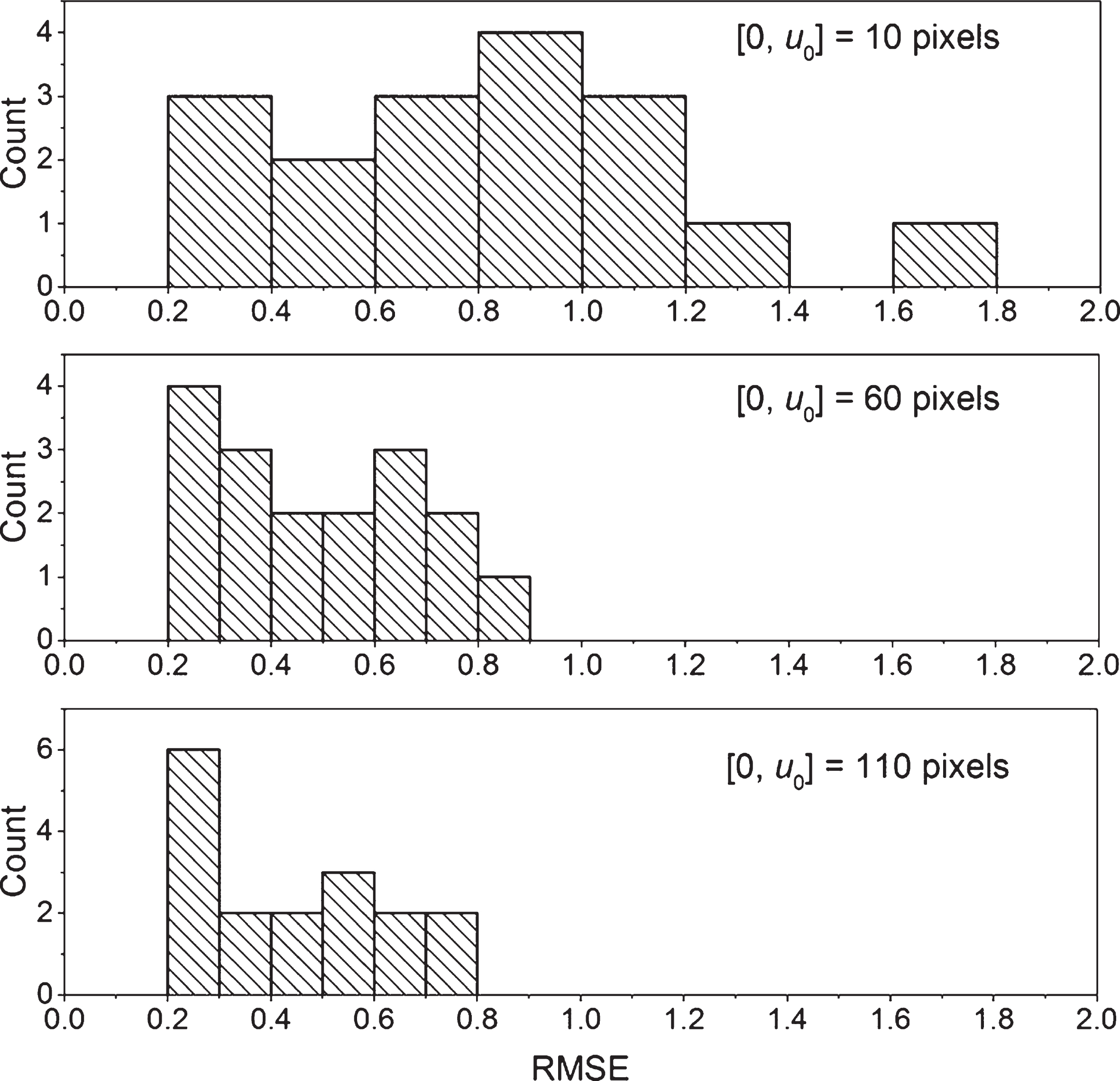
Histograms of RMSE for Δθ = 0 .25° (top panel, [0, u₀] = 10 pixels), Δθ = 1 .49° (middle panel, [0, u₀]= 60 pixels), and Δθ = 2 .72° (bottom panel, [0, u₀]= 110 pixels) are shown. There is progressive reduction in RMSE with increasing Δθ.

3.3 Effect of breast diameter on the RMSE

Figure 8 shows the scatter plot of the RMSE as a function of effective diameter of the breast at the chest-wall for (A) Δθ = 0 .25°, (B) Δθ = 1 .49°, and (C) Δθ = 2 .72°. The mean (±standard deviation) and median [range] of effective breast diameters were 17.96 (±1.97) cm and 17.33 [15.01 –22.1] cm, respectively. This indicates the range of breast diameters investigated in this study correspond to breasts larger than the average [45] or the median [29] reported in prior studies. As indicated earlier, relatively large breasts were included in this study so as to accommodate (128 voxels)³ VOI for power spectral analysis. The distribution of breast diameters satisfied the normality assumption (p = 0.344, Shapiro-Wilk’s test). Breast diameter was not correlated (Pearson correlation coefficient, r) with the RMSE for Δθ = 0 .25° (r = 0.173, p = 0.508) and for Δθ = 1 .49° (r = 0.46,p = 0.063), but was correlated for Δθ = 2 .72° (r = 0.494, p = 0.044).

Fig. 8

Scatter plots of the RMSE as a function of the effective diameter of the breast at the chest-wall are shown for (A) Δθ = 0 .25°, (B) Δθ = 1 .49°, and (C) Δθ = 2 .72°. The effective diameters of the breasts included in this study ranged from 15 to 22 cm and correspond to relatively large breasts.

3.4 Effect of breast off-center position on the RMSE

Figure 9 shows the scatter plot of the RMSE as a function of off-center position determined as the Euclidean distance between the AOR and the centroid of the chest-wall slice for (A) Δθ = 0 .25°, (B) Δθ = 1 .49°, and (C) Δθ = 2 .72°. The mean (±standard deviation) and median [range] of off-center breast position were 2.91 (±1.33) cm and 2.67 [1 – 5.1] cm, respectively. The distribution of off-center breast position satisfied the normality assumption (p = 0.277, Shapiro-Wilk’s test). Off-center breast position was statistically correlated with the RMSE for Δθ = 0 .25° (r = 0.507,p = 0.038), but was not correlated with the RMSE for Δθ = 1 .49° (r = 0.276,p = 0.284) and for Δθ = 2 .72° (r = 0.208,p = 0.424).

Fig. 9

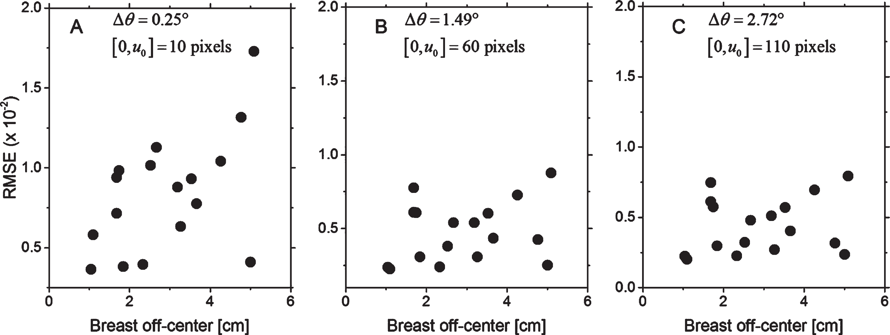
Scatter plots of the RMSE as a function of off-center position determined as the Euclidean distance between the AOR and the centroid of the chest-wall slice are shown for (A) Δθ = 0 .25°, (B) Δθ = 1 .49°, and (C) Δθ = 2 .72°.

3.5 Effect of fibroglandular volume fraction on the RMSE

The fibroglandular volume fraction denoted as VGF was obtained from a prior work [29] for the cases included in this study. The mean (±standard deviation) and median [range] of VGF for the cases included in this study were 0.15 (±0.15) cm and 0.07 [0.02 – 0.54], respectively. The VGF was log-transformed to satisfy the normality assumption (p = 0.373, Shapiro-Wilk’s test). Figure 10 shows the scatter plot of the RMSE as a function of log-transformed VGF for (A) Δθ = 0 .25°, (B) Δθ = 1 .49°, and (C) Δθ = 2 .72°. For each Δθ, the VGF did not exhibit statistical correlation with the RMSE (p > 0.481).

Fig. 10

Scatter plots of the RMSE as a function of log-transformed volumetric fibroglandular fraction (VGF) are shown for (A) Δθ = 0 .25°, (B) Δθ = 1 .49°, and (C) Δθ = 2 .72°.

3.6 Quantitative evaluation using absolute difference

At each Δθ, the summary metrics for the absolute difference (Diff) between full-projection CBBCT and truncated-projection CBBCT computed over the entire breast volume were identical across the three weighting schemes. Hence, only the Diff from truncated-projection CBBCT using Cho’s weighting scheme is reported (Table 2). For increasing Δθ, there is a decrease in the Diff (p = 1.37 × 10^-9, Wilks Lambda, repeated measures ANOVA). However, the differences are in the order of 10^-4 that is 2-3 orders of magnitude lower than the range of linear attenuation coefficients relevant to breast imaging and translates to less than±2 HU, for the specified spectrum. For Δθ = 2 .72°, Diff was not correlated with the effective diameter of the breast at chest-wall, off-center positioning of the breast and the volumetric fibroglandular fraction (p > 0.078). The above analysis indicates that the absolute difference (Diff) between full-projection CBBCT and truncated-projection CBBCT computed over the entire breast volume are nearly identical.

Table 2
Summary metrics of Diff (×10^-4; units of μ, cm^-1) computed over the entire breast volume with the full-fan reconstruction as the reference (SD – standard deviation; Min – Minimum; Q1 – 1st quartile; Q3 – 3rd Quartile; Max – Maximum). Δθ of 0 . 25°, 1 . 49° and 2 . 72° correspond to half-overlap regions [0, u₀] of 10, 60 and 110 pixels of 0.388 mm, respectively. Diff reduces with increasing Δθ and are similar for the three weighting schemes at each Δθ

Δθ Mean SD Min Q1 Median Q3 Max

0.25° 5.53 1.32 3.65 4.39 5.34 6.65 8.47

1.49° 5.14 1.31 3.36 3.99 4.90 6.17 8.14

2.72° 4.95 1.34 3.16 3.83 4.64 5.82 8.14

Δθ	Mean	SD	Min	Q1	Median	Q3	Max
0.25°	5.53	1.32	3.65	4.39	5.34	6.65	8.47
1.49°	5.14	1.31	3.36	3.99	4.90	6.17	8.14
2.72°	4.95	1.34	3.16	3.83	4.64	5.82	8.14

3.7 Quantitative power spectral analysis

The RMSE metric used in the aforementioned quantitative analyses provides an understanding of the deviation between the full-projection CBBCT and the truncated-projection CBBCT emulating the laterally-shifted detector geometry. However, it does not provide for spatial and consequently spatial-frequency dependent variations between the reconstructions. PS_Diff analysis of the difference between the CBBCT reconstructions of the full-projection and the truncated-projection datasets addresses this need. Also the PS_Diff corresponding to the chest-wall to nipple direction allows determination of whether there are cone-angle dependent effects for the truncated CBBCT relative to full-fan CBBCT. As noted earlier, the PS_Diff was computed from 3-D matched VOIs extracted from each case and from each reconstruction, followed by computing the difference between the full-projection CBBCT and the truncated-projection CBBCT prior to Fourier transformation. Figure 11 shows the 2-D PS_Diff extracted along the 3 orthogonal planes (columns in figure) from the 3-D PS_Diff for Δθ = 0 .25°, and each row corresponds to the 3 weighting schemes investigated. The planes (f_x, f_y), (f_x, f_z) and (f_y, f_z) correspond to the coronal, axial and sagittal planes, respectively. For the coronal plane (f_x, f_y), periodic artifacts are observed along the radial frequencies. For the axial and sagittal planes, they appear along the f_x and f_y axes; however, off-axis artifacts were not observed. Similar to the observation for the RMSE, the PS_Diff did not differ between the 3 weighting schemes. Hence, subsequent analyses are restricted to reconstructions using Cho’s weights and the observations are equally applicable to reconstructions using Schafer’s and Wang’s weights.

Fig. 11

For Δθ = 0 .25°, the 2-D PS_Diff extracted along the 3 orthogonal planes (columns) from the 3-D PS_Diff computed from the difference between the full cone-beam and the truncated cone-beam reconstructions are shown. Each row corresponds to the 3 weighting schemes investigated and the PS_Diff for each plane were identical.

Figure 12 shows the 2-D PS_Diff extracted along the 3 orthogonal planes (columns in figure) for Δθ = 0 .25° (top row), Δθ = 1 .49° (middle row), and Δθ = 2 .72° (bottom row). For Δθ = 1 .49° and Δθ = 2 .72°, the 2-D PS_Diff do not show any off-axis noise source along the 3 orthogonal planes. This implies that there is no structural noise component due to truncated-projection CBBCT when Δθ and consequently the half-overlap region [0, u₀] are appropriately chosen. The amplitude at the origin in the 2-D PS_Diff indicates spatially-invariant differences between the full-projection CBBCT and the truncated-projection CBBCT reconstructions that is consistent with the observations for Diff in Table 2.

Fig. 12

The 2-D PS_Diff extracted along the 3 orthogonal planes (columns in figure) for Δθ = 0 .25° (top row), Δθ = 1 .49° (middle row), and Δθ = 2 .72° (bottom row). For Δθ = 1 .49° and Δθ = 2 .72°, the 2-D PS_Diff do not show any off-axis noise source along the 3 orthogonal planes.

Figure 13 shows the 1-D PS_Diff along the 3 orthogonal axes extracted from the 3-D PS_Diff. Panels A through C provide the 1-D PS_Diff along each of the 3 axes and within each panel the plots correspond to the 3 Δθ values. Panel D provides the comparison of the 1-D PS_Diff along the 3 orthogonal spatial frequency axes for Δθ = 2 .72° that corresponds to half-overlap region of [0, u₀] = 110 pixels. For panels A and B, and to a lesser extent in panel C, there is progressive reduction in PS_Diff with increasing Δθ. In panel A and B that correspond to f_x and f_y axes respectively, periodic patterns are observed for Δθ = 0 .25°. In panel C that corresponds to f_z axis (cone-angle direction), such a pattern is not observed for Δθ = 0 .25°, as the cone-beam truncation is along the fan-angle and the weights are applied along the detector u-coordinate. In panel D corresponding to Δθ = 2 .72°, the 1-D PS_Diff is similar along the 3 spatial frequency axes. With the exception at near zero-spatial frequency, no peaks were observed along the 3 axes, indicating that the truncated-projection CBBCT does not distort or cause artifacts compared to the full-projection CBBCT. At spatial frequencies >0.3 cycles/mm, the PS_Diff amplitude is of the order of 10^-14 μ² mm³, where μ is the linear attenuation coefficient in units of cm^-1. At near-zero spatial frequency, the PS_Diff amplitude is of the order of 10^-8 μ² mm³, which is consistent with the estimate of Diff after accounting for voxel dimension (0.273 mm). The above analyses demonstrate that with appropriate selection of Δθ, artifact-free reconstruction is possible with the laterally-shifted detector approach. Additionally, the 1-D PS_Diff along the f_z axis show that cone-angle dependent effects are not substantially different between the full-projection and the truncated-projection CBBCT.

Fig. 13

The 1-D PS_Diff along the 3 orthogonal spatial frequency axes extracted from the 3-D PS_Diff are shown. A through C provide the 1-D PS_Diff along f_x, f_y and f_z, respectively and within each panel the plots correspond to the 3 Δθ values investigated. Panel D compares the 1-D PS_Diff along the 3 orthogonal spatial frequency axes for Δθ = 2 .72° that corresponds to half-overlap region of [0, u₀] = 110 pixels.

4 Discussion

Qualitative visual analysis showed that with appropriate selection of Δθ, CBBCT reconstructions of truncated projections emulating laterally-shifted detector geometry can provide similar images as full-projection CBBCT. Lesions of interest such as soft tissue abnormality and microcalcification cluster could be easily discerned. The study observed that for CBBCT using laterally-shifted detector geometry, the choice of weighting scheme used with pre-weighting FDK reconstruction algorithm did not impact either the RMSE or the PS_Diff. However, this observation may not be generalizable for imaging of other organs or anatomical locations. Quantitative evaluation showed progressive reduction in the RMSE and the PS_Diff with increasing Δθ. It is important to recognize that if the distances R and D in Fig. 2 are maintained, the 29 cm dimension of a 29 cm×23 cm detector can cover a fan angle of θ_max + Δθ, where θ_max = 12 . 47° and Δθ = 5 .81°, to provide a reconstructed FOV in the coronal plane matched to the 40 cm dimension of a 40 cm×30 cm detector. The maximum Δθ = 2 .72° considered in this study is substantially lower than 5 . 81°, indicating further reduction in the RMSE and the PS_Diff is possible.

For Δθ = 2 .72° that corresponds to half-overlap region [0, u₀] = 110 pixels of 0.388 mm pixel pitch in the detector plane, the mean RMSE (unit of μ, cm^-1) was 4.39 × 10^-3 indicating that quantitatively similar images as full-projection CBBCT is achievable with the laterally-shifted detector approach. For Δθ = 2 .72°, the maximum RMSE of 7.94 × 10^-3 corresponds to a large breast with effective diameter of 18.2 cm. Since the study observed a statistically significant and positive correlation between the breast diameter and the RMSE for Δθ = 2 .72°, and considering that the study included above average breast diameters, the mean RMSE for a typical breast diameter distribution encountered during clinical use is likely to be even smaller than the 4.39 × 10^-3 observed in this study. The study included a relatively wide range of off-center breast positions and did not observe a statistical correlation between the RMSE and the off-center breast position for Δθ = 2 .72°. Hence, it is unlikely that the off-center breast position could contribute to an increase in the RMSE. Also the volumetric glandular fraction VGF, often referred to as volumetric breast density, was not correlated with the RMSE and hence it is unlikely to impact the RMSE.

The analyses using PS_Diff showed that for Δθ = 2 .72°, the amplitude was in the order of 10^-14 μ² mm³, except near the origin, and did not contain any noticeable peaks indicating the lack of artifacts. However, for Δθ = 0 .25° artifacts in image domain (Fig. 3) as well as periodic patterns in the PS_Diff along the f_x and f_y axes (Fig. 13) were observed. The relatively small number of pixels in the overlap region for Δθ = 0 .25° is likely to be a contributing factor. Assuming the distances R and D in Fig. 2 are maintained, the proposed CMOS detector with a native pixel pitch of 0.075 mm and operated in 2×2 binned mode with pixel pitch of 0.15 mm, would provide half-overlap regions [0, u₀] ={ 25, 185, 255 } pixels for Δθ ={ 0 . 25°, 1 . 49°, 2 . 72° }. In comparison, the clinical dataset using in this study with Δθ ={ 0 . 25°, 1 . 49°, 2 . 72° } correspond to half-overlap regions [0, u₀] ={ 10, 60, 120 } pixels. The increased number of pixels for the same Δθ with the CMOS detector provides more number of data points (samples) for weighting and could further improve image quality.

While the study emulated laterally-shifted detector geometry by truncating the full cone-beam projection datasets along the fan-angle direction, it is important to recognize that the benefits of truncated cone-beam geometry in terms of reduced x-ray scatter [13] and reduction in radiation dose [40] cannot be realized in this study. In spite of these factors favoring full-projection CBBCT, the observation that CBBCT using laterally-shifted detector geometry can provide for similar image quality is highly promising. Additionally, the benefits of the proposed detector in terms of higher resolution and lower electronic or system noise could only be realized by developing such a CBBCT system.

It should also be clarified that we purposely targeted a smaller lateral dimension for the detector in this study (20 to 24 cm) than that currently available (29 to 30 cm), so that the air-gap between the breast and the detector can be increased for x-ray scatter rejection to improve quantitative accuracy, while maintaining the same reconstructed FOV. Based on the results from this study, the system magnification can be increased to 1.66 from 1.38. Monte Carlo simulations of radiation dose and x-ray scatter are subject of ongoing investigations which are necessary precursors for task-specific optimization of system geometry and will be reported in the future.

5 Conclusions

In this study, the feasibility of CBBCT with truncated cone-beam projections arising from smaller field-of-view detectors used in laterally-shifted detector geometry was investigated in terms of artifacts, visualization of lesions and quantitative evaluation using clinical data from patients that provide for real anatomical backgrounds and lesions. To our knowledge there have been no prior studies investigating laterally-shifted detector geometry for CBBCT using clinical datasets. Results from this study show that CBBCT with laterally-shifted detector geometry is feasible and that it can provide for artifact-free reconstruction with qualitatively and quantitatively similar images as full cone-beam breast CT. Additionally, the study showed that cone-angle dependent effects are not substantially different between full-fan CBBCT and truncated-fan CBBCT using laterally-shifted detector geometry. Considering that smaller FOV (30 cm×30 cm), high-resolution detectors with reduced dead-space at chest wall and lower noise characteristics are available, this study provides scientific evidence for pursuing research using the laterally-shifted detector approach to overcome the limited field of view and to address the major concerns with current CBBCT systems in terms of chest-wall coverage and visibility of microcalcifications. Additionally, this approach can improve quantitative accuracy by reducing the x-ray scatter contribution and has the potential to reduce the radiation dose.

Disclosures/Conflicts

All other authors have no conflicts related to this study.

Footnotes

Acknowledgments

This work was supported in part by National Institutes of Health (NIH) grants R21 CA134128 and R01 CA199044. The contents are solely the responsibility of the authors and do not represent the official views of the NIH or the National Cancer Institute. Preliminary and partial contents of this work were presented at the 55th Annual Meeting of the American Association of Physicists in Medicine (AAPM), Indianapolis, August 2013 and at the 4th International Conference on Image Formation in Computed Tomography (CT Meeting), Bamberg, Germany.

References

Niklason

L.T.

, Christian

B.T.

, Niklason

L.E.

, et al., Digital tomosynthesis in breast imaging, Radiology 205(2) (1997), 399–406.

Suryanarayanan

, Karellas

, Vedantham

, et al., Comparison of tomosynthesis methods used with digital mammography, Acad Radiol 7(12) (2000), 1085–1097.

Suryanarayanan

, Karellas

, Vedantham

, et al., Evaluation of linear and nonlinear tomosynthetic reconstruction methods in digital mammography, Acad Radiol 8(3) (2001), 219–224.

Sechopoulos

, Suryanarayanan

, Vedantham

, et al., Computation of the glandular radiation dose in digital tomosynthesis of the breast, Med Phys 34(1) (2007), 221–232.

Sechopoulos

, Suryanarayanan

, Vedantham

, et al., Scatter radiation in digital tomosynthesis of the breast, Med Phys 34(2) (2007), 564–576.

Vedantham

, Karellas

, Vijayaraghavan

G.R.

and Kopans

D.B.

, Digital Breast Tomosynthesis: State of the Art, Radiology 277(3) (2015), 663–684.

Sujlana

P.S.

, Mahesh

, Vedantham

, et al., Digital breast tomosynthesis: Image acquisition principles and artifacts, Clin Imaging 55 (2019), 188–195.

Lindfors

K.K.

, Boone

J.M.

, Nelson

T.R.

, et al., Dedicated breast CT: initial clinical experience, Radiology 246(3) (2008), 725–733.

Sechopoulos

, Vedantham

, Suryanarayanan

, et al., Monte Carlo and phantom study of the radiation dose to the body from dedicated CT of the breast, Radiology 247(1) (2008), 98–105.

10.

Crotty

D.J.

, McKinley

R.L.

and Tornai

M.P.

, Experimental spectral measurements of heavy K-edge filtered beams for x-ray computed mammotomography, Phys Med Biol 52(3) (2007), 603–616.

11.

Kalender

W.A.

, Beister

, Boone

J.M.

, et al., High-resolution spiral CT of the breast at very low dose: concept and feasibility considerations, Eur Radiol 22(1) (2012), 1–8.

12.

Vedantham

, Shi

, Karellas

and Noo

, Dedicated breast CT: radiation dose for circle-plus-line trajectory, Med Phys 39(3) (2012), 1530–1541.

13.

Mettivier

, Russo

, Lanconelli

and Meo

S.L.

, Cone-beam breast computed tomography with a displaced flat panel detector array, Med Phys 39(5) (2012), 2805–2819.

14.

Shen

, Zhong

, Lai

C.J.

, et al., Cone beam breast CT with a high pitch (75 mum), thick (500 mum) scintillator CMOS flat panel detector: visibility of simulated microcalcifications, Med Phys 40(10) (2013), 101915.

15.

O’Connell

, Conover

D.L.

, Zhang

, et al., Cone-beam CT for breast imaging: Radiation dose, breast coverage, and image quality, AJR Am J Roentgenol 195(2) (2010), 496–509.

16.

Prionas

N.D.

, Lindfors

K.K.

, Ray

, et al., Contrast-enhanced dedicated breast CT: initial clinical experience, Radiology 256(3) (2010), 714–723.

17.

O’Connell

A.M.

, Karellas

and Vedantham

, The potential role of dedicated 3D breast CT as a diagnostic tool: review and early clinical examples, Breast J 20(6) (2014), 592–605.

18.

Vedantham

, O’Connell

A.M.

, Shi

, et al., Dedicated Breast CT: Feasibility for Monitoring Neoadjuvant Chemotherapy Treatment, J Clin Imaging Sci 4 (2014), 64.

19.

Seifert

, Conover

, Zhang

, et al., Evaluation of malignant breast lesions in the diagnostic setting with cone beam breast computed tomography (Breast CT): feasibility study, Breast J 20(4) (2014), 364–374.

20.

O’Connell

A.M.

, Karellas

, Vedantham

, et al., Newer technologies in breast cancer imaging: Dedicated cone-beam breast computed tomography, Seminars in ultrasound, CT, and MR 39(1) (2018), 106–113.

21.

Cole

E.B.

, Campbell

A.S.

, Vedantham

, et al., Clinical performance of dedicated breast computed tomography in comparison to diagnostic digital mammography [abstract # SSA01-09]. 101st Scientific Assembly and Annual Meeting of the Radiological Society of North America November 29 - December 4; Chicago, IL, 2015.

22.

Vedantham

, Shi

, Karellas

, et al., Personalized estimates of radiation dose from dedicated breast CT in a diagnostic population and comparison with diagnostic mammography, Phys Med Biol 58(22) (2013), 7921–7936.

23.

Bian

, Yang

, Boone

J.M.

, et al., Investigation of iterative image reconstruction in low-dose breast CT, Phys Med Biol 59(11) (2014), 2659–2685.

24.

O’Connor

J.M.

, Glick

S.J.

, Gong

, et al., Characterization of a prototype table-top x-ray CT breast imaging system, Proc SPIE (2007), 65102T.

25.

Gazi

P.M.

, Yang

, Burkett

G.W.

Jr, , et al., Evolution of spatial resolution in breast CT at UC Davis, Med Phys 42(4) (2015), 1973–1981.

26.

Yang

, Huang

S.Y.

, Packard

N.J.

and Boone

J.M.

, Noise variance analysis using a flat panel x-ray detector: a method for additive noise assessment with application to breast CT applications, Med Phys 37(7) (2010), 3527–3537.

27.

Konstantinidis

A.C.

, Szafraniec

M.B.

, Rigon

, et al., X-ray Performance Evaluation of the Dexela CMOS APS X-ray Detector Using Monochromatic Synchrotron Radiation in the Mammographic Energy Range, IEEE Trans Nucl Sci 60(5) (2013), 3969–3980.

28.

Vedantham

, Karellas

, Emmons

M.M.

, et al., Dedicated breast CT: geometric design considerations to maximize posterior breast coverage, Phys Med Biol 58(12) (2013), 4099–4118.

29.

Vedantham

, Shi

, Karellas

, O’Connell

A.M.

, Dedicated breast CT: fibroglandular volume measurements in a diagnostic population, Med Phys 39(12) (2012), 7317–7328.

30.

Feldkamp

L.A.

, Davis

L.C.

and Kress

J.W.

, Practical Cone-Beam Algorithm, Journal of the Optical Society of America a-Optics Image Science and Vision 1(6) (1984), 612–619.

31.

Cho

P.S.

, Johnson

R.H.

and Griffin

T.W.

, Cone-beam CT for radiotherapy applications, Phys Med Biol 40(11) (1995), 1863–1883.

32.

Cho

P.S.

, Rudd

A.D.

and Johnson

R.H.

, Cone-beam CT from width-truncated projections, Comput Med Imaging Graph 20(1) (1996), 49–57.

33.

Wang

, X-ray micro-CT with a displaced detector array, Med Phys 29(7) (2002), 1634–1636.

34.

Schafer

, Grass

and van de Haar

, FBP and BPF reconstruction methods for circular X-ray tomography with off-center detector, Med Phys 38(Suppl 1) (2011), S85.

35.

Clackdoyle

, Noo

, Guo

J.Y.

and Roberts

J.A.

, Quantitative reconstruction from truncated projections in classical tomography, IEEE Trans Nucl Sci 51(5) (2004), 2570–2578.

36.

Bian

, Wang

, Han

, et al., Optimization-based image reconstruction from sparse-view data in offset-detector CBCT, Phys Med Biol 58(2) (2013), 205–230.

37.

Jaffray

D.A.

, Siewerdsen

J.H.

, Wong

J.W.

and Martinez

A.A.

, Flat-panel cone-beam computed tomography for image-guided radiation therapy, Int J Radiat Oncol Biol Phys 53(5) (2002), 1337–1349.

38.

Sowards-Emmerd

, Balakrishnan

, Wiener

, Lingxiong

and Jinghan

, editors. CBCT-subsystem performance of the multi-modality Brightview XCT system (M09-26). Nuclear Science Symposium Conference Record (NSS/MIC), IEEE; Oct. 24 - Nov. 1 2009.

39.

Vedantham

, Konate

, Shi

, et al., Dedicated cone-beam breast CT with laterally shifted CMOS detector. The 4th International Conference on Image Formation in X-ray Computed Tomography; July 18-22, 2016; Bamberg, Germany. pp. 291-4.

40.

Konate

, Vedantham

, Shi

and Karellas

, Radiation dose reduction and image quality evaluation of coronal truncated projections in cone-beam dedicated breast CT [abstract]. 2013 AAPM Annual Meeting Program, Indianapolis, IN Med Phys 40(6) (2013), 124.

41.

Shi

, Vedantham

, Karellas

and O’Connell

A.M.

, Skin thickness measurements using high-resolution flat-panel cone-beam dedicated breast CT, Med Phys 40(3) (2013), 031913.

42.

Shi

, Vedantham

, Karellas

and Zhu

, The role of off-focus radiation in scatter correction for dedicated cone beam breast CT, Med Phys 45(1) (2018), 191–201.

43.

Shi

, Vedantham

, Karellas

and Zhu

, Library based x-ray scatter correction for dedicated cone beam breast CT, Med Phys 43(8) (2016), 4529.

44.

Shi

, Vedantham

, Karellas

and Zhu

, X-ray scatter correction for dedicated cone beam breast CT using a forward-projection model, Med Phys 44(6) (2017), 2312–2320.

45.

Huang

S.Y.

, Boone

J.M.

, Yang

, et al., The characterization of breast anatomical metrics using dedicated breast CT, Med Phys 38(4) (2011), 2180–2191.