A new weighting scheme for arc based circle cone-beam CT reconstruction

Abstract

In this paper, we present an arc based fan-beam computed tomography (CT) reconstruction algorithm by applying Katsevich’s helical CT image reconstruction formula to 2D fan-beam CT scanning data. Specifically, we propose a new weighting function to deal with the redundant data. Our weighting function $ϖ (\underline{x}, λ)$ is an average of two characteristic functions, where each characteristic function indicates whether the projection data of the scanning angle contributes to the intensity of the pixel $\underline{x}$ . In fact, for every pixel $\underline{x}$ , our method uses the projection data of two scanning angle intervals to reconstruct its intensity, where one interval contains the starting angle and another contains the end angle. Each interval corresponds to a characteristic function. By extending the fan-beam algorithm to the circle cone-beam geometry, we also obtain a new circle cone-beam CT reconstruction algorithm. To verify the effectiveness of our method, the simulated experiments are performed for 2D fan-beam geometry with straight line detectors and 3D circle cone-beam geometry with flat-plan detectors, where the simulated sinograms are generated by the open-source software “ASTRA toolbox.” We compare our method with the other existing algorithms. Our experimental results show that our new method yields the lowest root-mean-square-error (RMSE) and the highest structural-similarity (SSIM) for both reconstructed 2D and 3D fan-beam CT images.

1 Introduction

Computed tomography (CT) has been widely used in clinical diagnosis and industrial applications because of its ability of providing inner vision of an object without destructing it. In classical tomography, the fan-beam CT reconstruction algorithm is fundamental since it can be heuristically extended to 3D helical cone-beam [1 –6] and circle cone-beam [7 –12] CT reconstructions. The standard fan-beam reconstruction method is the ramp filtered back-projection (FBP) algorithm [13, 14], which can be derived from the Radon inversion formula. For 2D CT image reconstruction, to reconstruct the whole image exactly and stably, it requires to measure all the line integrals of the X-rays that diverge from all directions and pass through the object. To make a fan-beam CT that samples data on a circular trajectory meet this condition, the detector must be large enough to cover the fan-angle of ±γ_m = arcsin(R _m/R _o) to avoid truncated projections and the X-ray source must travel on a continuous arc of π + 2γ_m on the circle to ensure that the line integrals of the X-rays diverging from all directions in the 2D plane and passing through the object are measured, where R _o is the radius of the scanning trajectory and R _m < R _o is the radius of the object. In the literature, the range of π + 2γ_m is called as short-scan.

To avoid completing the projection data of the remain angles ([π + 2γ_m : 2π]) and implement the reconstruction algorithm efficiently, Parker [15] proposed a weighting function to weight the short-scan fan-beam projection data before convoluting it. When the range of scanning angles is larger than the short-scan, redundant projection data is measured. Silver [16] extended Parker’s weighting function by utilizing the virtual detectors to tackle these redundant projection data.

In 2002, Noo et al. [17] proposed another type of FBP algorithm for fan-beam CT reconstruction by decomposing the convolution of the ramp filter into a successive convolution of a Hilbert filter and a derivative filter. After that, many other algorithms [9 , 19] based on the Hilbert transform were proposed. One advantage of these new algorithms is that they can exactly reconstruct a part of the image even though the range of the scanning angles is less than the short scan. These new algorithms can be seen as special cases that applying the 3D exact helical cone-beam inversion formula [20 –22] to the 2D CT reconstructions. To deal with the redundant data, a continuous weight function [9, 17] was also proposed to weight the filtered sinograms. In [23], Nett et al. derived a new algorithm for circle cone-beam CT reconstruction by applying Katsevich’s helical cone-beam algorithm [22] to circle con-beam geometry. They also proposed a structure factor weighting function to process the redundant data.

In summary, there exist mainly about three types of weighting functions in the literature. One is Parker’s [15] weighting function used in the conventional FBP [13, 14] algorithm and Feldkamp-Davis-Kress (FDK) [7] algorithm. Parker’s weighting function is assumed to be continuous and satisfy the normalization condition: $w_{1} (λ, γ) + w_{1} (λ + π - 2 γ, - γ) = 1$ (1) and Parker gave an explicit expression satisfying this condition: $w_{1} (λ, γ) = {\begin{matrix} {sin}^{2} (\frac{π}{4} \frac{λ}{γ_{m} + γ}) & if 0 ⩽ λ < 2 (γ_{m} + γ) \\ 1 & if 2 (γ_{m} + γ) ⩽ λ < π + 2 γ, \\ {sin}^{2} (\frac{π}{4} \frac{π + 2 γ_{m} - λ}{γ_{m} - γ}) & if π + 2 γ ⩽ λ < π + 2 γ_{m} \\ 0 & if π + 2 γ_{m} ⩽ λ < 2 π \end{matrix}$ (2) where λ is the rotation scanning angle of the X-ray source, γ is the diverging angle of the X-ray beam, ±γ_m = arcsin(R _m/R _o) is the fan-angle, R _o is the radius of the source trajectory and R _m < R _o is the radius of the object to be imaged.

Another is Noo’s weighting function used in their reconstruction algorithms [9, 17] and has the following expression: $w_{2} (λ, γ) = \frac{c (λ)}{c (λ) + c (λ + π - 2 γ)}$ (3) where $c (λ) = {\begin{matrix} {cos}^{2} \frac{π (λ - λ_{s} - d)}{2 d} & if λ_{s} < λ < λ_{s} + d, \\ 1 & if λ_{s} + d < λ < λ_{e} - d, \\ {cos}^{2} \frac{π (λ - λ_{e} + d)}{2 d} & if λ_{e} - d < λ < λ_{e} \end{matrix}$ (4) and λ_s and λ_e are the starting and ending angles of the scan and d is a super-parameter such that c (λ) smoothly drops from 1 to 0.

The third type weighting function is Nett’s function [23] used for circle cone-beam CT. The weighting function for image points ${\underline{x}}_{off}$ outside the scanning plane formed by the source trajectory can be expressed as

$c_{h} ({\underline{x}}_{off}, λ) = 1 c_{i} ({\underline{x}}_{off}, λ) = {\begin{matrix} - \frac{1}{2}, & if λ \in T_{3} ({\underline{x}}_{off}), \\ \frac{1}{2}, & if λ \in T_{1} ({\underline{x}}_{off}) \cup T_{2} ({\vec{x}}_{off}), \end{matrix} c_{f} ({\underline{x}}_{off}, λ) = {\begin{matrix} - \frac{1}{2}, & if λ \in T_{1} ({\underline{x}}_{off}), \\ \frac{1}{2}, & if λ \in T_{2} ({\underline{x}}_{off}) \cup T_{3} ({\underline{x}}_{off}), \end{matrix}$ (5)

and for the image points ${\underline{x}}_{in}$ in the scanning plane is $c_{i} ({\underline{x}}_{in}, λ) = {\begin{matrix} 2, & if λ \in T_{2} ({\underline{x}}_{in}), \\ 1, & if λ \in T_{1} ({\underline{x}}_{in}) \cup T_{3} ({\vec{x}}_{in}), \end{matrix}$ (6)

where the subscript “h” indicates that the filtering direction is horizontal, the subscript “i” or “f” indicates that the filtering line is determined by the critical plane that is perpendicular to the scanning plane and passes through the initial or final source point, respectively and T ₁, T ₂ and T ₃ are three regions of the source trajectory, where there are one intersection point between the critical plane and T ₂, and two intersection points between the critical plane and T ₁ or T ₃.

In this paper, we first present an arc based algorithm for fan-beam CT reconstruction by applying Katsevich’s helical CT [21] formula to 2D fan-beam CT. Then, we propose a new weighting function to tackle the redundant projection data. Our weighting function $ϖ (\underline{x}, λ)$ is the average of two characteristic functions with respective to the scanning angle λ, where each characteristic function indicates that whether the projection data of the scanning angle contributes to the intensity of the pixel $\underline{x}$ in the CT images. In fact, for every pixel $\underline{x}$ , our method uses the projection data of two scanning angle intervals to reconstruct its intensity, where one interval contains the starting angle and the other contains the end angle, and each interval corresponds to a characteristic function. By extending the weighted arc based fan-beam algorithm to the circle cone-beam geometry, we also obtain a new circle cone-beam CT reconstruction algorithm.

Parker’s [15] weighting function w ₁ (λ, γ) and Noo’s [17] weighting function w ₂ (λ, γ) depend on the scanning angle λ and the diverging angle γ, and are required to be continuous with respective to them. When discretizing the reconstruction formulas, the continuity condition may result in more discretization errors. Moreover, a super-parameter d exists in Noo’s [23] weighting function, which greatly influences the qualities of reconstructed CT images. For circle cone-beam CT, the optimal value of d for each slice of the CT image may be different and so is somewhat hard to tune.

For our method, the weighting function $w (\underline{x}, λ)$ depends on λ and the pixel position $\underline{x}$ , which has no continuity constraint on γ. Besides, compared to Noo’s weighting function, ours has no super-parameter. Nett’s weighting function has the same variables of ours, but for circle cone-beam CT, the definitions are different and the derived reconstructing formula (defined in (14)) with our weighting function (26) is more simper than that defined in (19) of Nett’s [23].

2 Methods

2.1 Katsevich’s helical cone-beam formula

Katsevich [21] proposed an exact reconstruction formula for helical cone-beam CT and Noo et al. [24] researched how to implement it efficiently and accurately. The reconstruction formula can be written as $f (\underline{x}) = - \frac{1}{2 π} \int_{λ_{0} (\underline{x})}^{λ_{p} (\underline{x})} d λ \frac{1}{∥ \underline{x} - \underline{a} (λ) ∥} g^{F} (λ, \frac{\underline{x} - \underline{a} (λ)}{∥ \underline{x} - \underline{a} (λ) ∥})$ (7)

where $λ_{0} (\underline{x})$ and $λ_{p} (\underline{x})$ are the extremities of the π-line passing through $\underline{x}$ with $λ_{0} (\underline{x}) < λ_{p} (\underline{x})$ , $\underline{a} (λ)$ is the helical trajectory formed by the X-ray source position, $g^{F} (λ, \underline{θ}) = \int_{0}^{2 π} d γ h_{H} (sin γ) g^{'} (λ, cos γ \underline{θ} + sin γ (\underline{θ} \times \underline{m} (λ, \underline{θ}))),$ (8) $g^{'} (λ, \underline{θ}) = lim_{ɛ \to 0} \frac{g (λ + ɛ, \underline{θ}) - g (λ, \underline{θ})}{ɛ},$ (9) $h_{H} (s) = - \int_{- \infty}^{+ \infty} d σ i sign (σ) e^{i 2 π σ s} = \frac{1}{π s}$ (10)

is the Hilbert filter, $g (λ, \underline{θ})$ is the measured projection data, vector $\underline{m} (λ, \underline{θ})$ is normal to the κ-plane K (λ, ψ) of the smallest |ψ| value that contains the line of direction $\underline{θ}$ through $\underline{a} (λ)$ and the κ-plane K (λ, ψ) is any 2D plane that has three intersections $\underline{a} (λ)$ , $\underline{a} (λ + ψ)$ and $\underline{a} (λ + 2 ψ)$ with the helix, where ψ ∈ (- π, π).

2.2 ARC based fan-beam algorithm

Applying (7) to the 2D fan-beam reconstruction, the π-line becomes a chord of the circle of the scanning trajectory, the κ-plane K (λ, ψ) coincides with the image plane to reconstruct and so $\underline{θ} \times \underline{m} (λ, \underline{θ}) = {\underline{θ}}^{⊥}$ .

Let $\underline{a} (λ) = (R_{o} cos λ, R_{o} sin λ)$ be the position of the X-ray source on the trajectory circle of radius R _o and $g (λ, \underline{θ}) = \int_{0}^{+ \infty} d tf (\underline{a} (λ) + t \underline{θ})$ (11) be the measured projection data, where $\underline{θ} \in S^{1}$ is a diverging direction of the X-ray and S ¹ is the unit circle on the 2D plane. Then, according to (7), the reconstruction formula for fan-beam CT can be written as $f (\underline{x}) = - \frac{1}{2 π} \int_{λ_{1} (\underline{x})}^{λ_{2} (\underline{x})} d λ \frac{1}{∥ \underline{x} - \underline{a} (λ) ∥} g^{F} (λ, \frac{\underline{x} - \underline{a} (λ)}{∥ \underline{x} - \underline{a} (λ) ∥})$ (12)

where $[λ_{1} (\underline{x}), λ_{2} (\underline{x})]$ is an interval in R such that the three points $\underline{a} (λ_{1} (\underline{x}))$ , $\underline{a} (λ_{2} (\underline{x}))$ and $\underline{x}$ are in a straight line (i.e. $\underline{x}$ is on the chord formed by $\underline{a} (λ_{1} (\underline{x}))$ and $\underline{a} (λ_{2} (\underline{x}))$ ), $| \underline{x} | < R_{m} < R_{o}$ , R _m is the radius of the test object, $g^{F} (λ, \underline{θ}) = \int_{0}^{2 π} d \bar{γ} h_{H} (sin \bar{γ}) g^{'} (λ, cos \bar{γ} \underline{θ} + sin \bar{γ} {\underline{θ}}^{⊥})$ (13) h _H (s) and $g^{'} (λ, \underline{θ})$ are defined by (10) and (9), respectively.

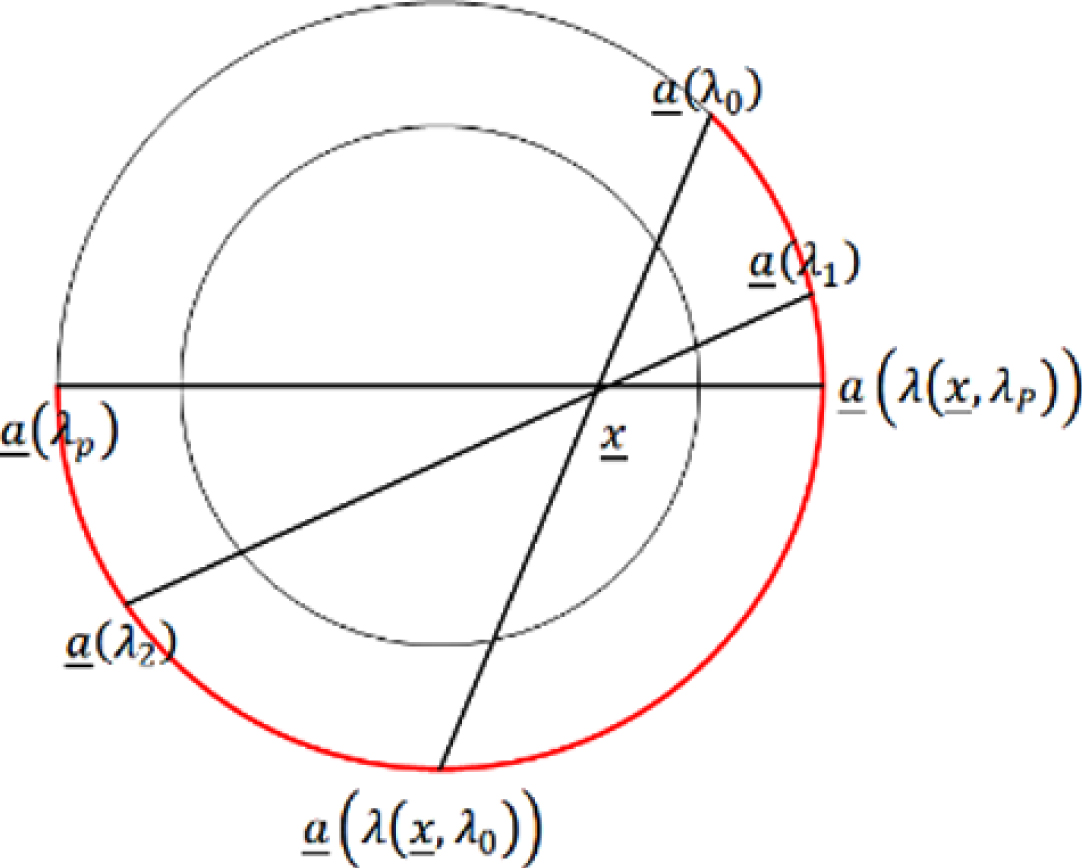
For any fixed $\underline{x}$ in the trajectory circle, there may exist many available chords passing through $\underline{x}$ and so the integral lower and upper limits can be different (see Fig. 1). Moreover, when the range of the scanning arc is equal or larger than the short scan, redundant projection data needs to be processed. A simple method to tackle these redundant projection data is to calculate (12) for all available intervals and average them, which may smooth some details of the reconstructed image. In this paper we only consider two types of angle intervals corresponding to the chords that respectively pass through the two endpoints of the scanning arcs.

Fig. 1

Demonstration that to reconstruct the density of pixel $\underline{x}$ , the integral can be done on any of the arcs $\overset{︷}{\underline{a} (λ_{0}), \underline{a} (λ (\underline{x}, λ_{0}))}$ , $\overset{︷}{\underline{a} (λ (\underline{x}, λ_{P})), \underline{a} (λ_{P})}$ or $\overset{︷}{\underline{a} (λ_{1}), \underline{a} (λ_{2})}$ , respectively.

Therefore, we propose the following formula for fan-beam reconstruction: $f (\underline{x}) = - \frac{1}{2 π} \int_{λ_{0}}^{λ_{P}} d λ \frac{ϖ (\underline{x}, λ)}{∥ \underline{x} - \underline{a} (λ) ∥} g^{F} (λ, \frac{\underline{x} - \underline{a} (λ)}{∥ \underline{x} - \underline{a} (λ) ∥}),$ (14)

where λ₀ < λ_P correspond to the two endpoints of the scanning arcs, $ϖ (\underline{x}, λ) = \frac{1}{2} (ϖ_{1} (\underline{x}, λ) + ϖ_{2} (\underline{x}, λ))$ (15)

is a weighting function, and $ϖ_{1} (\underline{x}, λ)$ and $ϖ_{2} (\underline{x}, λ)$ are defined by

$ϖ_{1} (\underline{x}, λ) = {\begin{matrix} 1, if \underline{a} (λ) \in \overset{︷}{\underline{a} (λ_{0}), \underline{a} (λ (\underline{x}, λ_{0}))}, \\ 0 else, \end{matrix} ϖ_{1} (\underline{x}, λ) = {\begin{matrix} 1, if \underline{a} (λ) \in \overset{︷}{\underline{a} (λ (\underline{x}, λ_{p})), \underline{a} (λ_{p})}, \\ 0 else, \end{matrix}$ (16)

where $\underline{a} (λ (\underline{x}, λ_{0}))$ is another endpoint of the chord passing through $\underline{a} (λ_{0})$ and $\underline{x}$ , $\underline{a} (λ (\underline{x}, λ_{P}))$ is another endpoint of the chord passing through $\underline{a} (λ_{P})$ and $\underline{x}$ , and $\overset{︷}{\underline{a} (λ_{0}), \underline{a} (λ (\underline{x}, λ_{0}))}$ denotes the arc starting from $\underline{a} (λ_{0})$ and ending at $\underline{a} (λ (\underline{x}, λ_{0}))$ . Note that (14) is very similar to (4) in [25], but the weighting functions are different.

2.2.1 Implementation for curved-line detectors

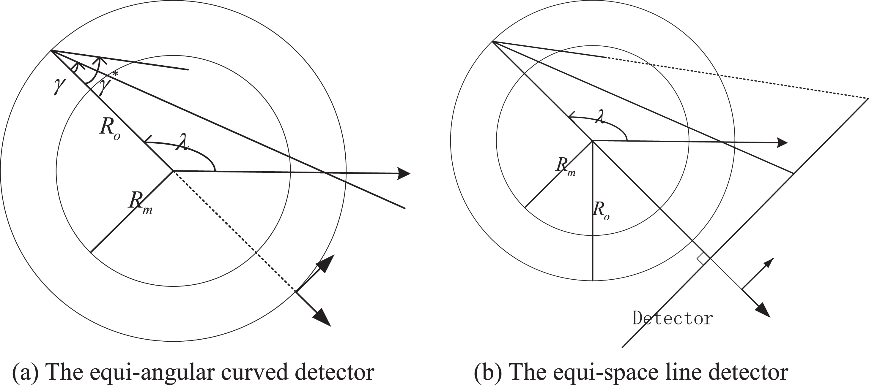
In this subsection, we describe how to implement (14) when the fan-beam projections are measured by using an equi-angular curved-line detector. Let $\underline{a} (λ) = (R_{o} cos λ, R_{o} sin λ)$ be the position of the X-ray source, $\underline{θ} (λ, γ) = cos γ {\underline{e}}_{0} (λ) + sin γ {\underline{e}}_{1} (λ)$ be the diverging direction, $g_{c} (λ, γ) = g (λ, \underline{θ} (λ, γ))$ be the measured projection data using the curved-line detector, where γ is the sampling coordinate of the fan-angle, ${\underline{e}}_{0} (λ) = (- sin (λ), cos (λ))$ , ${\underline{e}}_{1} (λ) = (- cos (λ), - sin (λ))$ (See Fig. 2a). By the chain rule [17], (9) can be implemented as $g_{1} (λ, γ) : = g^{'} (λ, \underline{θ} (λ, γ)) = \frac{\partial g_{c} (λ, γ)}{\partial λ} + \frac{\partial g_{c} (λ, γ)}{\partial γ} .$ (17)

Fig. 2

Geometries of data acquisition for 2D fan-beam CT.

Applying the changes of variable $\bar{γ} = γ^{'} - γ$ , (13) can be rewritten as $g_{2} (λ, γ) : = g^{F} (λ, \underline{θ} (λ, γ)) = - \int_{0}^{2 π} d γ^{'} h_{H} (sin (γ - γ^{'})) g_{1} (λ, γ^{'}) .$ (18)

Let $γ^{*} (\underline{x}, λ) = arctan (\frac{\underline{x} \cdot {\underline{e}}_{0} (λ)}{R_{o} + \underline{x} \cdot {\underline{e}}_{1} (λ)})$ be the fan angle of the measured X-ray that diverges from $\underline{a} (λ)$ and passes through $\underline{x}$ . Then, (14) can be rewritten as $f (\underline{x}) = - \frac{1}{2 π} \int_{λ_{0}}^{λ_{P}} d λ \frac{ϖ (\underline{x}, λ)}{∥ \underline{x} - \underline{a} (λ) ∥} g_{2} (λ, γ^{*}) .$ (19)

Compared to the classical FBP algorithm, (19) needs to calculate the extra weighting function $ϖ (\underline{x}, λ)$ and multiply the filtered sinogram g ₂ (λ, γ) by $ϖ (\underline{x}, λ)$ . The weighting function $ϖ (\underline{x}, λ)$ can be pre-calculated only once and stored in the memory. The computational cost of multiplying g ₂ (λ, γ) by $ϖ (\underline{x}, λ)$ is equal to that of multiplying g ₂ (λ, γ) by $\frac{1}{∥ \underline{x} - \underline{a} (λ) ∥}$ in the FBP algorithm. Therefore, (19) doesn’t significantly increase the computational cost.

2.2.2 Implementation for straight-line detectors

In this subsection, we show how to implement the algorithm for the fan-beam projections measured by using an equi-space straight-line detector. Let $\underline{a} (λ) = (R_{o} cos λ, R_{o} sin λ)$ be the position of the X-ray source, $\underline{θ} (λ, u) = \frac{u {\underline{e}}_{0} (λ) + D {\underline{e}}_{1} (λ)}{\sqrt{u^{2} + D^{2}}}$ be the diverging direction, $g_{l} (λ, u) = g (λ, \underline{θ} (λ, u))$ be the measured projection data using the straight-line detector, where u is the sampling coordinate parallel to the detector, D is the distance between the X-ray source and the detector, ${\underline{e}}_{0} (λ) = (- sin (λ), cos (λ))$ , ${\underline{e}}_{1} (λ) = (- cos (λ), - sin (λ))$ (See Fig. 2b). By the chain rule, (9) can be implemented as $g_{1} (λ, u) : = g^{'} (λ, \underline{θ} (λ, u)) = \frac{\partial g_{l} (λ, u)}{\partial λ} + \frac{u^{2} + D^{2}}{D} \frac{\partial g_{l} (λ, u)}{\partial u} .$ (20)

Applying the changes of variables u = D tan(γ) and $\bar{u} = D tan (γ^{'})$ , (18) and (19) can be respectively rewritten as $g_{2} (λ, u) : = g^{F} (λ, \underline{θ} (λ, u)) = - \int_{- u_{m}}^{u_{m}} d \bar{u} \frac{D}{\sqrt{{\bar{u}}^{2} + D^{2}}} h_{H} (u - \bar{u}) g_{1} (λ, \bar{u})$ (21) and $f (\underline{x}) = - \frac{1}{2 π} \int_{λ_{0}}^{λ_{P}} d λ \frac{ϖ (\underline{x}, λ)}{R_{o} + \underline{x} \cdot {\underline{e}}_{1} (λ)} g_{2} (λ, u^{*}),$ (22)

where u _m = D tan γ_m, γ_m = arcsin(R _m/R _o) and $u^{*} (\underline{x}, λ) = D \frac{\underline{x} \cdot {\underline{e}}_{0} (λ)}{R_{o} + \underline{x} \cdot {\underline{e}}_{1} (λ)}$ is the detector location of the measured X-ray that diverges from $\underline{a} (λ)$ and passes through $\underline{x}$ .

2.3 Circle cone-beam algorithm

Equation (14) can be extended for circle cone-beam CT reconstructions heuristically. In the following, we give the detailed circle cone-beam reconstruction algorithms for flat-plane and curve-plane detectors, respectively.

2.3.1 Implementation for flat-plane detectors

Let $\underline{a} (λ) = (R_{0} cos (λ), R_{0} cos (λ), 0)$ be the position of the X-ray source, (u, v, w) be the local detector coordinates with unit vectors

${\underline{e}}_{u} (λ) = (- sin (λ), cos (λ), 0), {\underline{e}}_{v} (λ) = (- cos (λ), - sin (λ), 0), {\underline{e}}_{w} (λ) = (0, 0, 1),$ (23)

and $g_{f} (λ, u, w) = g (λ, \underline{θ} (λ, u, w))$ be the measured projection data by using a flat-plane detector with diverging direction $\underline{θ} (λ, u, w) = \frac{u {\underline{e}}_{u} (λ) + D {\underline{e}}_{v} (λ) + w {\underline{e}}_{w} (λ)}{\sqrt{u^{2} + D^{2} + w^{2}}},$ (24)

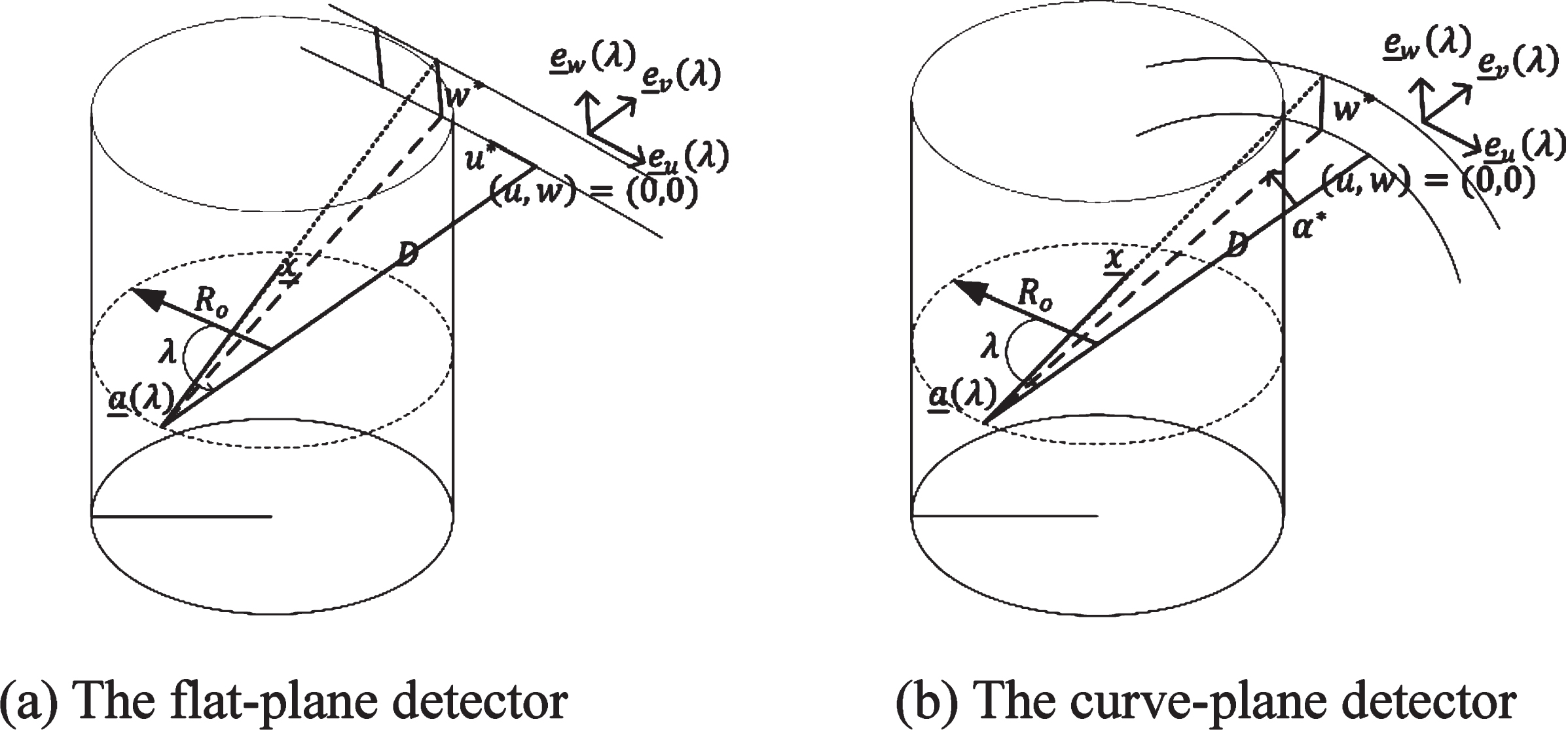
where D is the distance between the detector plane and the X-ray source (See Fig. 3a). To make (14) effective for the circle cone-beam CT reconstruction, we need to modify ${\underline{θ}}^{⊥}$ in (13) and the weighting function $ϖ (\underline{x}, λ)$ in (15).

Fig. 3

Geometries of data acquisition for 3D circle cone-beam CT.

In this paper, we heuristically set ${\underline{θ}}^{⊥} (λ, u, w) = \underline{θ} (λ, u, w) \times (\frac{D {\underline{e}}_{v} (λ) + w {\underline{e}}_{w} (λ)}{\sqrt{D^{2} + w^{2}}} \times {\underline{e}}_{u} (λ))$ (25) and $ϖ_{3 d} (\underline{x}, λ) = ϖ (Proj (\underline{x}), λ)$ (26)

where $Proj (\underline{x})$ represents projecting $\underline{x}$ on the circle plane formed by the trajectory of the X-ray source. Then, as derived in Appendix A, the circle cone-beam reconstruction algorithm for the flat-plane detector can be implemented as follows.

step1: derivative at constant direction

$g_{1} (λ, u, w) : = g^{'} (λ, \underline{θ} (λ, u, w)) = \frac{g_{f} (λ, u, w)}{\partial λ} + \frac{u^{2} + D^{2}}{D} \frac{g_{f} (λ, u, w)}{\partial u} + \frac{uw}{D} \frac{g_{f} (λ, u, w)}{\partial w} .$ (27)

step2: convolution with Hilbert filter:

$g_{2} (λ, u, w) : = g^{F} (λ, \underline{θ} (λ, u, w)) = \int_{- u_{m}}^{u_{m}} d \bar{u} \frac{D}{\sqrt{{\bar{u}}^{2} + D^{2} + w^{2}}} h_{H} (u - \bar{u}) g_{1} (λ, \bar{u}, w),$ (28)

where u _m = D tan γ_m, γ_m = arcsin(R _m/R _o).

step3: backprojection $f (\underline{x}) = \frac{1}{2 π} \int_{λ_{0}}^{λ_{P}} d λ \frac{ϖ_{3 d} (\underline{x}, λ)}{v^{*} (\underline{x}, λ)} g_{2} (λ, u^{*}, w^{*})$ (29)

where $(u^{*} (\underline{x}, λ), w^{*} (\underline{x}, λ))$ is the position in the detector of the measured X-ray that diverges from $\underline{a} (λ)$ and passes through $\underline{x}$ , which can be calculated by

$\begin{matrix} v^{*} (\underline{x}, λ) = R_{o} + \underline{x} \cdot {\underline{e}}_{v} (λ), \\ u^{*} (\underline{x}, λ) = \frac{D}{v^{*} (\underline{x}, λ)} (\underline{x} \cdot {\underline{e}}_{u} (λ)), \\ w^{*} (\underline{x}, λ) = \frac{D}{v^{*} (\underline{x}, λ)} (\underline{x} \cdot {\underline{e}}_{w} (λ)) . \end{matrix}$ (30)

2.3.2 Implementation for curve-plane detectors

The curved-plane detector array consists of N _row × N _cols detectors. The detector columns are perpendicular to the trajectory circle of the X-ray source, while the detector rows form circle arcs parallel to each other and to the trajectory circle, where the center of the arc on the trajectory circle plane coincides with the X-ray source.

Let $\underline{a} (λ) = (R_{0} cos (λ), R_{0} cos (λ), 0)$ be the position of the X-ray source, (α, v, w) be the local detector coordinates with unit vectors defined in (23) and $g_{c} (λ, α, w) = g (λ, \underline{θ} (λ, α, w))$ be the measured projection data by using a curve-plane detector with diverging direction $\underline{θ} (λ, α, w) = \frac{D sin (α) {\underline{e}}_{u} (λ) + D cos (α) {\underline{e}}_{v} (λ) + w {\underline{e}}_{w} (λ)}{\sqrt{D^{2} + w^{2}}}$ (31)

where D is the distance between the detector plane and the X-ray source (See Fig. 3b). The curve-plane detector coordinates (α, v _c, w _c) can be converted to the flat detector coordinates (u, v _f, w _f) via $u = D tan (α), v_{f} = v_{c}, w_{f} = \frac{w_{c}}{cos (α)} .$ (32)

Applying the changes of variable in (32), we can obtain the circle cone-beam reconstruction algorithm for the curve-plane detector as follows.

step1: derivative at constant direction $g_{1} (λ, α, w) : = g^{'} (λ, \underline{θ} (λ, α, w)) = \frac{g_{c} (λ, α, w)}{\partial λ} + \frac{g_{c} (λ, α, w)}{\partial α} .$ (33)

step2: convolution with Hilbert filter:

$\begin{matrix} g_{2} (λ, α, w) : = g^{F} (λ, \underline{θ} (λ, α, w)) \\ = \int_{0}^{2 π} d \bar{α} \frac{D}{\sqrt{{\bar{D}}^{2} + w^{2}}} h_{H} (sin (α - \bar{α})) g_{1} (λ, \bar{α}, w) . \end{matrix}$ (34)

step3: back-projection $f (\underline{x}) = \frac{1}{2 π} \int_{λ_{0}}^{λ_{P}} d λ \frac{ϖ_{3 d} (\underline{x}, λ)}{v^{*} (\underline{x}, λ)} cos (α^{*}) g_{2} (λ, α^{*}, w^{*}),$ (35)

where $(α^{*} (\underline{x}, λ), w^{*} (\underline{x}, λ))$ is the position in the detector of the measured X-ray that diverges from $\underline{a} (λ)$ and passes through $\underline{x}$ , which can be calculated by

$\begin{matrix} v^{*} (\underline{x}, λ) = R_{o} + \underline{x} \cdot {\underline{e}}_{v} (λ), \\ α^{*} (\underline{x}, λ) = arctan (\frac{\underline{x} \cdot {\underline{e}}_{u} (λ)}{v^{*} (\underline{x}, λ)}), \\ w^{*} (\underline{x}, λ) = \frac{D cos (α^{*})}{v^{*} (\underline{x}, λ)} (\underline{x} \cdot {\underline{e}}_{w} (λ)) . \end{matrix}$ (36)

2.4 Additional discrete schemes

In order to implement our CT reconstruction algorithms, we need to give the discrete definitions of the derivatives $\frac{\partial g_{c} (λ, γ)}{\partial λ}$ and $\frac{\partial g_{c} (λ, γ)}{\partial γ}$ in (17), $\frac{\partial g_{l} (λ, u)}{\partial λ}$ and $\frac{\partial g_{l} (λ, u)}{\partial u}$ in (20), $\frac{g_{f} (λ, u, w)}{\partial λ}$ , $\frac{g_{f} (λ, u, w)}{\partial u}$ and $\frac{g_{f} (λ, u, w)}{\partial w}$ in (27), and $\frac{g_{c} (λ, α, w)}{\partial λ}$ and $\frac{g_{c} (λ, α, w)}{\partial α}$ in (33), the Hilbert filters h _H (u) in (21) and (28), h _H (sin(γ)) in (18) and h _H (sin(α)) in (34), and the weighting functions $ϖ_{1} (\underline{x}, λ)$ and $ϖ_{2} (\underline{x}, λ)$ in equation (16).

Let

$\begin{matrix} γ_{i} = i \nabla γ, i = - N, - N + 1, . . ., 0, . . ., N - 1, N, \\ α_{i} = i \nabla α, i = - N, - N + 1, . . ., 0, . . ., N - 1, N, \\ u_{j} = j \nabla u, j = - M, - M + 1, . . ., 0, . . ., M - 1, M, \\ w_{k} = k \nabla w, k = - L, - L + 1, . . ., 0, . . ., L - 1, L \end{matrix}$ (37) be the discrete coordinates of the detectors and $λ_{s} = s \nabla λ, s = 0, 1, . . ., P$ (38) be the discrete sampling angles. To avoid the space shift in the reconstructed images, we use the centered difference schemes to calculate the derivatives:

$\begin{matrix} \frac{\partial g_{c} (λ_{s}, γ)}{\partial λ} = \frac{g_{c} (λ_{s + 1}, γ) - g_{c} (λ_{s - 1}, γ)}{2 \nabla λ}, \\ \frac{\partial g_{c} (λ, γ_{i + 1 / 2})}{\partial γ} = \frac{g_{c} (λ, γ_{i + 1}) - g_{c} (λ, γ_{i})}{\nabla γ}, \\ \frac{\partial g_{l} (λ_{s}, u)}{\partial λ} = \frac{g_{l} (λ_{s + 1}, u) - g_{l} (λ_{s - 1}, u)}{2 \nabla λ}, \\ \frac{\partial g_{l} (λ, u_{j + 1 / 2})}{\partial λ} = \frac{g_{l} (λ, u_{j + 1}) - g_{l} (λ, u_{j})}{\nabla u}, \\ \frac{g_{f} (λ_{s}, u, w)}{\partial λ} = \frac{g_{f} (λ_{s + 1}, u, w) - g_{f} (λ_{s - 1}, u, w)}{2 \nabla λ}, \\ \frac{g_{f} (λ, u_{j + 1 / 2}, w)}{\partial u} = \frac{g_{f} (λ, u_{j + 1}, w) - g_{f} (λ, u_{j}, w)}{\nabla u}, \frac{g_{f} (λ, u, w_{k})}{\partial u} = \frac{g_{f} (λ, u, w_{k + 1}) - g_{f} (λ, u, w_{k - 1})}{2 \nabla w}, \\ \frac{g_{c} (λ_{s}, α, w)}{\partial λ} = \frac{g_{c} (λ_{s + 1}, α, w) - g_{c} (λ_{s - 1}, α, w)}{2 \nabla λ}, \\ \frac{g_{c} (λ, α_{i + 1 / 2}, w)}{\partial α} = \frac{g_{c} (λ, α_{i + 1}, w) - g_{c} (λ, α_{i}, w)}{\nabla α} . \end{matrix}$ (39)

The discrete definitions of the Hilbert filters are [26]:

$\begin{matrix} k_{H} (u_{j + 1 / 2}) = \frac{1 - cos (π u_{j + 1 / 2} / \nabla u)}{π u_{j + 1 / 2}}, \\ h_{H} (sin (γ_{i + 1 / 2})) = \frac{1 - cos (π γ_{i + 1 / 2} / \nabla γ)}{π sin (γ_{i + 1 / 2})}, \\ h_{H} (sin (α_{i + 1 / 2})) = \frac{1 - cos (π α_{i + 1 / 2} / \nabla α)}{π sin (α_{i + 1 / 2})} . \end{matrix}$ (40)

For the weighting functions $ϖ_{1} (\underline{x}, λ)$ and $ϖ_{2} (\underline{x}, λ)$ , since the endpoints $\underline{a} (λ (\underline{x}, λ_{0}))$ and $\underline{a} (λ (\underline{x}, λ_{P}))$ may not coincide with the sampling points a (λ_s), we need to interpolate them at the endpoints of the sampling angles $λ (\underline{x}, λ_{0})$ and $λ (\underline{x}, λ_{P})$ . Let

$\begin{matrix} s (\underline{x}, λ_{0}) = (λ (\underline{x}, λ_{0}) - λ_{0}) / \nabla λ, \\ ⌊ s (\underline{x}, λ_{0}) ⌋ = floor (s (\underline{x}, λ_{0})), \\ ⌈ s (\underline{x}, λ_{0}) ⌉ = floor (s (\underline{x}, λ_{0})) + 1, \\ s (\underline{x}, λ_{P}) = (λ (\underline{x}, λ_{P}) - λ_{0}) / \nabla λ, \\ ⌊ s (\underline{x}, λ_{P}) ⌋ = floor (s (\underline{x}, λ_{P})), \\ ⌈ s (\underline{x}, λ_{P}) ⌉ = floor (s (\underline{x}, λ_{P})) + 1 . \end{matrix}$ (41)

Then, we set

$ϖ_{1} (\underline{x}, λ_{s}) = {\begin{matrix} 1, if s \in [0, ⌊ s (\underline{x}, λ_{0}) ⌋], \\ s - ⌊ s (\underline{x}, λ_{0}) ⌋, if s \in (⌊ s (\underline{x}, λ_{0}) ⌋, ⌈ s (\underline{x}, λ_{0}) ⌉), \\ 0, else, \end{matrix} ϖ_{2} (\underline{x}, λ_{s}) = {\begin{matrix} 1, if s \in [⌊ s (\underline{x}, λ_{P}) ⌋, P], \\ s - ⌊ s (\underline{x}, λ_{P}) ⌋, if s \in (⌊ s (\underline{x}, λ_{P}) ⌋, ⌈ s (\underline{x}, λ_{P}) ⌉), \\ 0, else, \end{matrix}$ (42)

where $λ (\underline{x}, λ_{0})$ and $λ (\underline{x}, λ_{P})$ can be calculated via Appendix B.

3 Experimental results

In this section, we give some simulation results to verify the effectiveness of our algorithms. For 2D fan-beam CT reconstructions, we do the experiments on the simulated projection data measured by straight-line detectors while for 3D circle cone-beam, the simulated projection data measured by flat-plane detectors are used to reconstruct CT images. The codes for implementing our methods can be downloaded from https://github.com/wangwei-cmd/phantom.

3.1 Fan-beam with straight-line detectors

In this subsection, we present some CT images reconstructed from the fan-beam projection data measured by straight-line detectors and compare the results with those of the conventional fan-beam algorithm with Parker-extended weighting function (CFA) [16] and Noo’s algorithm (NOA) [17]. The CFA method is implemented by calling the “FBP-cuda” algorithm in the ASTRA Toolbox [27]. The codes for implementing the NOA and our method are almost the same except for the weighting functions. The hyper-parameter d in NOA [17] is set as d = 5π/180.

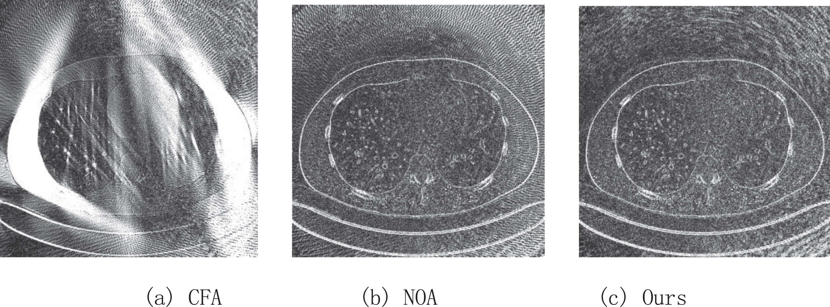
To estimate the performances of the three compared algorithms, the “astra_create_projector” function with parameter “line_fanflat” in the ASTRA Toolbox is used to generate the sinogram, where $λ = [0 : 1 : 220] \times \frac{π}{180}$ , D = 1363, R _o = 1000, the reconstructed volume is [-255.5 : 1 :255.5] × [-255.5 : 1 :255.5] and the position of the detector in the u coordinate is u = [-494 : 1 :494].

In Fig. 4, we show the CT images reconstructed by CFA, NOA and ours, respectively. We can observe that the left-top part of the CT image reconstructed by CFA is a little dark due to suffering the inhomogeneous intensity. To better observe the differences of the three reconstructed images, we present the absolute error images |f - g| in Fig. 5, where f is the reconstructed image and g is the ground truth. We can see that the intensity error of the image reconstructed by NOA is large and the image reconstructed by NOA has more stripe error at the four corners compared to that of our method.

Fig. 4

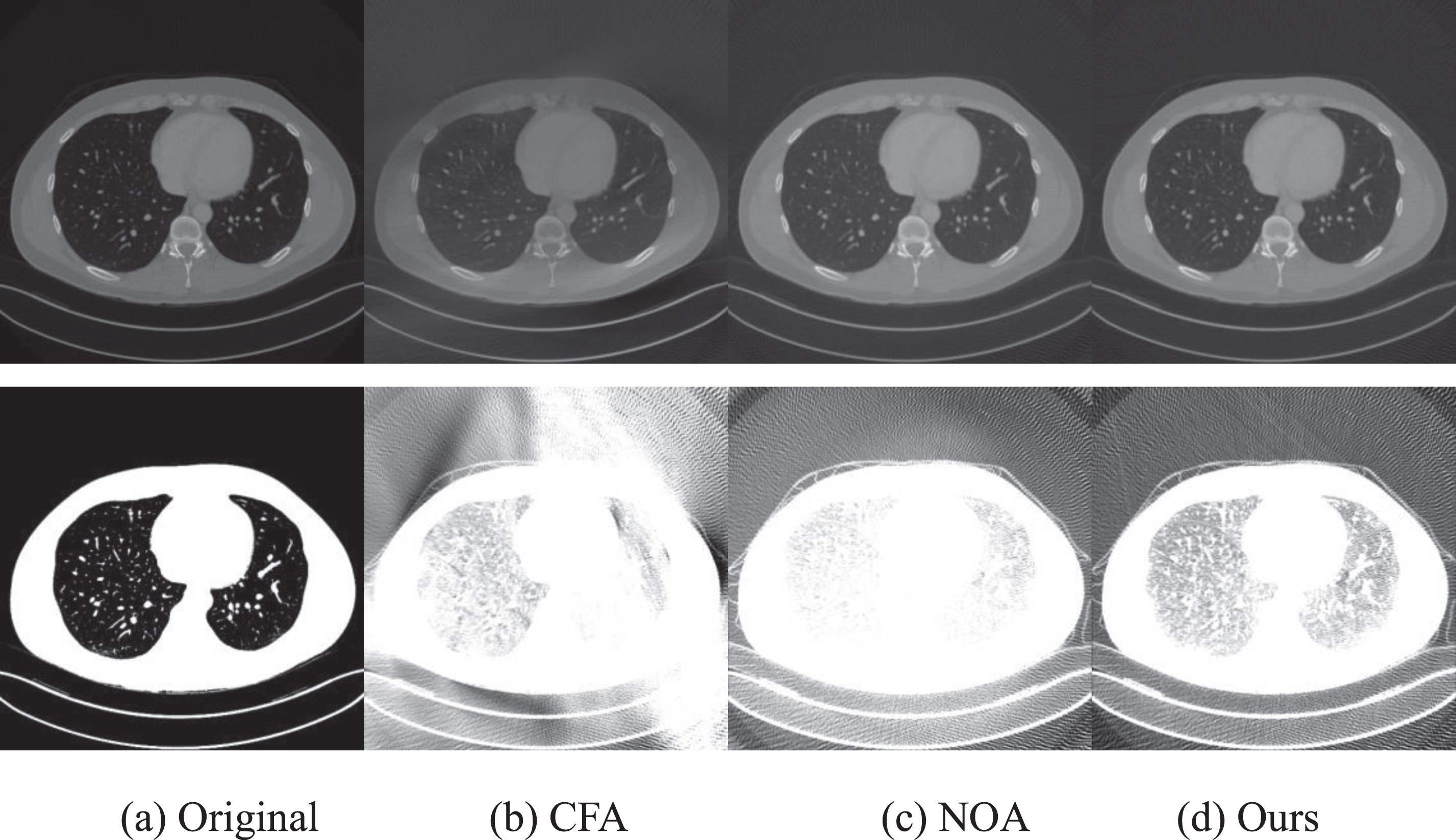
Reconstructed CT images from fan beam projections and their enhanced versions, where the intensities were linearly stretched in [0, 1] and the display widths of row 1 and row 2 are [0, 1] and [0.1, 0.2], respectively.

Fig. 5

Absolute error images of Fig. 4, where the intensities were linearly stretched in [0, 1] and the display width is [0.1, 0.15].

To estimate the results of the methods objectively, the root-mean-square-error (RMSE) and the structural-similarity (SSIM) of the three reconstructed CT images in Fig. 4 are list in Table 1, where the RMSE and SSIM between the reconstructed CT image f and the referenced image g are, respectively, defined as $RMSE = \sqrt{\frac{{∥ f - g ∥}_{2}^{2}}{n}}, SSIM = \frac{(2 μ_{1} μ_{2} + c_{1}) (2 σ_{1, 2} + c_{2})}{(μ_{1}^{2} + μ_{2}^{2} + c_{1}) (σ_{1}^{2} + σ_{2}^{2} + c_{2})},$ (43) μ₁ and μ₂ are the mean values of f and g, σ₁ and σ₂ are the variances of f and g, respectively, σ_1,2 is the covariance between f and g, C ₁ = (0.01 × (max(g) - min(g))) ² and C ₂ = (0.03 × (max(g) - min(g))) ², and n is the number of pixels. From Table 1, we can observe that our method has the least RMSE and largest SSIM.

Table 1

The RMSE and SSIM of CT Images in Fig. 4

RMSE	SSSIM
CFA	172.00	0.61
NOA	71.25	0.73
Ours	64.00	0.76

In investigating the robustness of our method to noise, we add different level “Gaussian+Poisson” noises to the sinogram via the following formulas [28]:

$g = exp (- g / M), g = g + I_{0} \times poission (g) + I_{0} \times Gaussin (m, var / I_{0}), g = log (I_{0} / g) \times M,$ (44)

where M is the maximal value of the projection data g, m = 0 and var are the mean and variance of the Gaussian noise, respectively, I ₀ = 10⁶ is the average photon count for the Poisson noise. Fig. 6 shows the reconstructed CT images from the noisy sinograms, where the corresponding variance parameters are var = 0.1, 1, 10, 100. From Fig. 6, we can observe that our method can reconstruct the CT images from the noisy sinograms.

Fig. 6

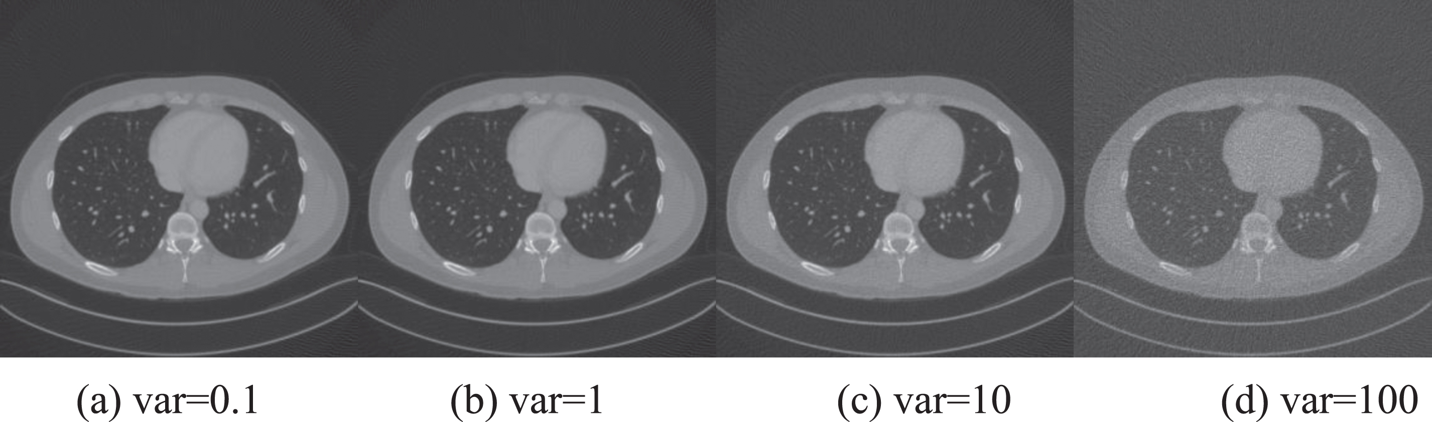
CT images reconstructed from noisy fan-beam projections with different variances.

To evaluate the spatial resolutions of the compared methods, a radial-stripe image is used as the test image and its corresponding sinogram is also generated by ASTRA Toolbox with the same parameters. In Fig. 7, the original radial-stripe image and the reconstructed images by the three methods are presented. We can see that the reconstructed images by NOA and ours have similar visual effects. Compared to NOA and ours, CFA have higher contrast, but it may over enhance the most center part of the test image. To better compare the three methods, two profile plots corresponding to the green circle and red circle in Fig. 7a are shown in Fig. 8. We can observe that the profile plots of Noo and ours almost coincide and the CFA tends to increase the intensity range of the reconstructed image. In Fig. 8a, the profile plot of CFA is more consistent with the original than those of Noo and ours but the opposite in Fig. 8b.

Fig. 7

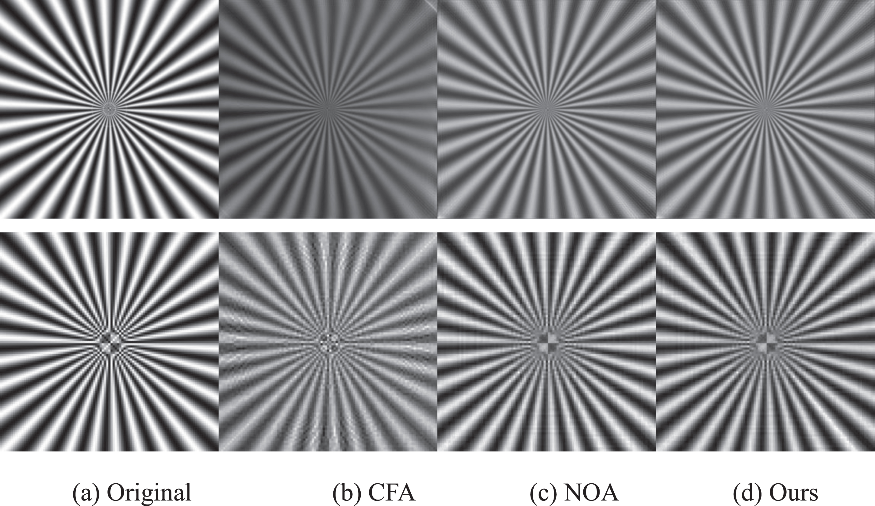
Radial-stripe images reconstructed by the three methods, where the images in second row are the enlargement of the center parts of images in the first row.

Fig. 8

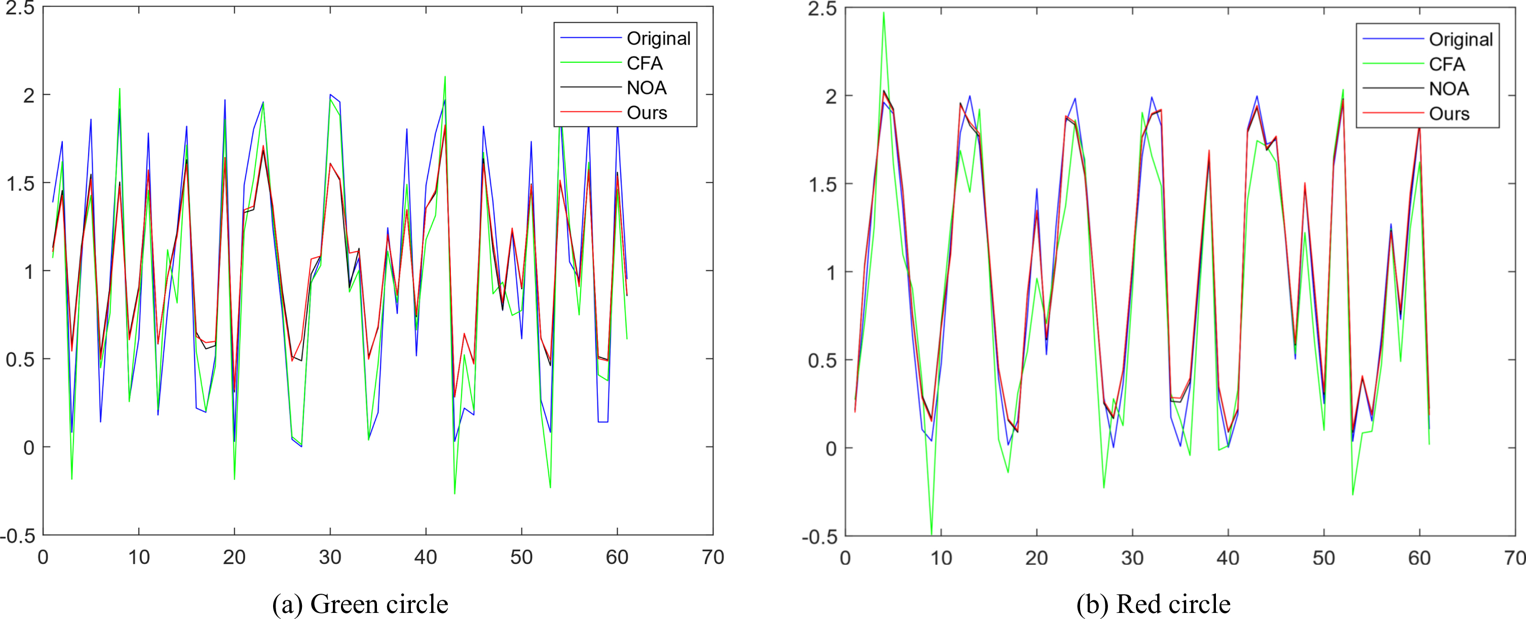
Profile plots corresponding to the green and red circles in Fig. 7a.

3.2 Circle cone-beam with flat-plane detectors

In this subsection, we give some CT images reconstructed from the circle cone-beam projection data measured by flat-plane detectors to verify the effectiveness of our method, and compare the results with those of the Feldkamp-Davis-Kress (FDK) algorithm [7] and Noo’s algorithm (NOA) [17], where we extend the weighting function of NOA such that it can be used to reconstruct circle cone-beam CT images.

The CFA method is implemented by calling the “FDK-CUDA” algorithm in the ASTRA Toolbox [27]. The codes for implementing the NOA and our method are also almost the same except for the weighting functions. The hyper-parameter d in NOA [17] is set as d = 8π/180.

We use 25 continuous CT images of size 512 × 512 from the “the 2016 NIH-AAPM-Mayo Clinic Low Dose CT Grand Challenge” [29] to resemble one test object. The parameters for the circle cone-beam CT with the flat-plane detector are set as follows: u = [-906 : 1 :906], v = [-76 : 1 :76], R _o = 500, D = 863 and λ = [0 : 1 :274] × π/180. The 13th slice of the object is assumed to lie in the plane z = 0 (i.e. the plane formed by the trajectory of the X-ray source). The “astra_create_proj_geom” function with parameter “cone” in the ASTRA Toolbox is used to generate the sinogram.

In Fig. 9, the 8th sliced images of the test object reconstructed by FDK, NOA and ours are presented. From Fig. 9b, we can observe that there exist some artifacts in the CT images reconstructed by FDK. Some discretization errors can be observed from Fig. 9c reconstructed by NOA. Compared to Fig. 9b and Fig. 9c, the CT image reconstructed by our method has less artifacts and discretization errors as can be observed in Fig. 9d. To better observe the differences of each CT images, the absolute error images of Fig. 9 are shown in Fig. 10, where we can observe that NOA has more stripe errors than ours.

Fig. 9

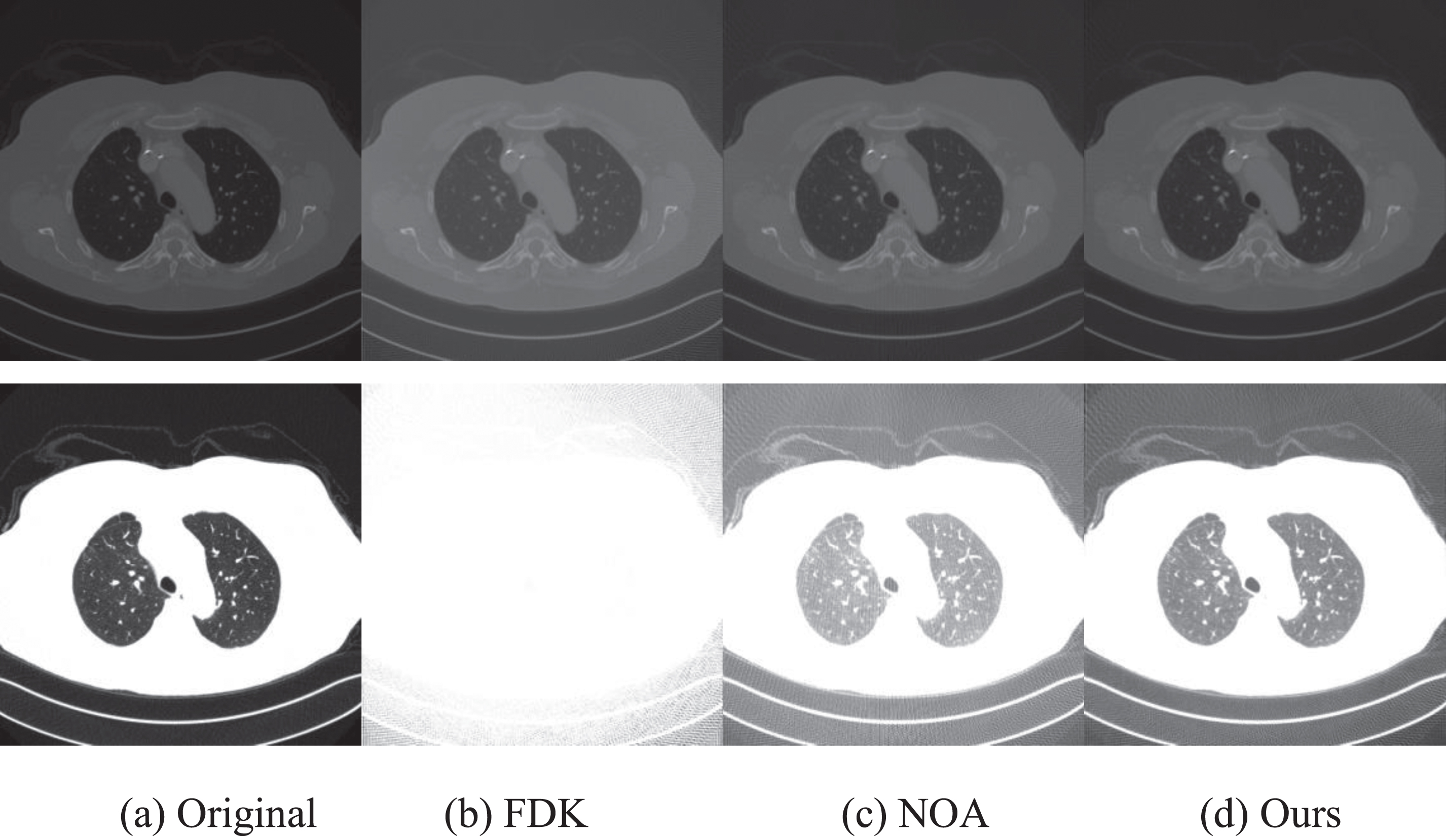
Sliced CT images reconstructed from circle cone-beam projection data and their enhanced versions, where the intensities were linearly stretched in [0, 1] and the display widths of row 1 and row 2 are [0, 1] and [0, 0.2], respectively.

Fig. 10

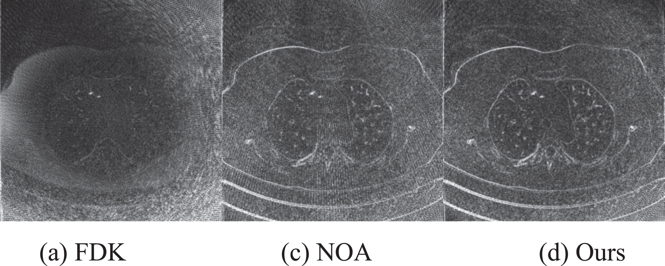
Absolute error images of Fig. 9, where the intensities were linearly stretched in [0, 1] and the display width is [0, 0.2].

In Table 2, we list the averaged RMSE and SSIM of the 25 reconstructed images by CFA, NOA and ours, respectively. We can observe that the CT images reconstructed by our method has the lowest RMSE and the largest SSIM in average.

Table 2

The averaged RMSE and SSIM of CT Images reconstructed by FDK, NOA and ours

	RMSE	SSSIM
FDK	158.19	0.57
NOA	131.43	0.63
Ours	121.15	0.70

4. Discussion and conclusion

In this paper, we proposed a new weighting function to deal with the redundant projection data for the arc based fan-beam CT algorithm, which was obtained by applying Katsevich’s helical CT formula [21] to 2D fan-beam CT reconstruction. By extending the arc based algorithm to circle cone-beam geometry with the proposed weighting function, we also obtained a new algorithm for circle cone-beam CT reconstruction. Experiments showed that our methods outperform the related algorithms for fan-beam and circle cone-beam CT reconstructions.

The main differences between Noo’s algorithm [17] and ours are the weighting functions. One advantage of our weighting function over Noo’s is that ours has no super parameter while Noo’s has a super-parameter d, which greatly influences its performance. Moreover, for circle cone-beam CT, the optimal value of d for each slice may be different and so is somewhat hard to tune.

Our study performs experiments only on the simulated data. The main differences of simulated CT and real CT are the ways to obtain the sinograms. For simulated CT, sinograms are generated by discretizing the line integral equation (11). For real CT, sinograms are obtained by measuring the intensities of the X-ray beam passing through the object, in which the measurements may be impacted by many factors and so the obtained sinograms are not strictly consistent with equation (11). For example in [30], the X-ray beam consisting of photons at different energies may result in estimating the photon numbers inaccurately; the detectors and the X-ray source are not real dots and thus the measured photons are from a bundle of lines rather than a single line; the photons from the source may be scattered and can’t reach the detectors. Besides, due to the properties of photons, noise is inevitable during the measuring process. Though there exist a lot of differences between the simulated data and real data, experiments on simulated data are still meaningful since it can not only verify the effectiveness of the proposed algorithm, but also enable us to investigate individually the impact of these factors that can’t be identified in real data.

Footnotes

Acknowledgments

This work was supported partly by National Natural Science Foundation of China (Nos.12001381, 61871274 and 61801305), Peacock Plan (No. KQTD2016053112051497), Shenzhen Key Basic Research Project (Nos. JCYJ20180507184647636, JCYJ20170412104656685, JCYJ2017081809410 9846, and JCYJ20190808155618806), Chongqing Natural Science Foundation of China (No. cstc2019jcyj-msxmX0060), key project of science and technology research program of Chongqing Education Commission of China (KJZD-K202001503).

Appendix A. Algorithm for circle cone-beam CT with flat-plane detectors

As can be observed from Fig. A-1, we obtain the following equations.

$\begin{matrix} {\underline{e}}_{u} (λ) = \frac{\vec{A_{4} A_{3}}}{| | \vec{A_{4} A_{3}} | |}, {\underline{e}}_{v} (λ) = \frac{\vec{A_{1} A_{2}}}{\vec{A_{1} A_{2}}}, {\underline{e}}_{w} (λ) = \frac{\vec{A_{2} A_{3}}}{\vec{A_{2} A_{3}}}, \\ | | \vec{A_{4} A_{3}} | | = u, | | \vec{A_{5} A_{3}} | | = \bar{u}, | | \vec{A_{2} A_{3}} | | = w, | | \vec{A_{2} A_{3}} | | = D, \\ ∠ A_{4} A_{1} A_{3} = α, ∠ A_{5} A_{1} A_{4} = \bar{γ} . A \end{matrix} . 1)$

We also have $tan (α + \bar{γ}) = \frac{| | \vec{A_{5} A_{3}} | |}{| | \vec{A_{1} A_{3}} | |} = \frac{\bar{u}}{\sqrt{D^{2} + w^{2}}}$ and so $d \bar{γ} = \frac{{cos}^{2} (α + \bar{γ})}{\sqrt{D^{2} + w^{2}}} d \bar{u} = \frac{\sqrt{D^{2} + w^{2}}}{D^{2} + w^{2} + {\bar{u}}^{2}} d \bar{u} . A . 2)$

By the Law of Sines, we have $sin \bar{γ} = | | \vec{A_{5} A_{4}} | | \frac{sin (∠ A_{1} A_{5} A_{3})}{| | \vec{A_{1} A_{4}} | |} = \frac{\sqrt{D^{2} + w^{2}} (\bar{u} - u)}{\sqrt{D^{2} + w^{2} + {\bar{u}}^{2}} \sqrt{D^{2} + w^{2} + u^{2}}} . A . 3)$

Therefore, $h_{H} (sin \bar{γ}) = \frac{\sqrt{D^{2} + w^{2} + {\bar{u}}^{2}} \sqrt{D^{2} + w^{2} + u^{2}}}{\sqrt{D^{2} + w^{2}}} h_{H} (\bar{u} - u) . A . 4)$

Note that $\underline{θ} (λ, u, w) = \frac{\vec{A_{1} A_{4}}}{| | \vec{A_{1} A_{4}} | |}$ and so $cos \bar{γ} \underline{θ} + sin \bar{γ} {\underline{θ}}^{⊥} = \frac{\vec{A_{1} A_{5}}}{| | \vec{A_{1} A_{5}} | |}$ . Substituting equations (A.2) and (A.4) into equation (13), we can obtain $\begin{matrix} g^{F} (λ, \underline{θ} (λ, u, w)) = \\ - \frac{\sqrt{u^{2} + D^{2} + w^{2}}}{D} \int_{- u_{m}}^{u_{m}} d \bar{u} \frac{D}{\sqrt{{\bar{u}}^{2} + D^{2} + w^{2}}} h_{H} (u - \bar{u}) g_{1} (λ, \bar{u}, w), A \end{matrix} . 5)$

From Fig. 3a, we can observe that $\begin{matrix} ∥ \underline{x} - \underline{a} (λ) ∥ = \sqrt{{(u^{*})}^{2} + {(w^{*})}^{2} + D^{2}} \frac{(\underline{x} - \underline{a} (λ)) \cdot {\underline{e}}_{v} (λ)}{D} \\ = \frac{\sqrt{{(u^{*})}^{2} + {(w^{*})}^{2} + D^{2}}}{D} (R_{o} + \underline{x} \cdot {\underline{e}}_{v} (λ)) . A \end{matrix} . 6)$

Substituting equation (A.6) into equation (12), we can get $f (\underline{x}) = - \frac{D}{\sqrt{D^{2} + {(w^{*})}^{2} + {(u^{*})}^{2}}} \frac{1}{2 π} \int_{λ_{0}}^{λ_{P}} d λ \frac{ϖ_{3 d} (\underline{x}, λ)}{v^{*} (\underline{x}, λ)} g_{2} (λ, u^{*}, w^{*}) . A . 7)$

Canceling the factors $- \frac{\sqrt{u^{2} + D^{2} + w^{2}}}{D}$ and $- \frac{D}{\sqrt{D^{2} + {(w^{*})}^{2} + {(u^{*})}^{2}}}$ in equations (A.5) and (A.7), we obtain the algorithm for circle cone-beam CT with the flat-plane detector.

Appendix B. Algorithm for calculating one endpoint of a chord

Let (R _o cos λ₀, R _o sin λ₀) and (R _o cos λ₁, R _o sin λ₁) be the two end-points of a chord on a circle with radius r = R _o and (x ₁, x ₂) be a point on the chord. Then, we have (B.1) $\begin{matrix} R_{o} (\cos λ_{1} - \cos λ_{0}) = t * (x_{1} - R_{o} \cos λ_{0}), \\ R_{o} (\sin λ_{1} - \sin λ_{0}) = t * (x_{2} - R_{o} \sin λ_{0}), \end{matrix}$

where t ∈ [0, 1]. Solving equation set (B.1), we have (B.2) $\begin{matrix} cos λ_{1} = \frac{(- R_{o}^{2} + x_{1}^{2} + x_{2}^{2}) cos λ_{0} - 2 x_{1} (- R_{o} + x_{1} cos λ_{0} + x_{2} sin λ_{0})}{R_{o}^{2} + x_{1}^{2} + x_{2}^{2} - 2 x_{1} R_{o} cos λ_{0} - 2 x_{2} R_{o} sin λ_{0}}, \\ sin λ_{1} = \frac{(- R_{o}^{2} + x_{1}^{2} + x_{2}^{2}) sin λ_{0} - 2 x_{2} (- R_{o} + x_{1} cos λ_{0} + x_{2} sin λ_{0})}{R_{o}^{2} + x_{1}^{2} + x_{2}^{2} - 2 x_{1} R_{o} cos λ_{0} - 2 x_{2} R_{o} sin λ_{0}} . B \end{matrix} . 1)$

Thus, we can get λ₁ by λ₁ = arccos(cos λ₁), where λ₁ needs to be changed by λ₁ = 2π - λ₁ when sin λ₁ < 0.

References

Wang

, Lin

T.H.P.C.

, et al., A general cone-beam reconstruction algorithm, IEEE Transactions on Medical Imaging 12(3) (1993), 486–496.

Stierstorfer

, Rauscher

, Boese

, et al., Weighted FBP –a simple approximate 3D FBP algorithm for multislice spiral CT with good dose usage for arbitrary pitch, Physics in Medicine and Biology 49(11) (2004), 2209–2218.

Noo

, Hoppe

, Dennerlein

, et al., A new scheme for view-dependent data differentiation in fan-beam and cone-beam computed tomography, Physics in Medicine and Biology 52(17) (2007), 5393–5414.

Zamyatin

A.A.

, Taguchi

and Silver

M.D.

, Practical hybrid convolution algorithm for helical CT reconstruction, IEEE Transactions on Nuclear Science 53(1) (2006), 167–174.

Tang

X.Y.

, Hsieh

, Nilsen

R.A.

, et al., A three-dimensional-weighted cone beam filtered backprojection (CB-FBP) algorithm for image reconstruction in volumetric CT –helical scanning, Physics in Medicine and Biology 51(4) (2006), 855–874.

Shi

, Liu

, Yu

, et al., Review of CT image reconstruction open source toolkits, Journal of X-ray Science and Technology 28(4) (2020), 619–639.

Feldkamp

, Davis

and Kress

, Practical cone-beam algorithm, Journal of the Optical Society of America a-Optics Image Science and Vision 1(6) (1984), 612–619.

L.F.

, Pan

X.C.

and Pelizzari

C.A.

, Image reconstruction with a shift-variant filtration in circular cone-beam CT, International Journal of Imaging Systems and Technology 14(5) (2004), 213–221.

Kudo

, Noo

, Defrise

and Clackdoyle

New super-short-scan algorithms for fan-beam and cone-beam reconstruction, in IEEE Nuclear Science Symposium and Medical Imaging Conference, (2003), 902–906.

10.

Tang

and Tang

, Axial cone-beam reconstruction by weighted BPF/DBPF and orthogonal buttery filtering, IEEE Transactions on Biomedical Engineering 63(9) (2016), 1895–1903.

11.

Tang

, Huang

, Cheng

, et al., Three-dimensional weighting in cone beam FBP reconstruction and its transformation over geometries, IEEE Transactions on Biomedical Engineering 65(6) (2018), 1235–1244.

12.

Matenine

, Schmittbuhl

, Bedwani

, et al., Iterative reconstruction for image enhancement and dose reduction in diagnostic cone beam CT imaging, Journal of X-ray Science and Technology 27(5) (2019), 805–819.

13.

Horn

B.K.P.

, Fan-beam reconstruction methods, Proceedings of the IEEE 67(12) (1979), 1616–1623.

14.

Herman

G.T.

and Naparstek

, Fast image reconstruction based on a radon inversion formula appropriate for rapidly collected data, SIAM Journal on Applied Mathematics 33(3) (1977), 511–533.

15.

Parker

, Optimal short scan convolution reconstruction for fan beam CT, Medical Physics 9(2) (1982), 254–257.

16.

Silver

M.D.

, A method for including redundant data in computed tomography, Medical Physics 27(4) (2000), 773–774.

17.

Noo

, Defrise

, Clackdoyle

and Kudo

, Image reconstruction from fan-beam projections on less than a short scan, Physics in Medicine and Biology 47(14) (2002), 2525–2546.

18.

Chen

G.H.

, A new framework of image reconstruction from fan beam projections, Medical Physics 30(6) (2003), 1151–1161.

19.

Noo

, Clackdoyle

and Pack

, A two-step Hilbert transform method for 2D image reconstruction, Physics in Medicine and Biology 49(17) (2004), 3903–3923.

20.

Zou

and Pan

, Exact image reconstruction on PI-lines from minimum data in Helical cone-beam CT, Physics in Medicine and Biology 49(6) (2004), 941–959.

21.

Katsevich

, An improved exact filtered backprojection algorithm for spiral computed tomography, Advances in Applied Mathematics 32(4) (2004), 681–697.

22.

Katsevich

, A general scheme for constructing inversion algorithms for cone beam CT, , International Journal of Mathematics and Mathematical Sciences 2003 (2002).

23.

Nett

B.E.

, Zhuang

T.L.

, Leng

and Chen

G.H.

, Arc based cone-beam reconstruction algorithm using an equal weighting scheme, Journal of X-Ray Science and Technology 15(1) (2007), 19–48.

24.

Noo

, Pack

and Heuscher

, Exact helical reconstruction using native cone-beam geometries, Physics in Medicine and Biology 48(23) (2003), 3787–3818.

25.

Dennerlein

, Noo

, Hornegger

and Lauritsch

, Fan-beam filtered-backprojection reconstruction without backprojection weight, Physics in Medicine and Biology 52(11) (2007), 3227–3240.

26.

Wunderlich

A.J.

, The Katsevich inversion formula for cone-beam computed tomography, Ph.D. thesis, Oregon State University (2006).

27.

van Aarle

, Palenstijn

W.J.

, Cant

, et al., Fast and flexible X-ray tomography using the ASTRA toolbox, Optics Express 24(22) (2016), 25129–25147.

28.

Liu

, Ma

, Fan

and Liang

, Adaptive-weighted total variation minimization for sparse data toward low-dose X-ray computed tomography image reconstruction, Physics in Medicine and Biology 57(23) (2012), 7923–7956.

29.

McCollough

, TU-FG-207A-04: Overview of the low dose CT grand challenge, , Medical Physics 43 (2016), 3759–3760.

30.

Herman

G.T.

, An overview of the process of CT, in Fundamentals of Computerized Tomography, 2nd ed. New York, NY, USA: Springer (2009).