Change detection in sparse repeat CT scans with non-rigid deformations

Abstract

BACKGROUND:

Detecting and interpreting changes in the images of follow-up CT scans by the clinicians is often time-consuming and error-prone due to changes in patient position and non-rigid anatomy deformations. Thus, reconstructed repeat scan images are required, precluding reduced dose sparse-view repeat scanning.

OBJECTIVE:

A method to automatically detect changes in a region of interest of sparse-view repeat CT scans in the presence of non-rigid deformations of the patient’s anatomy without reconstructing the original images.

METHODS:

The proposed method uses the sparse sinogram data of two CT scans to distinguish between genuine changes in the repeat scan and differences due to non-rigid anatomic deformations. First, size and contrast level of the changed regions are estimated from the difference between the scans’ sinogram data. The estimated types of changes in the repeat scan help optimize the method’s parameter values. Two scans are then aligned using Radon space non-rigid registration. Rays which crossed changes in the ROI are detected and back-projected onto image space in a two-phase procedure. These rays form a likelihood map from which the binary changed region map is computed.

RESULTS:

Experimental studies on four pairs of clinical lung and liver CT scans with simulated changed regions yield a mean changed region recall rate > 86%and a mean precision rate > 83%when detecting large changes with low contrast, and high contrast changes, even when small. The new method outperforms image space methods using prior image constrained compressed sensing (PICCS) reconstruction, particularly for small, low contrast changes (recall = 15.8%, precision = 94.7%).

CONCLUSION:

Our method for automatic change detection in sparse-view repeat CT scans with non-rigid deformations may assist radiologists by highlighting the changed regions and may obviate the need for a high-quality repeat scan image when no changes are detected.

Keywords

3D Radon space low-dose sparse repeat CT scanning non-rigid transformation repeat scan change detection

1 Introduction

In many clinical settings, follow-up computed tomography (CT) scans of a patient are acquired over time. These repeat scans are used to track disease progression [2], to evaluate treatment effectiveness [3], and to guide interventional procedures [4]. Oftentimes, the baseline and repeat CT scans differ only in a few regions. The clinician’s task is to locate these changed regions and interpret the differences. Clinicians perform this task by manually comparing the scans. This is challenging, as the scans are not registered and may differ in several slices, thus requiring the simultaneous examination of both scans to locate changes. This process is time-consuming, error-prone and requires radiological expertise.

An automatic procedure for the detection of changed regions could aid the clinician and shorten the assessment time of the new scans. Specifically, an automatically generated changed region map, indicating which regions in the repeat CT scan differ from the baseline scan, may speed up the clinician’s work and prevent subtle differences from being missed. In many clinical scenarios, only a few scan regions are diagnostically relevant, so it often suffices to only show the changes in a predefined region of interest (ROI) or volume of interest (VOI). In the following, we refer to an image map showing the changes in a ROI as a Change in Region of Interest Map (CRIM). Fig. 1 shows an example of a CRIM.

Fig. 1

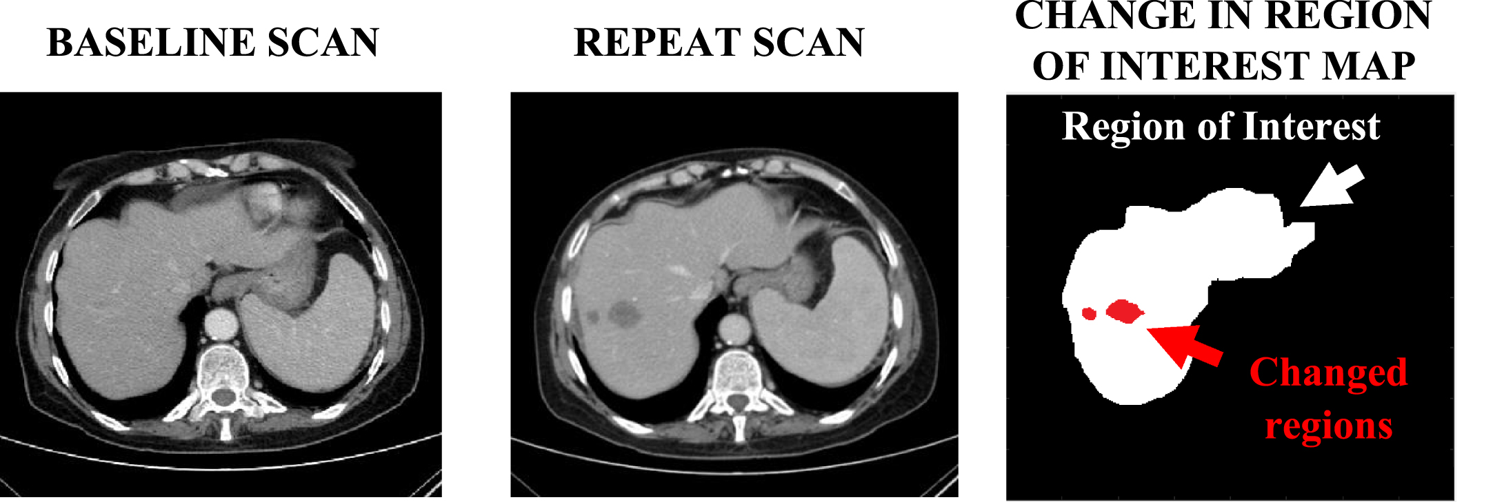
A Change in Region of Interest Map (CRIM) showing two liver lesions (arrow) that appear in the repeat scan but not in the baseline scan (window width = 350 HU, window level = 50 HU).

Differences between two scans may have been caused by clinically significant changes in the patient. However, differences can also be the result of patient repositioning and scan acquisition at different respiratory and cardiac stages. These non-rigid deformations are diagnostically irrelevant but may be mistaken for genuine changes. This ambiguity poses a challenge for radiologists examining scan pairs. Distinguishing between these two types of differences is thus a key challenge of automatic change detection in repeat CT scan studies.

CT scanning has the main drawback of exposing the patient to possibly harmful ionizing radiation [5]. This is exacerbated in repeat CT scanning, as the radiation exposure increases with each additional scan. The clinical indication for CT scan dose is described in the as low as reasonably achievable guidelines [6]. It is thus desirable to produce a CRIM for a repeat scan acquired with a reduced X-ray radiation dose.

Much research has been devoted to dose reduction in CT scanning. In this paper, we focus on dose reduction by sparse scanning, in which projection data is acquired during scanning from only a fraction of the scan angles. Using this approach, when only 10%of the scan angles are acquired, the patient is exposed to only 10%of the radiation dose. While sparse scanning is not yet implemented in commercial CT scanners, it could be achieved by alternating the voltage between 80–100 kV and 30–40 kV at different scan angles [7]. Standard reconstruction methods used with sparse scanning data yield streaking artifacts in the reconstructed image [8]. These artifacts greatly hinder change detection, as they add irrelevant changes and obscure genuine differences between the two scans.

The objective of this study is to accurately detect changes in a region of interest of a sparse-view repeat CT scan. The proposed method distinguishes between genuine changes and changes caused by non-rigid patient movement using very few scan angles. This increases the usefulness of sparse-view scans and allows clinicians to acquire such dose-reduced scans in additional clinical settings.

The innovation of the proposed method lies in the two challenges that it overcomes: it can detect changes even when the repeat scan is: (1) highly sparse and (2) contains non-rigid patient deformations. The challenge of high sparsity is overcome by performing the detection in Radon space without reconstructing the repeat scan image, thus bypassing the severe artifacts caused by sparse scanning. This also leads to short run times (minutes instead of hours). The challenge of non-rigid deformations is met using adaptive registration and detection methods tailored to the type of changes in the repeat scan, identified using a novel method for automatic estimation of the change properties.

2 Previous work

Changes can be detected in sparse repeat scans either in image space or in Radon space. In the image space approach, the repeat image is first reconstructed from the sparse projection data; the CRIM is then computed by comparing the two images. The Radon space approach computes the CRIM directly from the projection data without reconstructing the image.

The image space approach requires accurate reconstruction of the sparse CT scans. Many such reconstruction techniques have been developed. For example, Sidky and Pan [9] describe an iterative compressed sensing method in which the scan image is computed by minimizing its total variation subject to a fidelity constraint that requires that the acquired and computed image projections be similar. This method assumes that the image is piece-wise constant and may cause over-smoothing. Liu et al. [10] propose using an adaptive weighted total variation measure to avoid this effect.

The prior-image-based reconstruction (PIBR) approach uses data from a previous scan of the same patient to improve the dose-reduced image quality [1 , 12]. A prominent example of this approach is prior image constrained compressed sensing (PICCS) [1], in which a term in the objective function encourages similarity between the repeat scan image being reconstructed and the baseline image. PICCS produces high quality images when the two scans are aligned. Much research has been based on this method and expands on its general framework. Dang et al. [11] propose dPIRPLE, a deformable prior image registration, penalized likelihood estimation algorithm in which the optimization procedure simultaneously computes the image and performs non-rigid registration using a 3D B-spline-based deformation model. In the reconstruction of differences (RoD) method [12], the difference image between two scans is directly computed without reconstructing the repeat image. RoD assumes that the difference image is sparser than the repeat image and that it can be computed more accurately. RoD is limited to rigid transformations. PIBR methods produce better results than standalone techniques but may be less appropriate for image-based change detection: enforcing similarity between the two scans may cause small differences to be omitted from the reconstructed repeat scan, leading to missed changes in the CRIM. Note that this issue is not a concern in the Radon space approach, which does not require a reconstructed image.

Once the repeat image is reconstructed, the changed regions can in principle be located by image subtraction, as in digital subtraction angiography [13]. To avoid high false-positive rates, the differences caused by misalignment and genuine changes must be distinguished. For this purpose, advanced change detection methods have been developed for specific pathologies. For example, Ko and Betke [14] describe a method for automated lung nodule detection in follow-up CT scans; Vivanti et al. [15] present a method for liver tumor detection and tracking. These methods identify changed regions in the repeat scan and provide volumetric measurements of the changes. However, they assume that both scans were acquired at full dose and cannot handle reduced-dose imaging artifacts.

The Radon space change detection approach consists of computing the CRIM directly from the projection data by comparing the two scan sinograms. In previous work, we describe a method based on this approach [16]. First, the two scans are aligned using Radon space rigid registration. Rays crossing changed regions are detected and then back-projected, producing a likelihood map showing how many changed rays crossed each region of the image. The changed region map is then computed from the likelihood map. While our method is not constrained by a ROI, it is limited to rigid transformations.

Many Radon space non-rigid registration methods have been developed for sparse repeat CT scans. Zeng et al. [17] model deformations caused by respiratory motion using a B-spline transformation. Their method minimizes the difference between the repeat scan projections and the estimated projections of the transformed baseline image. Adelman and Joskowicz [18] define a similar cost function and model deformations with a deformation field whose control points are selected from edges in the baseline scan. Wang and Gu [19] align scans by first reconstructing a low-quality repeat image and performing image space registration. The computed deformation field is then used in the second stage as the initialization of Radon space registration.

In principle, Radon space change detection methods, and particularly ours [16], can be extended to handle non-rigid deformations by using one of the non-rigid registration methods listed above. However, existing Radon space change detection methods require a very accurate alignment of the two scans, which is achievable for rigid transformations but not for deformable ones. This limits the applicability of these methods to clinical scenarios in which the deformations are negligible, e.g., brain scans. Using them to detect changes in the chest or abdomen will lead to high false positive rates. Figure 2 illustrates this with examples of rigid and non-rigid registration results.

Fig. 2

Difference images following registration with rigid and non-rigid deformations. (a): clinical baseline scan (window width = 350 HU, window level = 50 HU); (b): simulated repeat scan obtained by applying a rigid transformation to the baseline scan; (c): the difference between (a) and the aligned repeat scan after rigid registration; (d): clinical repeat scan of the patient in (a) with non-rigid deformations. (e): the difference between (a) and the aligned repeat scan after non-rigid registration. The vertical bars show the HU display windows of the difference images.

In conclusion, the limitations of existing methods for change detection in the presence of non-rigid deformations include: 1) they may miss small or low contrast changes due to errors in the reconstruction of the repeat scan; 2) they are prone to high false-positive rates, mistakenly marking misaligned regions as changed; 3) they do not support high sparsity in the repeat scan since they require very high quality repeat scan images.

3 Materials and methods

We present next a new method for change detection in a ROI of a sparse repeat CT scan with non-rigid deformations, that produces an accurate CRIM as desired. It uses non-rigid Radon space registration and new techniques for distinguishing genuine differences from those caused by misalignment in the ROI. It significantly improves our previous Radon space method [16], which assumes that rigid registration yields a near-perfect alignment of the scans.

This Section is organized as follows. Subsection 3.1 presents the mathematical background and notations. Subsection 3.2 summarizes the change detection method for repeat scans with rigid deformations [16]. Subsection 3.3 presents the proposed method for repeat scans with non-rigid deformations.

3.1 Mathematical background and notations

For simplicity, we describe our method in the setting of parallel beam scanning; it is directly applicable to other scanning geometries, as discussed later. In parallel beam scanning, the scan acquisition is performed in a series of parallel planes (slices). In each plane, measurements from parallel rays are collected from indexed detectors evenly spaced on a line opposite the radiation source, at dense, evenly distributed angles. A scanning ray L on slice z with a coordinate system defined at its center is parameterized by the ray detector index s and the angle θ of the ray’s normal with the slice’s horizontal axis. The Radon transform of image F is a function $RF : ℝ \times [0^{\circ}, 179^{\circ}] \times ℕ \to ℝ$ such that: RF (s, θ, z) = ∫_L(s,θ,z) F (X) dμ, where X is a spatial coordinate vector and dμ is the standard measure on L (s, θ, z). A sinogram is a 2D matrix whose rows and columns are the scanning angles θ and the ray detector indices s, respectively, with values equaling the Radon transform at each angle and detector index. The sinogram scan stack is a 3D matrix formed by a stack of the sinograms of each image slice.

3.2 Change detection in scans with rigid deformations

For completeness, we summarize our Radon space change detection method for rigid transformations. The input is a previously acquired full dose baseline scan (image and sinogram), and a sparsely sampled repeat scan sinogram acquired at a subset of scan angles. The output is a changed region map –a 3D binary matrix indicating which voxels in the repeat scan image have changed. The method has four steps:

Rigid registration: the sparse repeat scan sinogram stack is rigidly registered to the full baseline scan sinogram stack in 3D Radon space with the method of [20].

Changed ray detection: for each angle θ and for each slice z, the rays which passed through changes are detected with the dynamic thresholding method in [7].

Likelihood map computation: for each slice z, the changed rays found in step 2 are back-projected onto image space. This yields a likelihood map showing how many changed rays crossed each pixel (voxel in slice z), indicating the likelihood of each pixel having been changed.

Changed region map computation: for each slice z, a greedy algorithm locates the changed regions in that slice based on the likelihood map from step 3. The changed region maps of each slice together form a 3D map.

Each step’s success crucially depends on that of the previous one. When the rigid registration in step 1 does not yield sub-millimetric alignment, many false positives will appear when detecting changed rays in step 2. These errors will be added to the likelihood map, leading to false positives in the changed region map in step 4. Consequently, merely replacing the rigid registration in step 1 with non-rigid registration will yield many spurious detected changes due to misalignment, thereby yielding an inaccurate changed region map.

3.3 Change detection with non-rigid deformations

The new method for change detection in a ROI of a sparse repeat scan with non-rigid deformations is based on our previous method, with several new steps and significant enhancements to existing stages with improved techniques.

The inputs are: 1) a previously acquired full baseline scan image and sinogram; 2) a sparsely sampled repeat scan sinogram, and; 3) a user-defined ROI that includes the organ of interest. The output is a CRIM –a binary matrix that indicates which of the voxels in the ROI of the repeat scan image have changed. The method consists of a pre-processing step followed by five steps (Fig. 3). For consistency with the previous method, the step numbers begin with 0). To simplify the algorithm’s description, the term ROI is used in this work to refer both to the entire 3D map indicating the volume of interest to the clinician, and to each 2D map indicating the clinically relevant regions in each slice.

Fig. 3

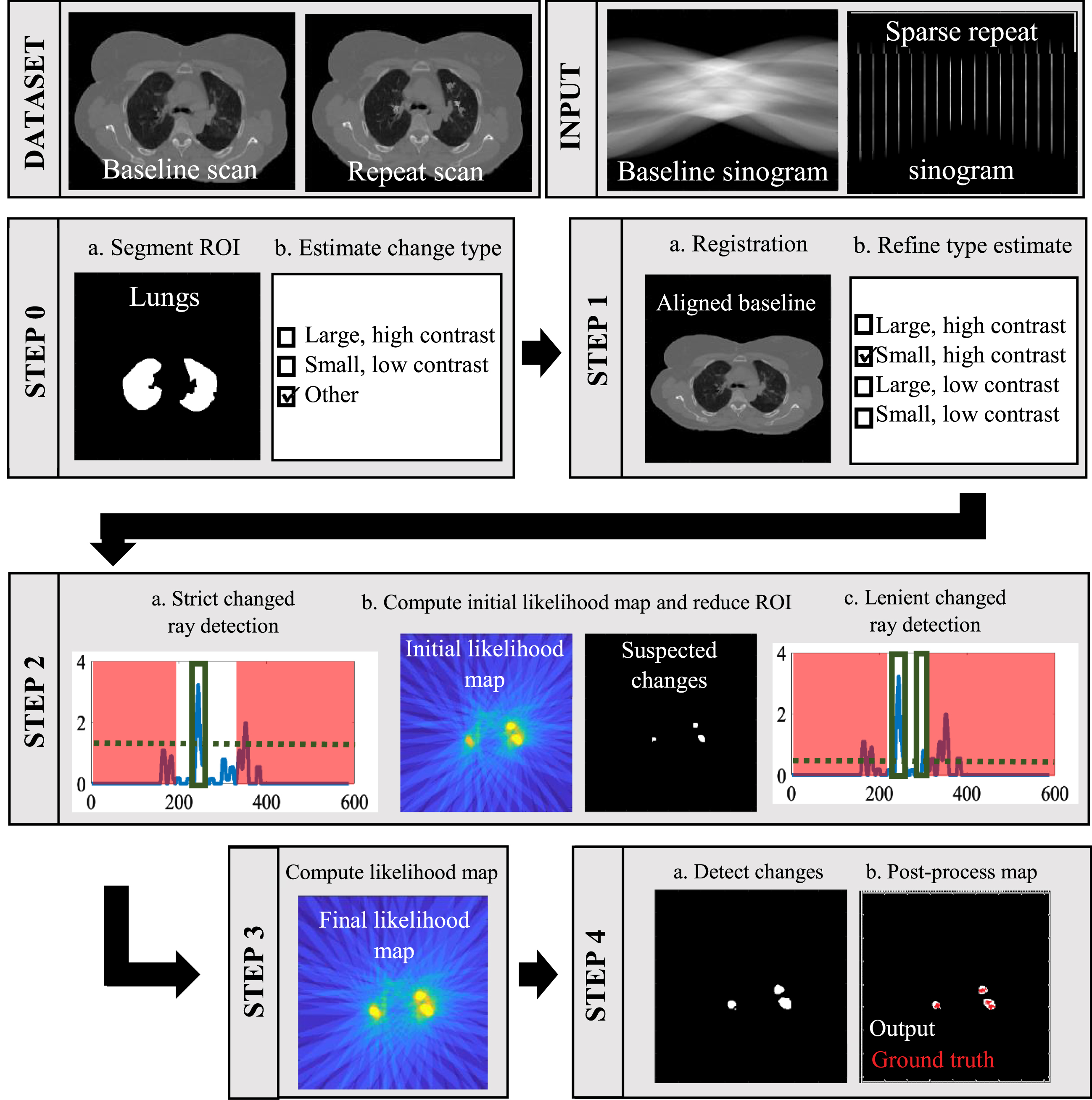
Illustration of the proposed change detection method, run on a pair of scans with simulated changes added to the repeat scan (top).

Pre-processing: Changed region properties:

ROI segmentation: the baseline scan image voxels belonging to the organ selected as the ROI are identified by automatic segmentation.

Estimation of changed region properties: the size and contrast of the differences between the two scans are categorized based on the difference between the unaligned scan sinograms.

Non-rigid registration:

Registration: The sparse repeat scan and the full baseline scan sinogram stacks are non-rigidly registered with the Radon space method in [18].

Final estimation of changed region properties: the classification in step 0.b is refined using the difference between the aligned sinograms.

Changed ray detection:

For each slice z:

Strict changed ray detection: for each angle θ, the rays that cross changed regions in the ROI are detected by thresholding. High threshold values are selected to produce a low false-positive rate.

ROI reduction: an initial change likelihood map is computed by back-projecting the detected changed rays onto image space. This likelihood map is used to locate regions in the ROI which are suspected to contain changes. The ROI is reduced to these suspicious regions.

Lenient changed ray detection: for each angle θ, the rays that cross changed regions in the reduced ROI are again detected using thresholding. This time, lower threshold values are selected to produce a low false-negative rate.

Likelihood map computation: for each slice z, the changed rays detected in steps 2.a,c are merged and back-projected onto image space. Each ray in the map is assigned a weight reflecting how much of the ray crossed the ROI.

Changed region map computation:

Changed region detection: the CRIM is computed from the likelihood map with the greedy algorithm described in [16]. The regions inside the ROI with high likelihood values are also added to the CRIM.

False positive removal: regions in the CRIM are evaluated and removed when they are deemed as false positives. The final CRIM is post-processed based on the estimated properties of the changed regions.

This method is directly applicable to cone beam scanning without re-binning the scan data to simulate parallel beam scanning. In the registration algorithm of [18] in step 1.a, the scanner system matrix in the objective function is replaced with one that represents cone beam scanning geometry. This reduces the method’s efficiency but does not affect its output. In steps 0.b, 1.b and 2, the change type estimation and the changed ray detection techniques make no assumption regarding the scan angle geometry. In step 3, the likelihood maps are computed by back-projecting the changed rays from all planes and adding the weight of each ray to all the voxels they cross in the likelihood map [16]. In step 4, the change detection algorithm proceeds with the new likelihood maps, as it does in the parallel beam case.

Next, we describe each stage of the algorithm in detail as follows.

3.3.1 ROI segmentation (step 0.a)

The ROI can be an organ or a body region and is chosen by the user in advance based on the clinical need. For example, if the purpose of the repeat scan is to track the growth of pulmonary tumors, the lungs are selected as the ROI. For the ROI segmentation, simple segmentation techniques, e.g., thresholding and edge detection suffice because the result need not be very accurate. The ROI segmentation can also be computed with any one of many existing techniques [21 –23].

3.3.2 Changed region property estimation (steps 0.b and 1.b)

To estimate the change properties, we characterize the changes in the repeat scan by their size and contrast level with respect to the baseline image. We define four types of changes: 1) large, high contrast changes; 2) small, high contrast changes; 3) large, low contrast changes; 4) small, low contrast changes.

Each type of changes appears differently in the difference between the sinograms of the repeat and baseline scans (Fig. 4). For large, high contrast changes, the baseline and repeat scan sinograms exhibit large differences that are detectable without registration. In contrast, small, low contrast changes yield small differences, often obscured by the scans’ misalignment. The sinogram difference will thus have very low values. Small, high contrast changes and large, low contrast changes have a similar range of values in the sinogram difference. However, large changes are crossed by more consecutive rays at each angle than small changes. This distinction appears in the aligned sinogram difference as longer segments of non-noise values in each column, which correspond to the consecutive changed rays.

Fig. 4

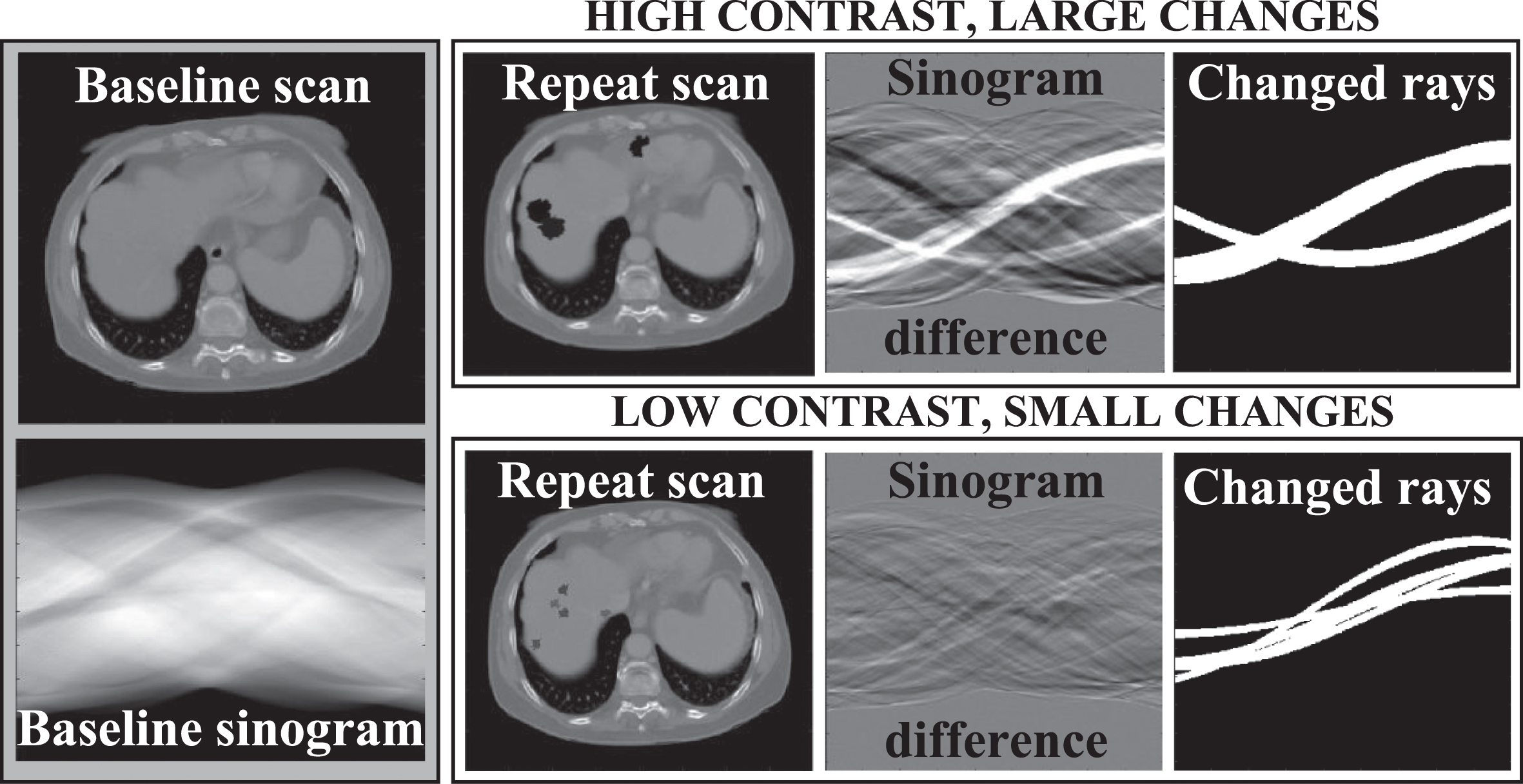
Typical sinogram difference images. Left: the baseline scan image and sinogram. For two types of changes, we show: the repeat scan with different simulated changes added to it (left, window width = 1500 HU, window level = 50 HU); the difference between the baseline and repeat sinograms (middle); pixels in the sinogram difference corresponding to rays crossing changed regions (right).

We propose a rule-based approach to distinguish between the different types of changes. Large, high contrast changes and small, low contrast changes (types 1 and 4) are identified using the unaligned sinogram difference in step 0.b. In step 1.b, the aligned sinogram difference is used to complete the procedure. In both steps, we compute features of the sinogram difference which reflect the extent of the changes between the two scans. These features are as follows:

H: The number of high values in the unaligned sinogram difference greater that a predefined threshold C_H (H = # values> t_H). High values indicate large changes.

NN: The number of non-noise values in the unaligned sinogram difference greater that a predefined threshold t_NN (NN = # values> t_NN, where t_H > t_NN). Low values indicate that there are no large changes. Large values indicate that there are large changes in at least one slice.

MM: The maximal mean value of the aligned sinogram difference of a single slice. Sinogram values corresponding to rays that do not cross the ROI are disregarded. (MM=max_z (mean (vals in slice z))).Large values indicate that there are large changes in at least one slice.

The classification procedure, described next, is summarized in Fig. 5.

Fig. 5

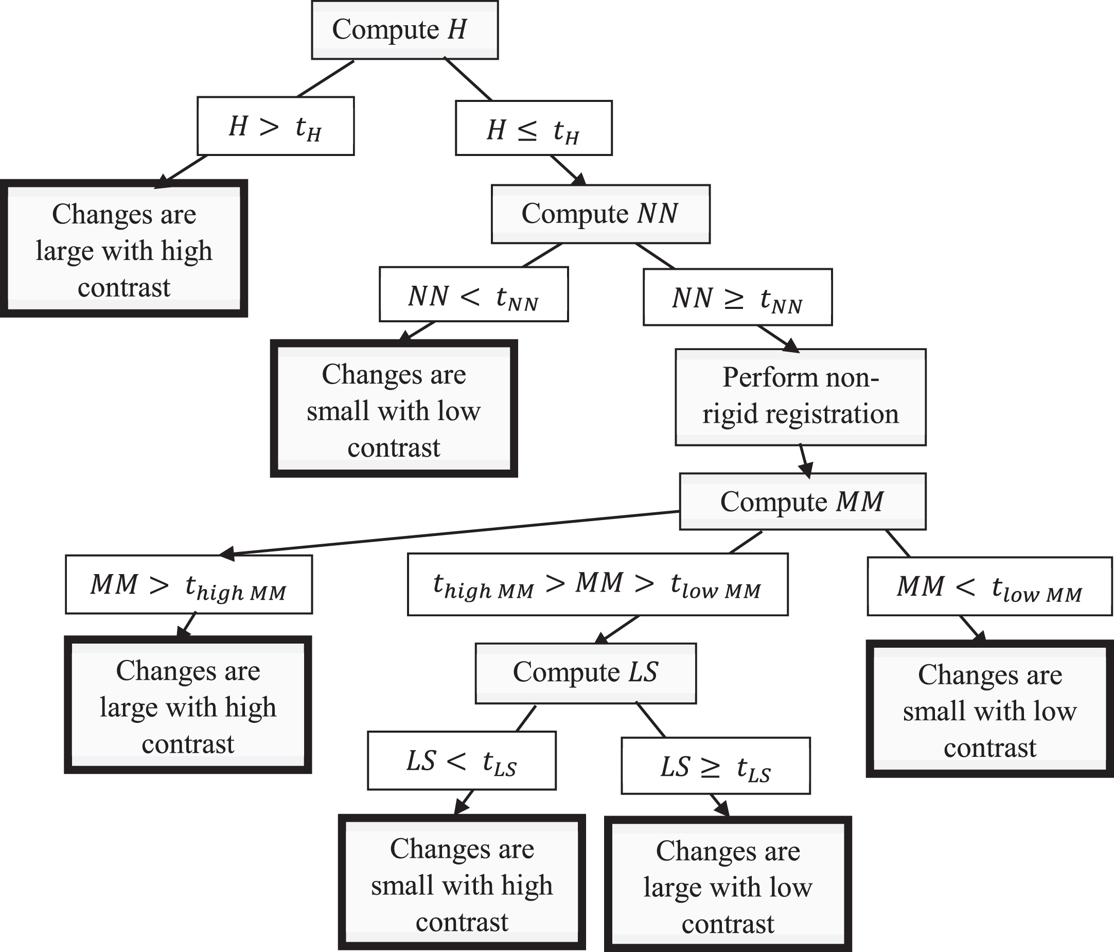
Flow chart describing the rule-based procedure for estimating the type of changes in the repeat scan in steps 0 and 1 of the algorithm.

LS: The number of entries belonging to long sequences (>15) of high values of predefined threshold c_LS high values (LS> c_LS) in columns of the aligned sinogram difference. Sinogram values corresponding to rays that do not cross the ROI are disregarded. High values of LS indicate large changes.

In step 0.b, we compute the number of high values (H) and the number of non-noise values (NN) in the unaligned sinogram difference. Next, we apply these rules:

The changes are large with high contrast if H > t_H

The changes are small with low contrast if H < t_H and NN < t_NN

In step 0.b, we compute the number of high values (H) and the number of non-noise values (NN) in the unaligned sinogram difference. Next, we apply these rules:

The changes are large with high contrast if H > t_H

The changes are small with low contrast if H < t_H and NN < t_NN

If neither of these rules apply, the classification is completed in step 1.b, after the scans are registered. In this step, we compute the aligned sinogram difference, and set values to zero if they correspond to rays which do not cross the ROI. We then compute two features of the aligned sinogram difference: the maximal mean sinogram difference, MM, and the number of values belonging to long segments, LS. We then apply these rules:

The changes are large with high contrast if MM > t_high MM

The changes are small with low contrast if MM > t_low MM

The changes are small with high contrast if t_low MM < MM < t_high MM and LS < t_LS

Otherwise, the changes are large with low contrast.

The values of the constants in steps 0.b and 1.b are chosen empirically based on the imaging properties of the selected organ in the ROI.

The classification is used in the next steps of the algorithm. Parameter values for the registration (step 1.a), the changed ray detection (step 3), and the changed region map computation (step 4) are selected based on the type of changes in the repeat scan. For example, the thresholds for adding high likelihood pixels to the CRIM (step 4.a) are set according to the change type. In step 4.b, the changed region map is post-processed according to the change type: medium sized regions are expanded when the changes are estimated to be large, and large regions are shrunk when the changes are estimated to be small.

Following the classification according to size and contrast of the changes, the MM value is used to estimate the extent of the misalignment between the two scans after the registration. High MM values indicate more significant misalignments while low MM values indicate better alignments. This estimate is also considered when setting the parameter values is later steps.

3.3.3 Non-rigid registration (step 1.a)

We use the 3D Radon space non-rigid registration algorithm in [18]. In this method, the transformation is modeled using a set of control points sampled randomly from the edges of the baseline image. The method computes the displacement vectors of the control points and interpolates the deformation field of the remaining voxels. The loss function is based on the difference between the repeat sinogram and the transformed baseline sinogram, and is minimized by gradient descent.

The number of control points and the gradient descent parameters are critical for the performance of this algorithm as they control which deformations can be applied to align the baseline and the repeat scans. Excessive deformations cause over-fitting and eliminate genuine differences; restricted deformations cause under-fitting and create spurious misalignment differences. The extent of the deformation is therefore controlled according to the type of changes. For large, high contrast changes, fewer control points and optimization iterations are used. For small, low contrast changes, more control points and optimization iterations are used. These cases are identified in step 0.b prior to the registration and appropriate parameter values are set accordingly. If one of these cases is identified only in step 1.b, after the scans were already registered using sub-optimal parameter values, the registration is repeated with the appropriate parameters.

3.3.4 Changed ray detection (step 2)

Changed rays are detected in three stages. First, changed rays in the aligned sinogram difference are detected using thresholding (step 2.a). The threshold value is defined adaptively based on the estimated types of changes in the repeat scan. A high threshold value is set to minimize false positives –rays with differences smaller than this threshold are not considered changed. The detected changed rays are back-projected to image space to create a partial likelihood map, indicating regions of the repeat scan which were crossed by many changed rays. This initial map is imprecise but allows the identification of regions inside the ROI which may contain changes. This map is processed as a 2D grayscale image (step 2.b). First, the map contrast is increased using a Gamma filter and the map is blurred with a Gaussian kernel. Then, pixels in the ROI with intensities that are local maxima are detected. These pixels constitute the reduced ROI. Changed rays which cross the reduced ROI and may have been missed in step 2.b are then detected using a lower threshold, thereby increasing the detection sensitivity in the targeted areas (step 2.c).

3.3.5 Likelihood map computation (step 3)

The likelihood map of each slice is a 2D matrix the size of the slice with values between 0 and 1. Each entry in the matrix represents the likelihood of the corresponding pixel in that slice belonging to a changed region. The likelihood map is computed using the following procedure. Each changed ray detected in step 2 is assigned a weight equaling the number of pixels in the ROI that the ray crosses. This weight reflects the confidence that changes detected in the ray were due to changes inside the ROI rather than changes outside it. The likelihood map for each slice is computed by back-projecting the slice’s changed rays onto image space. For each ray, the values in the map that correspond to pixels crossed by that ray are increased by the ray’s weight. The final value of each pixel is the sum of the weights of changed rays that crossed that pixel. Normalizing the values in the map yields the likelihood (probability) of each pixel having changed. Fig. 3 shows an example of a likelihood map (bottom-left).

3.3.6 Changed region map computation (step 4)

The initial changed region map is computed iteratively from the likelihood map with a greedy algorithm (step 4.a). In each iteration, pixels with the highest likelihood values are added to the map, then rays crossing the pixels already in the map are removed. This process continues until no changed ray intersections remain. The resulting map is expanded by computing the convex hulls of the sets of connected components in the map which cannot be separated by a line in the slice plane. Pixels with high likelihood map values are also added to the changed region map.

The final CRIM is obtained by removing regions and entire slices in the changed region map estimated to be false positives (step 4.b). In each CRIM slice, connected components that do not match the estimated change properties are removed, e.g., small regions are removed from scans estimated to contain large changes. Entire slices are evaluated based on the distribution of high values in the likelihood map. When true changes are found, the likelihood map typically contains a few well-defined regions with high likelihood values. Otherwise, there are typically either no high likelihood values, or many small, scattered regions with high likelihoods. We identify these cases using the maximal value of the likelihood map, the number of zeros in the likelihood map, and the number of connected components in the likelihood map with high values. Changed regions whose maximal value is too low, that have too many pixels with a value of zero, or whose number of connected components is too high are removed from the CRIM. The thresholds are chosen empirically based on the resulting CRIM quality. To compensate for also removing true changes from the map, we copy the remaining regions in each slice to adjacent slices in the CRIM.

4 Experiments and results

We implemented the new method, tested its performance on clinical lung and liver CT scan pairs, and compared it to existing change detection methods. Subsection 4.1 describes the datasets of the experiments. Subsection 4.2 describes the performance measures. Subsection 4.3 presents the new method’s results and describes the parameter value selection experiments. Subsection 4.4 compares the new method to three other methods.

4.1 Datasets

We obtained two sets of clinical scans from two different patients from the Hadassah University Medical Center (Jerusalem, Israel): four intra-operative lung CT scans and a pair of diagnostic liver CT scans. Each set consisted of scans of the same patient acquired at different times. The repeat scans include patient motion and anatomical deformations caused by breathing and physiological processes. The scans were cropped along the z axis to remove slices containing genuine changes.

The set of lung scans consists of four CT scans, each acquired a few minutes after the last, during a biopsy procedure. After cropping, each scan consists of 412×412×6 voxels with spatial resolution of 0.97×0.97×2.5 mm³. We paired the first scan with each of the other scans to generate three scan pairs. The liver scan study consists of two scans acquired several months apart to evaluate the patient’s disease progression. After cropping, each scan consists of 400×400×7 voxels with spatial resolution of 0.85×0.85×1.5 mm³. Both the lung and the liver scan images’ intensity values were normalized to the [0,1] range. The scans were coarsely aligned by standard image-based rigid registration. Following this basic alignment, it was sufficient to perform the Radon space non-rigid registration step on each slice separately in 2D rather than in 3D, shortening run-times.

To generate known and measurable ground-truth changes in the repeat scans, we computed new repeat scan images by adding artificial regions to the original repeat scan image that simulate the appearance of bleeds and tumors. The changes consist of pseudo-ellipsoids with non-uniform gray levels in the organ of interest, e.g. the lungs and the liver. The number, location, size, and mean gray levels of the changed regions were chosen randomly and independently for each repeat scan. Thus, the organ motion and changes of body position in the datasets were genuine, while the changed regions being detected by the algorithm were synthetic.

Following the methodology of our previous study [16], we define two size ranges: small (4–18 voxels, 3–17 mm) and large (22–40 voxels, 21–35 mm) in each dimension, and two contrast ranges: low (0.1–0.2) and high (0.25–0.5), equaling the difference between the mean intensity of the baseline and repeat CT scans in the changed region. The number of changed regions is 4–5 for small changes and 3–4 for large changes.

We generated 120 trial datasets using each scan pair, totaling 360 lung scan trials and 120 liver scan trials. Each trial consists of the original baseline scan image and its full sinogram stack, and of an augmented repeat scan image and its sparse sinogram stack. The full sinogram stack includes each slice’s sinogram with 180 scan angles (0°–179°); the sparse sinogram stack is composed of each slice’s sparse sinogram with 18 (10%) evenly spaced angles (0°, 10°, 20°, . . . 170°). The sinograms are computed as the line integrals of the slice at the specified angles. The repeat scan sinograms are computed following the augmentation of the repeat scan images, and thus contain the simulated changed regions. Electronic scanning noise was added to the repeat sinograms with the noise model of Žabić et al. [24]. We generated 30 augmented repeat scan images for each of the four size/contrast combinations, totaling 30×4 = 120 trials. The augmented images used in the experiments reported below were used just in the testing phase and were not previously seen while developing the algorithm.

In the lung trial datasets, the simulated changed regions have higher intensities in the repeat scan than in the baseline scan, e.g., bleeds and lung nodules surrounded by air [25]. In the liver trial datasets, changes have lower intensities, simulating hypodense liver tumors in non-contrast CT scans [26]. These properties are used as prior knowledge by all change detection methods. Radon space methods only considered positive/negative values in the sinogram difference as changes, depending on the scanned organ. The image space method only marked positive/negative values in the image difference as changed.

4.2 Performance measures

We quantify the accuracy of the CRIMs with the changed region recall: the %of correctly identified changed voxels out of all changed voxels. We measure the changed region recall for each changed region separately and for each scan as a whole. We define a missed change as a region with a recall s< 10%.

We quantify the output’s precision with the adjusted precision measure in [16], which reflects the clinical usefulness of the output. From a clinical perspective, a CRIM with slightly expanded changed regions is no less informative than a map with perfect precision. The standard precision measure penalized outputs of this sort and is therefore not appropriate for our purposes. The adjusted precision is similarly defined as the standard measure, but is computed with respect to an adjusted ground truth that includes voxels that the algorithm is allowed to mark as changed, even if they were not actually changed. The adjusted ground truth is computed by first adding a 3-pixel margin around each real changed region and then computing the convex hulls of each set of disjoint connected components. The adjusted changed region precision is defined as the %of voxels marked as changed in the output that were included in the adjusted ground truth. This measure allows us to add a small margin around the changed regions in the CRIM without reducing the precision and is less sensitive to the size of the changes than the standard precision measure.

4.3 Method performance

Table 1 summarizes the performance of the new change detection method on the lung and liver datasets. Figure 6 shows examples of inputs and outputs. The following two subsections describe these results in detail and the parameter value selection process.

Table 1
Results of the proposed method on datasets based on the three lung scan pairs and the liver scan pair

Lungs Liver

TYPE OF CHANGE Mean recall (%) Mean adjusted precision (%) Missed changes / total changed regions Mean recall (%) Mean adjusted precision (%) Missed changes / total changed regions

Large, high contrast 97.8 95.3 0/316 96.0 99.5 1/104

Small, high contrast 88.3 86.0 25/400 90.3 83.8 4/133

Large, low contrast 86.6 91.9 17/323 92.8 92.3 2/102

Small, low contrast 71.5 67.3 91/406 65.3 78.9 35/133

	Lungs	Liver
Large, high contrast	97.8	95.3	0/316	96.0	99.5	1/104
Small, high contrast	88.3	86.0	25/400	90.3	83.8	4/133
Large, low contrast	86.6	91.9	17/323	92.8	92.3	2/102
Small, low contrast	71.5	67.3	91/406	65.3	78.9	35/133

Fig. 6

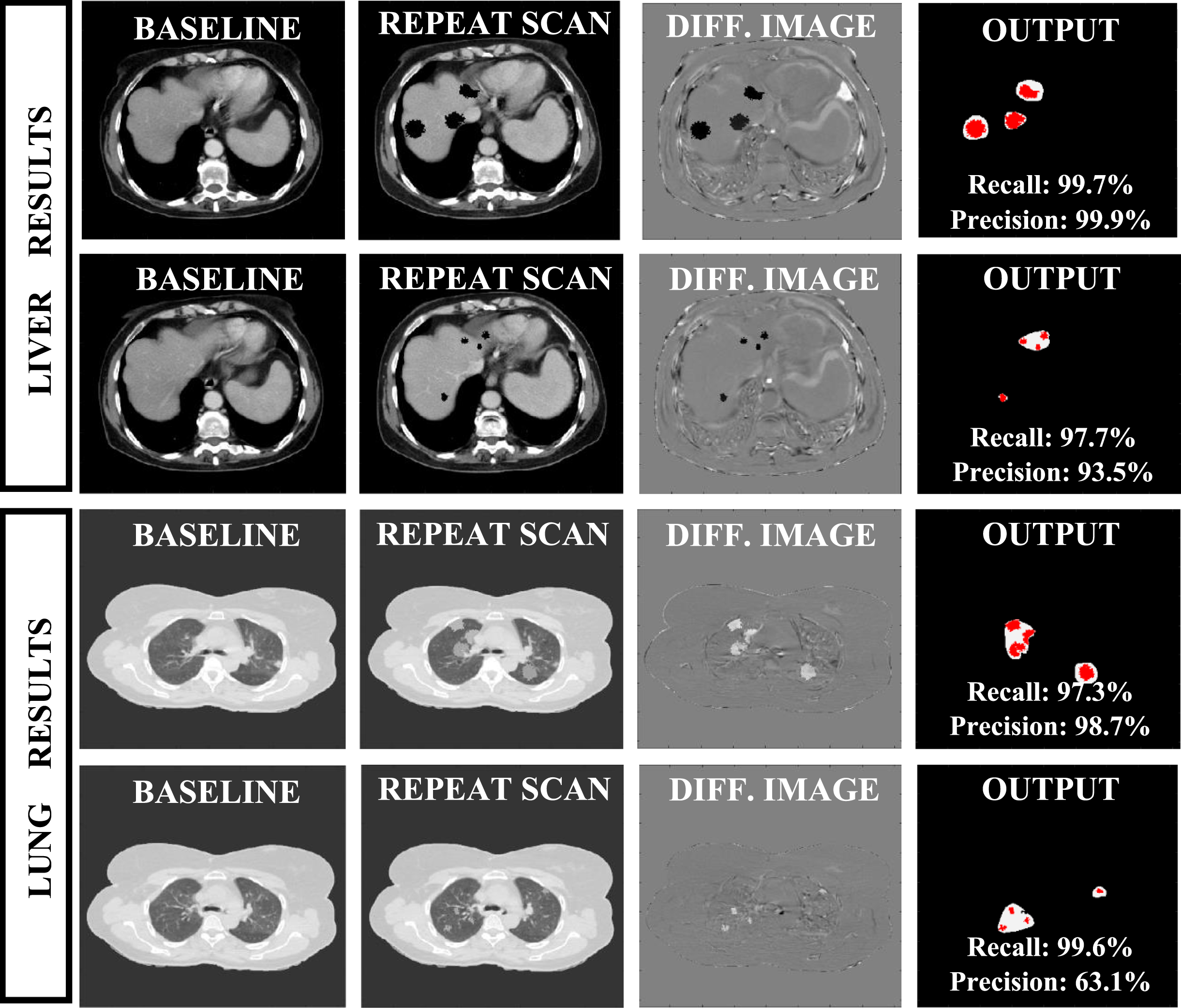
Examples of inputs and outputs of the proposed change detection method on the liver and lung datasets with simulated changed regions. Each row shows a different example. Two left columns: the baseline and repeat scan images (for liver scans: window width = 350 HU, window level = 50 HU; for lung scans: window width = 1500 HU, window level = –600 HU). Third column: the difference between the repeat image and the aligned baseline image, showing both the simulated changed regions and residual misalignment of the genuine patient scans which was not fully corrected in the registration step. Right column: the CRIM produced by the algorithm (white) and the ground truth (gray).

4.3.1 Performance on the lung and liver scan datasets

For the lung trials, the mean changed region recall rate of the new method is > 86%for all but small, low contrast changes. The precision rate for large tumors is > 91%, and for small, high contrast tumors is 86%. The recall rate for small, low contrast changes is lower, 71.5%. However, note that no slices with changes were missed. Results for the liver trials are comparable for high contrast changes (differences in recall and precision < 5%), and better for low contrast changes. In particular, the precision for small, low contrast changes was 78.9%for liver trials, compared to 67.3%for lung trials. Independent samples t-tests showed that the difference in performance for low contrast changes was significant (p < 0.005).

The changed region property estimation (steps 0.b and 1.b) yielded the following results. For the lung scan trials, only 16/360 cases were misclassified (<10%of the cases in each category). For the liver trial datasets, only 4/120 cases were misclassified.

4.3.2 Parameter value selection

The new method relies on various parameters that control its performance. Their values were chosen empirically based on extensive parameter selection experiments. In our previous work [16], we describe the methodology and experimental results used to select the number of scan angles and the parameter values for the greedy change detection method (step 4.a) for rigid deformations. The results are similar for the new method.

We describe next the experiments for the selection of the four main parameters of the change detection algorithm and discuss their effects on the output.

Non-rigid registration (step 1.a): the control point sampling rate and the maximum number of gradient descent iterations are two key parameters of the non-rigid registration method [18]. Since the size and contrast levels of the changes in the repeat scan image also affect the registration, the values of these two parameters are set separately for each type of changes.

We conducted a total of 7,680 (8×6×4×40) non-rigid registration tests on randomly generated 2D lung trial datasets to find the parameter values for each type of changes. We selected 8 sampling rates (1/5–1/70) and 6 maximum numbers of iterations (5–75).

Each combination of values was used to register a pair of slices. For each of the four types of changes, we repeated the experiment 40 times. The entire experiment was repeated on pairs of slices from each of the three lung scan pairs. A similar experiment was run using slices from the liver scan pair.

The true deformations between the baseline and repeat scans are unknown, as the scans were acquired in a clinical setting. However, following the registration, we expect the differences between the sinograms to be caused only by the simulated changes added to the repeat scan image. Consequently, we measure the registration quality by comparing the sinogram difference after the registration with the Radon transform of the simulated changes. The optimal parameter values are those that minimize the root mean square error between them.

For the lung scans, this experiment indicated that for high contrast changes, increasing the sampling rate causes over-fitting when using > 50 iterations, increasing the error. With fewer iterations, the error is not affected by the sampling rate. For small, low contrast changes, increasing the sampling rate increased the error, as in the high contrast case. The results for the liver scans showed different effects: for small changes, both increasing the number of iterations and increasing the sampling rate reduced the registration error.

Changed ray detection parameters (step 2): two thresholds are used to filter out differences between the aligned baseline and repeat sinograms that are too small to be considered changes. The threshold values are different for each type of change.

We conducted separate experiments to select the values of the two thresholds. The experiments were repeated for each type of change. The first stage of the changed ray detection identifies suspected changed regions. We therefore select its threshold based on the precision and recall of the map of suspected changed regions. In total, we tested 400 different cases: five threshold values on 20 different cases (individual slices) for each of the four change types. We repeated the experiment for each of the three lung scan pairs and for the liver scan pair. As expected, the higher the threshold, the higher the precision and the lower the recall of the suspected changed region map. Values were chosen to balance out the recall and the precision, with more weight given to the recall to avoid missing changed regions. The values of the second threshold were set by fixing the first threshold values and selecting the second threshold values based on the precision and recall of the final output. We tested an additional 320 cases for each scan pair. As in the first experiment, the higher the threshold, the lower the recall and the higher the precision.

4.4 Comparison with other change detection methods

We compare the new method’s performance on the first lung scan pair with three other methods: 1) our Radon space method for rigid deformations, using non-rigid registration instead of rigid registration [16]; 2) our new method using 3D Radon rigid registration; 3) image space change detection using a PICCS repeat scan reconstruction [1]. Table 2 summarizes the results.

Table 2
Results of four change detection methods on datasets based on the first lung contrast levels. The first row shows results of the proposed method. The second row shows results of the previous Radon space method using non-rigid registration. The third row shows results of the proposed method when using rigid registration instead of non-rigid registration. The last row shows results of the PICCS-based image space method

TYPE OF CHANGE MEASURE Proposed method, non-rigid reg. Previous method Proposed method, rigid reg. Image space method

Large, high contrast Recall (%) 99.8 81.1 99.7 96.3

Adjusted precision (%) 91.3 82.9 90.0 94.3

Missed changes / total changed regions 0/105 0/109 0/108 0/105

Small, high contrast Recall (%) 91.0 86.4 64.1 89.4

Adjusted precision (%) 84.9 58.0 86.1 89.6

Missed changes / total changed regions 4/134 5/130 36/142 5/138

Large, low contrast Recall (%) 95.9 92.2 72.3 88.1

Adjusted precision (%) 94.1 82.1 94.8 98.3

Missed changes / total changed regions 0/105 0/98 15/103 3/102

Small, low contrast Recall (%) 85.0 62.3 31.4 15.8

Adjusted precision (%) 67.8 35.3 52.6 94.7

Missed changes / total changed regions 12/135 25/137 80/136 97/135

TYPE OF CHANGE	MEASURE	Proposed method, non-rigid reg.	Previous method	Proposed method, rigid reg.	Image space method
Large, high contrast	Recall (%)	99.8	81.1	99.7	96.3
	Adjusted precision (%)	91.3	82.9	90.0	94.3
	Missed changes / total changed regions	0/105	0/109	0/108	0/105
Small, high contrast	Recall (%)	91.0	86.4	64.1	89.4
	Adjusted precision (%)	84.9	58.0	86.1	89.6
	Missed changes / total changed regions	4/134	5/130	36/142	5/138
Large, low contrast	Recall (%)	95.9	92.2	72.3	88.1
	Adjusted precision (%)	94.1	82.1	94.8	98.3
	Missed changes / total changed regions	0/105	0/98	15/103	3/102
Small, low contrast	Recall (%)	85.0	62.3	31.4	15.8
	Adjusted precision (%)	67.8	35.3	52.6	94.7
	Missed changes / total changed regions	12/135	25/137	80/136	97/135

4.4.1 Previous method with non-rigid registration

We compared the proposed method with our previous Radon space change detection method [16] described in Subsection 3.2. To adjust the previous method to the setting of repeat scans with non-rigid deformations, we replace the rigid registration algorithm in our Radon space change detection method [16] with the non-rigid registration algorithm in [18]. To allow a direct comparison with the new method, we also added an additional step in which we segment the organ of interest (lungs) and remove regions outside the ROI from the changed region map.

The previous method yields recall rates > 80%for all but small, low contrast changes, but has precision < 60%for small changes. For small, low contrast changes, an average of 11 false positive changed regions were detected in each slice, leading to a precision rate of 35%. For all types of changes, the previous method yields lower recall and precision rates than the new method. For small, low contrast changes, the difference is > 20%. Independent samples t-tests for each category of changes showed that the improvement in performance is statistically significant (p < 0.01) for all sizes and scan pair. This shows that using non-rigid registration does not suffice to compute an accurate CRIM in the presence of non-rigid deformations.

4.4.2 New method with rigid registration

We replace the non-rigid registration algorithm in the proposed method with the rigid registration algorithm in [20]. The results show that the new method successfully detects large, high contrast changes even with a rigid deformation model (recall = 99.7%, precision = 90.0%). However, the performance for other change types is much worse. Particularly, for small, low contrast changes the recall and precision are > 50%and > 15%lower respectively than with non-rigid registration. The classification in step 1.b is based on the aligned sinogram difference. Since the rigid registration is less accurate, this step fails: 68 out of 90 cases (75%) were misclassified as having large, high contrast changes because of alignment errors. This significantly reduced the performance in these cases. Independent samples t-tests showed that while the difference in the methods’ precision was not statistically significant, the recall rates were significantly higher (p < 0.0001) when using non-rigid registration. This demonstrates the importance of using a more accurate deformation model.

4.4.3 Image space change detection method using PICCS

To demonstrate the advantages of change detection in Radon space rather than in image space, we implemented a method which detects changes in the repeat scan by comparing the baseline image to a high-quality reconstruction of the sparse repeat scan. The first step consists of aligning the baseline and repeat scans using the same 3D Radon space non-rigid registration algorithm [18]. The sparsely sampled repeat scan is reconstructed with the PICCS algorithm [1], using the aligned baseline image as the prior. Next, the difference between the PICCS reconstruction and the aligned baseline image is computed, and the changed regions are identified with a preset threshold. Morphological operators are applied to refine the changed region map. Finally, the ROI selected by the user is segmented in the aligned baseline scan, and regions outside the ROI are removed from the map.

We performed a parameter selection experiment to select the parameter values for the PICCS algorithm. Each combination of parameter values that was tested was used to reconstruct the same 2D repeat scan image, using the same registered baseline scan as the prior. The repeat scan image included simulated small, high contrast changes. The PICCS reconstruction was compared to a full dose reconstruction of the repeat scan image computed using filtered back projection. The error was measured using the relative root mean square error (rRMSE) in a region of interest that includes the changed regions. To ensure robustness, we repeated the experiment with five different simulated scan pairs. We obtained the same set of optimal parameter values for all runs. In addition, the threshold used to detect the changed regions was chosen to be the lowest contrast level of changed regions in the simulated datasets. This ensured that all changes could potentially be detected while minimizing the false positive rate.

The image space method was successful for all but small, low contrast changes, with mean recall and precision rates comparable to those of the proposed Radon space method. The PICCS-based method yielded recall rates < 8%lower than the proposed method and precision rates < 5%higher. However, the PICCS-based method failed to detect most small, low contrast changes: the mean recall rate was only 15.8%, missing 97 out of 135 changes. The performance of the image space method in this case was significantly worse than that of the proposed method (p < 0.0001). The run time of the image space method was also > 10x longer than that of the proposed method –∼25 vs ∼2 mins when run on a 3D lung scan pair.

5 Discussion

Our results indicate that our method successfully detects nearly all changes for the lung and liver trial datasets: the changed region recall of the new method for all but small, low contrast changes is > 86%for lung scans and > 90%for liver scans. Over 90%of all changed regions were successfully detected in both the lung and liver scan pairs (>95%excluding small, low contrast changes). In contrast, our previous method performs much worse, particularly for small changes (precision < 60%, over 25%less than the proposed method). This indicates that even when replacing rigid registration with non-rigid registration, our previous method may not distinguish between genuine changes and differences caused by misalignment. Finally, our new method outperforms the image space PICCS-based method when detecting small, low contrast changes. The image space method misses×8 more small, low contrast changed regions than the proposed method. This shows the advantage of the Radon space approach over the image-based approach for sparse repeat scan change detection.

Our results also indicate that change detection in sparse repeat CT scans with non-rigid deformations is significantly more challenging than with only rigid deformations. It not only requires performing non-rigid registration in Radon space: it requires the additional estimation of the changed region properties and an advanced changed ray detection method. Without the distinction between the different change types, the registration either over-fits and obscures high contrast changes, or is not sufficiently precise to enable the detection of low contrast changes. It is also unable to optimize the balance between recall and precision individually for each change type.

The results reported above were obtained using only 18 scan angles. This shows that change detection is possible using ∼10%of a full dose scan of 180 scan angles, even in the presence of significant non-rigid deformations. The reduction in scan angles can yield a 10-fold reduction in radiation dose [10, 28], a significantly higher reduction than existing change detection methods. The new method can also be used to enhance existing dose reduction methods with a change detection component. For instance, the dose optimization algorithm in [7] reduces the dose by first detecting changed regions in Radon space and then scanning only the changed regions. Our method can also be used in conjunction with interior tomography methods, which reconstruct only a region of interest at full quality [28].

The novelties of our method are: 1) it accurately detects changes in a region of interest of a highly sparse repeat CT scan with non-rigid deformations, even when the changes are small with low contrast; 2) it adaptively registers the scans and detects changes based on the type of changes in the repeat scan, using a novel method for automatic estimation of the change properties; 3) it supports significant dose reductions in the repeat scan by sparse scanning; 4) it has short run times (minutes) since it does not reconstruct the repeat scan image.

Our new method shares several of our previous method’s advantages over other low dose change detection approaches [16]. Using a few, high mA projections rather than a full-view scan with lower tube currents facilitates the detection of subtle changes which may be obscured by noise in low mA scanning, while significantly reducing the patient’s exposure to radiation. Similarly, detecting changes in Radon space rather than in image space obviates compensating for reconstruction artifacts in the low dose image. Our results show that small, low contrast changes in the repeat image may be missed by advanced sparse-view reconstruction techniques such as PICCS [1].

Our new method greatly widens the practical applicability of the Radon space change detection approach in sparse repeat CT scanning. The previous method is limited to scenarios in which rigid registration suffices, e.g., brain and bone scans. Our results show that the new method is applicable to lung and liver scans, which include different types of deformations. The deformations in the liver scans are much larger than those in the lung scans, as much more time passed between the two scans’ acquisition. In the lung scans, the small bronchial structures are difficult to align, causing misalignment in the ROI. Our method robustly yields accurate results in both cases.

Finally, the CRIM produced by our method has many possible applications. It can save the clinician time by bringing his attention to subtle, clinically significant changes in the repeat scan which may have otherwise been missed, even in the presence of imaging artifacts caused by low-dose acquisition. It may also be used to reduce the patient’s exposure to radiation: a CRIM showing no significant changed regions can obviate the need for a full dose scan. On the other hand, a CRIM showing changes which are not visible in the low-dose reconstructed image may indicate that a full dose scan is necessary, but only for the slices containing changes.

Method limitations: Our new method shares some of the limitations of the previous Radon space method, which are discussed at length in [16]. Firstly, both change detection methods are limited by the intrinsic geometric properties of tomographic scanning. For example, they cannot distinguish between a ring-shaped change and a circular change of the same size because the changed rays in both cases are the same. Additionally, like the previous method, the new method produces a changed region map, not a scan image. If changes are detected in the repeat scan, a high-quality image may be needed to interpret them. However, by combining our method with the dose optimization method in [7], high quality, dose-reduced images can be generated by scanning only the changed regions. The interior tomography method in [17] can also be used to produce a high-quality reconstruction of those changed regions. The determination whether the high-quality scan image is necessary can be made automatically, and the patient can be re-scanned immediately following the initial sparse scan according to the locations of the detected changes.

The proposed method does not always detect all small, low contrast changes, because these changes are similar in both size and contrast to differences caused by the misalignment of the two scans. A more accurate non-rigid registration method may improve the detection rate for this type of change.

Another limitation of the proposed method is that it relies on several parameters whose values must be selected empirically. The appropriate values depend on the specific application and scan protocol. Our results show that despite this, the method is robust and succeeds on different scan pairs with different types of changes. Furthermore, the parameters have well understood, direct effects on the output, which simplifies the selection process and allows the user to control the method’s sensitivity.

Study limitations: our experimental studies quantify the performance of our method on repeat scans with simulated changes. Note however, that while the changed regions were added manually, the non-rigid deformations in the repeat scans were caused by genuine repositioning and movement of the patients. Using simulated changes allowed us to test many more test cases that would have been possible otherwise, more effectively demonstrating the robustness of our method.

A second limitation of our studies is that only one liver scan pair was used as the seed for generating the baseline and repeat liver scans. However, the changed regions in each trial were different, and the baseline scan was aligned differently in each case, adding variability to the inputs we tested. Furthermore, we tested the proposed method on inputs generated using three lung scan pairs in addition to the liver scan pair, demonstrating the method’s robustness.

6 Conclusion

We have presented a new change detection method for highly sparse repeat CT scans with significant, non-rigid deformations. It improves upon our previous method [16] and widens its applicability. It incorporates non-rigid registration in Radon space and a new method for distinguishing genuine differences in the ROI from those caused by misalignment using the changed region properties. The new method is automatic, accurate and robust. Our studies show that it successfully generates a reliable changed region map for both lung and liver scans, using only 10%of the full 180 scan angles. It outperforms both the previous Radon space change detection method and an image space thresholding method.

Our results demonstrate the feasibility of change detection in the presence of non-rigid deformations and indicate that the proposed method has potential clinical usefulness in many cases. A CRIM can streamline the radiologist’s work, indicating regions of interest. It can prevent changes from being over-looked and help reduce a patient’s overall radiation dose. In the future, we plan to further validate the method on pairs of patient scans with real changes.

Footnotes

Acknowledgments

This work was supported by the Israel Innovation Authority, Grant No. 57706.

Conflict of interest

None of the authors have any conflict of interest. The authors have no personal financial or institutional interest in any of the materials, software or devices described in this article.

Protection of human and animal rights statement

No animals or humans were involved in this research. All scans were anonymized before delivery to the researchers.

Presentation at conferences

The research described in this paper has not been presented in any conference to date.

References

Chen

G.H.

, Tang

and Leng

, Prior Image Constrained Compressed Sensing (PICCS): a method to accurately reconstruct dynamic CT images from highly undersampled projection data sets, Medical Physics 35(2) (2008), 660–663.

Zhao

, James

L.P.

, Moskowitz

C.S.

, et al., Evaluating variability in tumor measurements from same-day repeat CT scans of patients with non-small cell lung cancer, Radiology 252(1) (2009), 263–271.

Werner-Wasik

, Xiao

, Pequignot

, et al., Assessment of lung cancer response after nonoperative therapy: tumor diameter, bidimensional product, and volume. A serial CT scan-based study, International Journal of Radiation Oncology 51(1) (2001), 56–61.

Cleary

and Peters

T.M.

, Image-guided interventions: technology review and clinical applications, Annual Review of Biomedical Engineering 12 (2010), 119–142.

Davies

H.E.

, Wathen

C.G.

and Gleeson

F.V.

, The risks of radiation exposure related to diagnostic imaging and how to minimize them, BMJ Journal 342 (2011), d947.

McCollough

C.H.

, Bruesewitz

M.R.

and Kofler

J.M.

, CT dose reduction and dose management tools: Overview of available options, Radiographics 26(2) (2006), 503–512.

Shamul

and Joskowicz

, Radon space dose optimization in repeat CT scanning, –, IEEE Transactions on Medical Imaging 36(12) (2017), 2436–2448.

Crawford

C.R.

and Kak

A.C.

, Aliasing artifacts in computerized tomography, Applied Optics 18(21) (1979), 3704–3711.

Sidky

E.Y.

and Pan

, Image reconstruction in circular cone-beam computed tomography by constrained total-variation minimization, Physics Medicine and Biology 53(17) (2008), 4777–4807.

10.

Liu

, Ma

, Fan

, et al., Adaptive-weighted total variation minimization for sparse data toward low-dose X-ray computed tomography image reconstruction, Physics in Medicine and Biology 57(23) (2012), 7923–7956.

11.

Dang

, Wang

A.S.

, Sussman

M.S.

, et al., dPIRPLE: a joint estimation framework for deformable registration and penalized-likelihood CT image reconstruction using prior images, Physics in Medicine and Biology 59(17) (2014), 4799–4826.

12.

Pourmorteza

, Dang

, Siewerdsen

J.H.

, et al., Reconstruction of difference in sequential CT studies using penalized likelihood estimation, Physics in Medicine and Biology 61(5) (2016), 1986–2002.

13.

Brody

W.R.

, Digital subtraction angiography, –, IEEE Transactions on Nuclear Science 29(3) (1982), 1176–1180.

14.

J.P.

and Betke

, Chest CT: automated nodule detection and assessment of change over time –preliminary experience, Radiology 218(1) (2001), 267–273.

15.

Vivanti

, Szeskin

, Joskowicz

, et al., Automatic detection of new tumors and tumor burden evaluation in longitudinal liver CT scan studies, International Journal of Computer-Aided Radiology and Surgery 12(11) (2017), 1945–1957.

16.

Shamul

and Joskowicz

, Automatic change detection in sparse repeat CT scanning, IEEE Transactions on Medical Imaging 39(1) (2020), 48–61.

17.

Zeng

, Fessler

J.A.

and Balter

J.M.

, Estimating 3-D respiratory motion from orbiting views by tomographic image registration, IEEE Transactions on Medical Imaging 26(2) (2007), 153–63.

18.

Adelman

and Joskowicz

, Deformable registration and region-of-interest image reconstruction in sparse repeat CT scanning, –, Journal of X-ray Science and Technology 28(6) (2020), 1069–1089.

19.

Wang

and Gu

, High-quality four-dimensional cone-beam CT by deforming prior images, Physics in Medicine and Biology 58(2) (2012), 231–46.

20.

Medan

, Shamul

and Joskowicz

, Sparse 3D Radon space rigid registration of CT scans: method and validation study, IEEE Transactions on Medical Imaging 36(2) (2017), 497–506.

21.

De Nunzio

, Tommasi

, Agrusti

, et al., Automatic lung segmentation in CT images with accurate handling of the hilar region, Journal of Digital Imaging 24(1) (2011), 11–27.

22.

Heimann

, Van Ginneken

M.A.

, et al., Comparison and evaluation of methods for liver segmentation from CT datasets, IEEE Transactions on Medical Imaging 28(8) (2009), 1251–1265.

23.

, Hoffman

E.A.

and Reinhardt

J.M.

, Automatic lung segmentation for accurate quantitation of volumetric X-ray CT images, IEEE Transactions on Medical Imaging 20(6) (2001), 490–498.

24.

Žabić

, Wang

, Morton

and Brown

K.M.

, A low dose simulation tool for CT systems with energy integrating detectors, Medical Physics 40(2) (2013), 031102.

25.

Eguchi

, Yoshizawa

, Kawakami

, et al., Tumor size and computed tomography attenuation of pulmonary pure ground-glass nodules are useful for predicting pathological invasiveness, PloS One 9(5) (2014), e97867.

26.

Yoshimura

, Murakami

and Kim

, Angiomyolipoma of the liver with least amount of fat component: imaging features of CT, MR, and angiography, Abdominal Imaging, 27(2) (2002), 184–187.

27.

and Wang

, Compressed sensing based interior tomography, Physics in Medicine and Biology 54(9) (2009), 2791.

28.

Huang

, Zhang

, Ma

, et al., Iterative image reconstruction for sparse-view CT using normal-dose image induced total variation prior, PloS One 8(11) (2013), e79709.