Parameter tuning in machine learning based on radiomics biomarkers of lung cancer

Abstract

BACKGROUND:

Lung cancer is one of the most common cancers, and early diagnosis and intervention can improve cancer cure rate.

OBJECTIVE:

To improve predictive performance of radiomics features for lung cancer by tuning the machine learning model parameters.

METHODS:

Using a dataset involving 263 cases (125 benign and 138 malignant) acquired from our hospital, each classifier model is trained and tested using 237 and 26 cases, respectively. We initially extract 867 radiomics features of CT images for model development and then test 10 feature selections and 7 models to determine the best method. We further tune the parameter of the final model to reach the best performance. The adjusted final model is then validated using 224 cases acquired from Lung Image Database Consortium (LIDC) dataset (64 benign and 160 malignant) with the same set of selected radiomics features.

RESULTS:

During model development, the feature selection via concave minimization method show the best performance of area under ROC curve (AUC = 0.765), followed by l0-norm regularization (AUC = 0.741) and Fisher discrimination criterion (AUC = 0.734). Support vector machine (SVM) and random forest (RF) are the top two machine learning algorithms showing the best performance (AUC = 0.765 and 0.734, respectively), using by the default parameter. After parameter tuning, SVM with linear kernel achieves the best performance (AUC = 0.837), whereas the best tuned RF with the number of trees is 510 and yields a slightly lower performance (AUC = 0.775) in 26 test samples data. During model validation, the SVM and RF models yield AUC = 0.78 and 0.77, respectively.

CONCLUSION:

Appropriate quantitative radiomics features and accurate parameters can improve the model’s performance to predict lung cancer.

Keywords

Lung neoplasms machine learning radiomics parameter analysis lung nodule classification

1 Introduction

In recent years, radiomics has been proposed for diagnosis [1 –3]. It extracts a mass of textures and statistical information from medical imaging data, then uses feature selection to obtain the most valuable features for classification. Based on selected features, radiomics builds a machine learning model and then trains the model to classify and analyze medical data. Radiomics can help doctors diagnose patients more accurately, identify patients’ clinical status, and predict patients’ conditions [4]. Bodalal et al. provided a general review of radiogenomic literature concerning prominent mutations across different tumor datasets [5]. The radiomics features have potentially critical translational implications for identifying highly vulnerable non-small cell lung cancer (NSCLC) patients treated with immunotherapy [6, 7].

Feng proposed a radiomics nomogram used in preoperative differentiation between the minimally invasive adenocarcinoma (MIA) and invasive adenocarcinoma (IAC) in patients with sub-solid pulmonary nodules [8]. Some researchers discriminated adenocarcinoma in situ (AIS) and minimally invasive adenocarcinoma (MIA) from invasive Adenocarcinoma (IA) using radiomics features [9]. Radiomics features might harbor potential surrogate biomarkers for the identification of EGRF mutation statuses [10]. Jia’s method showed that radiomics could reflect the genetic differences between tumors and have diagnostic value and the potential to be a diagnostic tool [11]. Wang verified the efficiency of the radiomics model on computed tomography (CT) images of intratumorally and peritumoral lung parenchyma to predict the preoperative lymph node (LN) metastasis in patients with clinical stage T1 peripheral lung adenocarcinoma [12]. These studies suggest that radiomics could reveal tumor characteristics and thus be a helpful tool for oncologists.

Lung cancer is one of the most common cancers [1], and early diagnosis and intervention can improve the cure rate. Radiomics has been used in the diagnosis of lung cancer. It filters out some quantitative features and characteristics from image data. The elements reflect the molecular markers (radiogenetics) and heterogeneity of tumors, which are significant for identifying benign or malignant tumors and tumor development stage. The correlation between characteristic information and tumor data can be found by analyzing individual features and characterization [13 –15]. Overfitting is a significant issue in conventional radiomics. Many radiomics features are directly used to train and test models that can predict genotypes and clinical outcomes. Many features are redundant, and redundant features could mislead machine learning algorithms. Therefore, selecting practical radiomics features can improve the performance of the model. It is vital to remove redundant and irrelevant features before evaluating algorithms [16 –18]. Akihiro analyzed the standardization of radiomics parts. Peeken showed a predictive value for CT-based radiomics features in STS despite CT’s low soft-tissue contrast. Their machine learning models showed predictive performances for patients’ overall survival (OS), distant progression-free survival (DFPS), and local progression-free survival (LPFS) [20]. Quantitative radiomics features provide additional information over clinically-assessed qualitative features for differentiating invasive pulmonary adenocarcinomas (IPAs) from non-IPAs appearing as ground-glass nodules (GGNs) [21]. Numerous researchers presented feature extraction and parameter tuning approaches to improve the classification performance of machine learning, which has been effectively applied in other medical imaging fields [22 –26]. Only a few recent studies have compared different radiomics feature selection and classification models [27, 28].

This paper compared the diagnostic performance of different radiomics feature selection methods and parameter tuning for the classification algorithms. We investigated a machine learning model with parameter tuning in the multi-center dataset. We found that quantitative radiomic features extracted from CT of the lung nodules could successfully differentiate between malignant and benign tumors. Parameter tuning can improve the performance of machine learning methods. Lastly, we discussed the limitations and challenges in radiomics applications.

2 Material and methods

2.1 Datasets

Two datasets were used in this study. One contains 263 samples obtained from a hospital (Hospital Dataset), which includes 125 benign pulmonary nodules samples and 138 malignant pulmonary nodules samples. The institutional review board approved this retrospective study, and the requirement of wrote informed consent was waived. Our local institutional review board waived the need for individual patient consent to use data for this retrospective study. The other dataset is a shared dataset sponsored by the national cancer institute (NCI): The Lung Image Database Consortium (LIDC) [29 –31]. This lung imaging dataset includes 1018 patients’ diagnostic and lung cancer screening thoracic computed tomography (CT) scans. We selected 224 samples with pathological results (benign or non-malignant disease/malignant) from LIDC, which includes 64 benign pulmonary nodules samples and 160 malignant pulmonary nodules samples. All nodules in the two datasets are less than 3cm in diameter. Figure 1 indicates the datasets.

Fig. 1

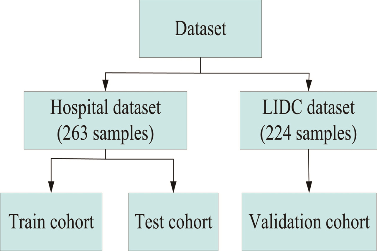
Two datasets allocation pattern diagram.

2.2 Image segmentation

We used 3Dslicer (Version 4.6.2; Surgical Planning Laboratory, Brigham and Women’s Hospital, MA, USA; http://www.slicer.org) to segment pulmonary nodules on CT images in Hospital Dataset. Three experienced thoracic radiology experts independently examined the CT images of a patient, and carefully analyzed the pictures of each layer, to confirm the edge of the pulmonary nodules.

In the LIDC dataset, pulmonary nodules were already segmented, which were defined by four radiologists independently. The edge-delimited data were stored in an XML file. We programmed a MATLAB program to read XML files and process DICOM data. All ROIs were extracted using Matlab R2017b.

The final segmentation results were determined by intersection Volume of interest (VOI) for each pulmonary nodule drawn by all the radiologists for both datasets. Figure 2 shows the segmentation results of nodules. The top three row shows the LIDC datasets, others bottom row shows the Hospital datasets.

Fig. 2

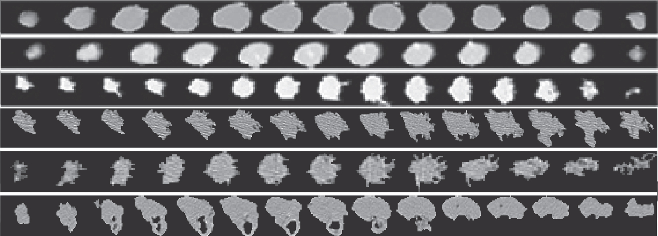
Segmentation results of two datasets.

2.3 Radiomic feature extraction

Each image area has its characteristics that can be differentiated from the different regions. Some features can be visually perceived, while others require mathematical transformation or processing. Radiomics can extract the visual and mathematical features utilized in the statistical model to solve the clinical problem.

We used a self-written Matlab script to extract 867 radiomics features in the VOI of lung nodules, including 14 one-dimensional imaging features, 12 basic shape and size features, 247 3D gray level co-occurrence matrix features, 44 2D grayscales run matrix (GLRL-2D) features, 11 3D gray area size matrix (GLSZM-3D) features, 496 Laws image texture features (Law-Textures), 27 LoG features including 2nd-order edge information, and 16 multi-scale 3D wavelet features.

2.4 Feature selection

This study used the FSLib_v6.2.1_2018 [32] toolbox to perform feature selection, a Matlab toolkit for data reduction and feature selection. In the toolbox, there are 19 kinds of methods. This toolbox contains 19 types of feature selection methods. We applied these selection methods to extract features of different scales (different number of the features, 50, 100, 200, 300, 400, 867) by the sorting way. In this paper, we showed the result of the top 10 methods by ranking the AUC (area under the receiver operator characteristic curve) to evaluate the predictive performance of different feature selection and classification methods. This feature selection procedure was carried out only using the Hospital Dataset.

2.5 Machine learning classification

To test the classification performance of the selected radiomics features, we trained 7 machine learning models for classification between benign and malignant pulmonary nodules using the Hospital Dataset: KNN, BAG, DT, NB, LDA, SVM, and RF (the abbreviation for each feature selection method and classification method was listed in Table 1). We divided data in the two datasets we mentioned before into three subsets, including training sets (237 training samples from the hospital), testing sets (26 test samples from the hospital), and validation sets (224 samples from LIDC).

Table 1
Abbreviations and full names of the ten feature selection methods and seven classification methods

abbreviations Feature selection method abbreviations Classification method

MRMR Minimum redundancy maximum relevance ensemble KNN k-nearest neighborhood

MI Mutual information BAG bagging

Relieff Relief-F DT Decision tree

Lasso Least absolute shrinkage and selection operator NB Naïve basyes

Fsv Feature selection via concave minimization LDA Linear discriminant analysis

L0 l0-norm regularization SVM Support vector machine

Fisher Fisher discrimination criterion RF Random forest

Mcfs Unsupervised feature selection for multi-cluster data

Cfs Correlation-based feature selection

Rfe Recursive feature elimination

abbreviations	Feature selection method	abbreviations	Classification method
MRMR	Minimum redundancy maximum relevance ensemble	KNN	k-nearest neighborhood
MI	Mutual information	BAG	bagging
Relieff	Relief-F	DT	Decision tree
Lasso	Least absolute shrinkage and selection operator	NB	Naïve basyes
Fsv	Feature selection via concave minimization	LDA	Linear discriminant analysis
L0	l0-norm regularization	SVM	Support vector machine
Fisher	Fisher discrimination criterion	RF	Random forest
Mcfs	Unsupervised feature selection for multi-cluster data
Cfs	Correlation-based feature selection
Rfe	Recursive feature elimination

2.6 Tuning parameters for machine learning models

In the current research area, parameter tuning is an essential element in classification studies. Kernel and mapping functions require parameter tuning and initialization in many studies [33]. Efficient parameter tuning is a crucial aspect of machine learning methods. But so far, there is no best way to choose the appropriate parameters. Grid Search is the most precise method for selecting the proper machine learning model.

However, grid search can be very computationally expensive and depends on data sampling. It is difficult to find the optimal parameter value with solid generalization ability. We used the most convenient variable control method to keep the parameters within a specific range in this experiment. We fixed most parameters and adjusted one to analyze the trend of this parameter. Thus, parameter tuning saved much time.

In this paper, we have two datasets. Patient samples from Hospital Dataset were randomly divided into a training cohort and a test cohort used to construct and test the proposed classifiers. The dataset from LIDC Dataset is served as the independent validation cohort. The predictive accuracy of the classifier was estimated using ROC curves and precision. For the robust stability of the machine learning algorithm, we did a permutation test that randomly repeated shuffled labels 1000 times.

3 Results

In this section, we describe the classification results obtained based on radiomics features for lung cancer diagnosis.

3.1 Feature selections

AUC assessed the predictive performance of different feature selection methods and classification methods. The top 10 feature selection methods for the highest AUCs were MRMR, MI, Relieff, Lasso, Fsv, L0, Fisher, Mcfs, Cfs, and Rfe (see Table 2). Our experimental results showed that some feature selection methods had a good performance. As the SVM obtained the highest AUC in feature selection, we took the SVM results of feature selection methods in different feature numbers.

Table 2
AUC results of 7 classified methods and 10 feature selection methods

NB KNN DT BAG LDA RF SVM

MRMR 0.672 0.6406 0.6308 0.6651 0.6009 0.7007 0.7057

MI 0.6411 0.6190 0.6509 0.7213 0.5854 0.7229 0.6787

Relieff 0.6225 0.6421 0.5527 0.6272 0.6013 0.6455 0.6293

Lasso 0.6488 0.6004 0.6256 0.6503 0.5873 0.6933 0.7004

Fsv 0.6752 0.6499 0.5915 0.6382 0.6922 0.6584 0.7646

L0 0.6707 0.6154 0.5932 0.6475 0.7047 0.6746 0.7405

Fisher 0.6440 0.6038 0.6423 0.7073 0.6073 0.7339 0.7160

Mcfs 0.6331 0.5323 0.6670 0.6576 0.5897 0.6690 0.6624

Cfs 0.6210 0.5760 0.6213 0.6641 0.5873 0.6556 0.6795

Rfe 0.5949 0.5537 0.6128 0.6799 0.6362 0.7035 0.6789

	NB	KNN	DT	BAG	LDA	RF	SVM
MRMR	0.672	0.6406	0.6308	0.6651	0.6009	0.7007	0.7057
MI	0.6411	0.6190	0.6509	0.7213	0.5854	0.7229	0.6787
Relieff	0.6225	0.6421	0.5527	0.6272	0.6013	0.6455	0.6293
Lasso	0.6488	0.6004	0.6256	0.6503	0.5873	0.6933	0.7004
Fsv	0.6752	0.6499	0.5915	0.6382	0.6922	0.6584	0.7646
L0	0.6707	0.6154	0.5932	0.6475	0.7047	0.6746	0.7405
Fisher	0.6440	0.6038	0.6423	0.7073	0.6073	0.7339	0.7160
Mcfs	0.6331	0.5323	0.6670	0.6576	0.5897	0.6690	0.6624
Cfs	0.6210	0.5760	0.6213	0.6641	0.5873	0.6556	0.6795
Rfe	0.5949	0.5537	0.6128	0.6799	0.6362	0.7035	0.6789

Figure 3 shows the trend chart of classification results of SVM extracted based on the different number of features. There is a fluctuating trend with the number of features and a high value near 100 parts. Curves were shown for the AUC trend chart with features increasing using different feature selection methods. The data of 100 elements are used for analysis in our later training.

Fig. 3

Trend of AUC with the increase of feature number.

Table 2 shows the results of the 100 features extracted from the 10 feature selection methods combined with 7 machine learning algorithms. The Fsv, L0, have good performance combined with SVM. The MI and Fisher have good classification accuracy combined with RF. Because RF and SVM have higher performance, we further performed parameter tuning for two machine learning algorithms. In this paper, we only showed the permutation test results of SVM.

The 20 selected features are given in Table 3, among which the first two columns are the features given by the 10 feature selection methods, the middle two columns are given by the Fsv method, and the last two columns are the features given by the L0 method. It can be seen that most of features given by the 10 methods are the statistical information under the original image, the Fsv method also gives more information about the first-order features under the original image, and the L0 method gives the statistical information after the LAW transformation.

Table 3

The feature selected by 10 methods, Fsv and L0

10method		Fsv		L0
5	mean	1	energy	398	L5W5W5.std
6	mean.absolute.deviation	2	entropy	399	L5W5W5.kur
1	energy	7	median	400	L5W5W5.ske
2	entropy	3	kurtosis	401	L5W5R5.ave
7	median	597	S5W5W5.ave	402	L5W5R5.std
8	mininum	5	mean	403	L5W5R5.kur
17	volume.cc	6	mean.absolute.deviation	404	L5W5R5.ske
4	maximum	13	uniformity	405	L5R5L5.ave
16	volume	16	volume	406	L5R5L5.std
9	range	66	contrast.03	407	L5R5L5.kur
15	surface.area	102	inverse.difference.04	409	L5R5E5.ave
13	uniformity	103	asm.05	392	L5W5E5.ske
14	variance	115	imc2.05	395	L5W5S5.kur
21	max.z.diameter	132	d.ent.06	396	L5W5S5.ske
29	correlation.01	437	E5L5W5.ave	397	L5W5W5.ave
40	autocorrelation.01	443	E5L5R5.kur	408	L5R5L5.ske
12	standard.divation	691	W5W5E5.kur	410	L5R5E5.std
22	surface.volume.ratio	853	LLL.sd	393	L5W5S5.ave
25	compactness1	35	ent.01	394	L5W5S5.std
3	kurtosis	54	ent.02	412	L5R5E5.ske

Figure 4 shows permutation test results of SVM classification. We trained the model 1000 times with a random disturb label and got a result p < 0.02.

Fig. 4

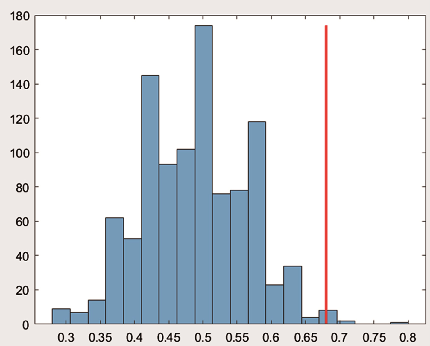
Permutation test results. The blue part is the distribution of the accuracy of 1000 random label results by SVM classification, and the red line is the accuracy provided by the original label.

3.2 Parameter tuning

We concluded that RF and SVM classifiers obtained better performance than other machine learning algorithms with default parameter settings. Therefore, we conducted parameter tuning only for these two methods.

3.2.1 Parameter tuning for SVM

We chose the ‘linear’ kernel function and adjusted the parameter c = [1–100]. We chose the ‘Poly’ kernel function and adjusted the parameter c = [1–250], degree = [1 –3], gamma = [0.01–0.3], coef0 = [0–100]. We chose the ‘Sigmoid’ kernel function and adjusted the parameter c = [1–150], gamma = [0.01–0.3], coef0 = [0–4]. We chose the ‘RBF’ kernel function and adjusted the parameter c = [1–150], gamma = [0.01–0.3].

(1) Linear kernel function

As shown from Fig. 5(a), when c values vary from 2 to 12, accuracy is above 0.74. c = 10 is the optimal value, at which point accuracy reaches its peak value at 0.77 and AUC = 0.837. When the kernel is Linear, c = 10, and other parameters are the default values, the ROC curve is shown in Fig. 5 (c) AUC = 0.837.

Fig. 5

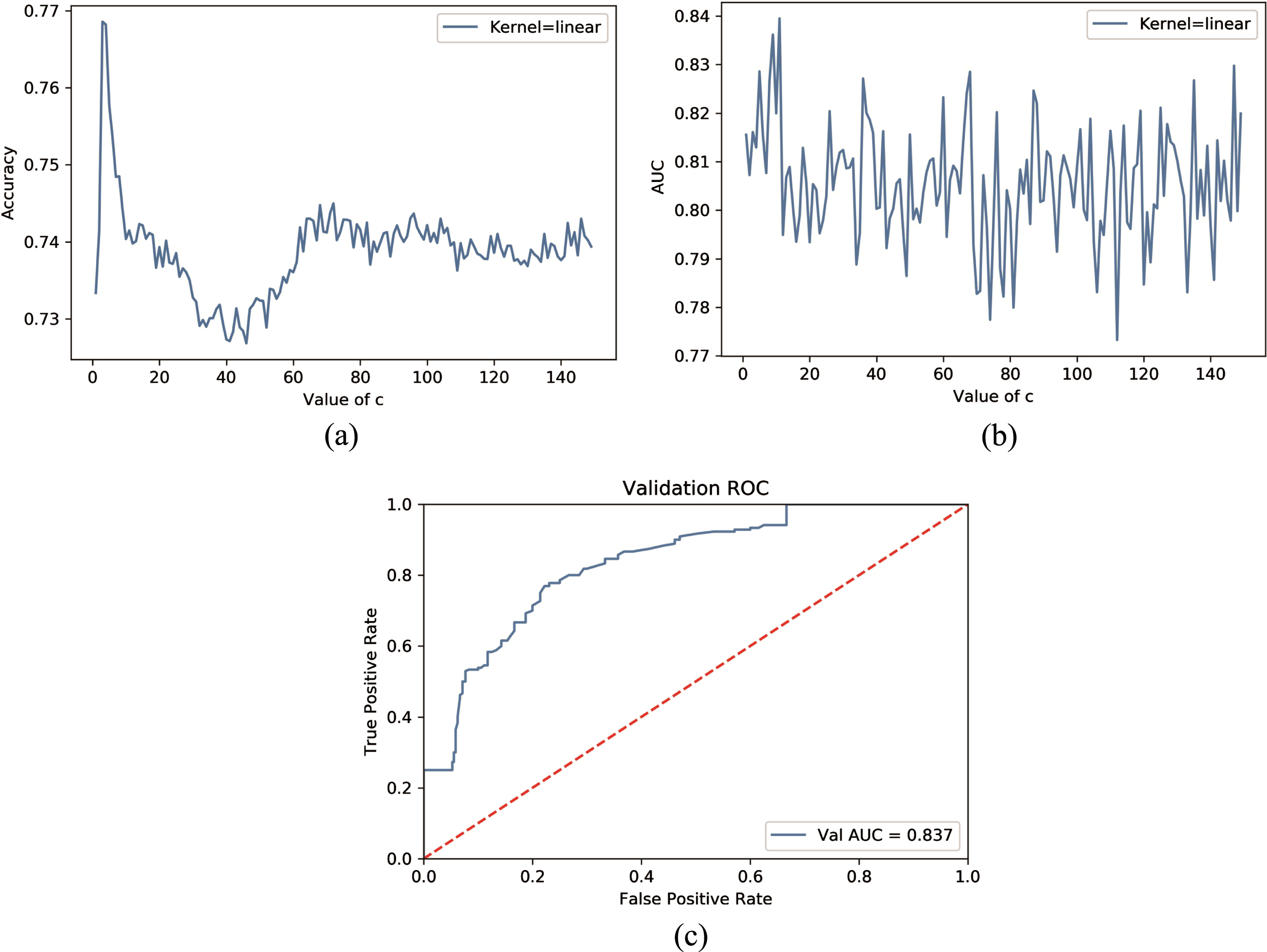
Linear kernel tuning of a SVM model with linear kernel. The diagrams show the response of model performance at different level of parameter c and the ROC curve of the model with best parameters. In (a) the horizontal axis in the figure indicates the value of parameter c, range from 0 to 140. different values of parameter c will have different effects on the accuracy of the model. In (b) AUC score of the model with different regularization parameter c. In (c) it shows the ROC curve of the SVM model with best parameter. Each point on the blue line represents false positive rate and true positive rate under different classification thresholds. The red dotted line denotes chance level.

(2) Poly kernel function

We see Fig. 6(a), we tune the c, other parameters are default values, the c value ranges from 125 to 225, and the accuracy is more significant than 0.76. c = 140 is the optimal value, and accuracy reaches its peak value at 0.768. We see the Fig. 6(b), when c = 140, degree = 1, coef0 = 0, and other parameters are default values, the gamma value ranges from 0.015 to 0.024, and the accuracy is above 0.75. Gamma = 0.028 is the optimal value, and accuracy reaches its peak value at 0.773. As for degree in Fig. 6(c), we see that less than 2 is better, so we set degree as 1. When the kernel is Poly, c = 140, degree = 1, coef0 = 0, gamma = 0.028 the ROC curve is shown in Fig. 6(d) AUC = 0.820.

Fig. 6

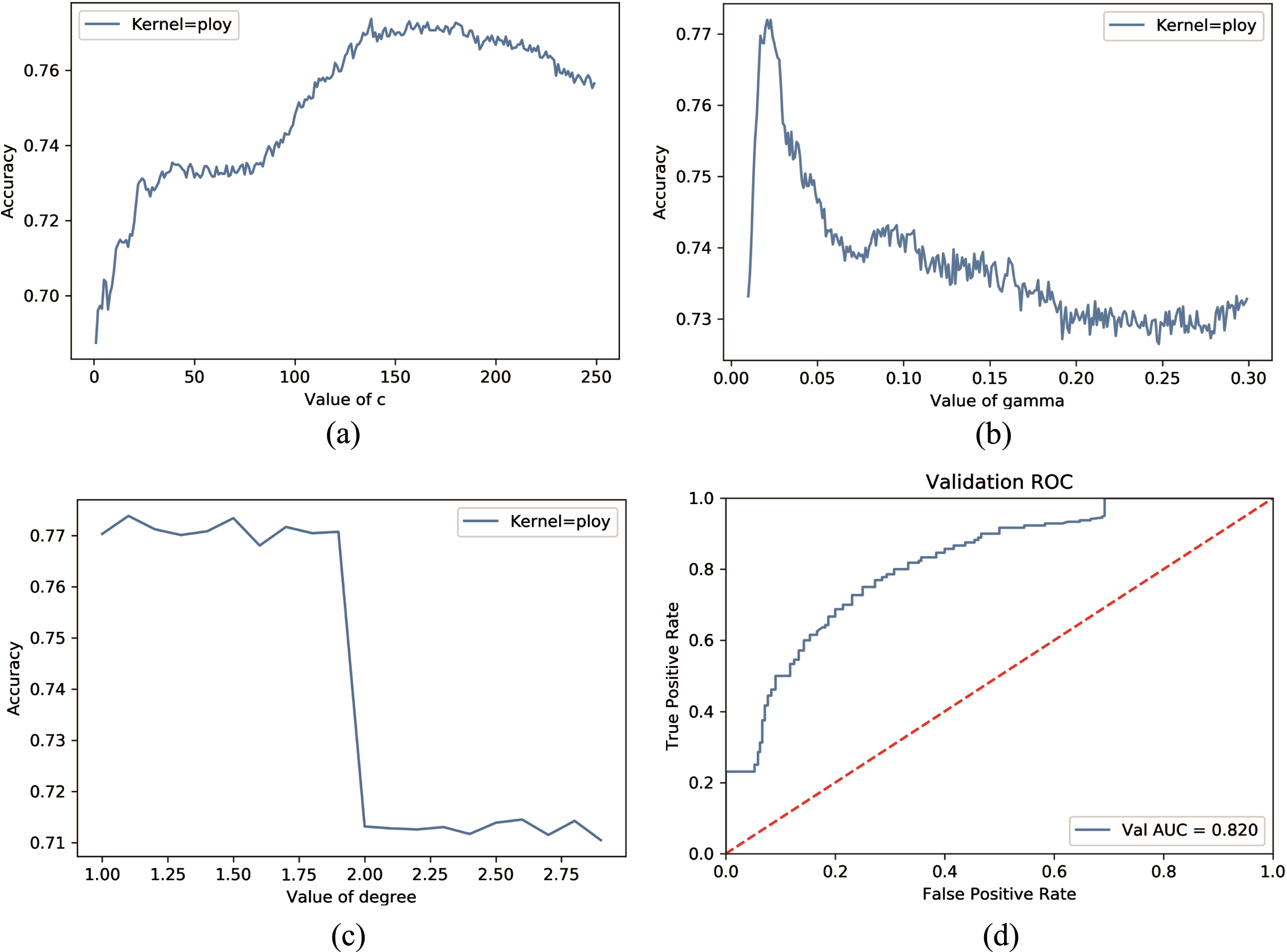
Poly kernel tuning of a SVM model with poly kernel, to choose the best parameters, we draw the curves of model accuracy score with different parameter at different level. (a) Accuracy score of the model with different regularization parameter c, when c = 140 the accuracy score of the model is the highest. (b) Fix the parameter c = 140, the curve shows the accuracy score of the model with different gamma values. In this context, gamma = 0.028 is the best. (c) Fix the parameter c = 140, gamma = 0.028, the curve shows the accuracy score of the model with different degree values. The accuracy score decreases sharply when change degree from 1 to 2. (d) Pictured the ROC curve of the model with the best value of c, gamma and degree.

(3) Sigmoid kernel function

According to the experimental results from Fig. 7(a), when the kernel is sigmoid, the optimal value of c is 28, and the optimal value and the accuracy are 0.727. As shown in Fig. 7(b), when c = 28, coef0 = 0, and other parameters are default values, gamma is between 0.003 and 0.027. Gamma = 0.016 was the optimal value, and accuracy reached a peak value at 0.735. We can see from Fig. 7(c) that coef = 0 is the best answer. When the kernel is sigmoid, c = 28, coef0 = 0, gamma = 0.016, and other parameters are default values; Fig. 7(d) show the ROC curve, AUC = 0.802.

Fig. 7

Sigmoid kernel tuning of a SVM model with sigmoid kernel, to choose the best parameters, we draw the curves of model accuracy score with different parameter at different level. (a) Accuracy score of the model with different regularization parameter c. when c = 28, the accuracy score of the model is the highest. (b) Fix the parameter c = 28, the curve shows the accuracy score of the model with different gamma values. In this context, gamma = 0.016 is the best. (c) Fix the parameter c = 28, gamma = 0.016. The accuracy score is highest at coef = 0. (d) Pictured the ROC curve of the model with the best value of c, gamma and coef.

(4) RBF kernel function

According to the experiment, when the kernel is RBF, the optimal value of C is 35. As shown in Fig. 8(a), when C = 35 and other parameters are default values, the accuracy is above 0.74. Gamma =0.021 is the optimal value, and accuracy reached its peak value at 0.733. When the kernel is RBF, C = 35, gamma = 0.021, and other parameters are default values, the ROC curve is shown in Fig. 8(c) AUC = 0.805.

Fig. 8

RBF kernel tuning of a SVM model with RBF kernel, to choose the best parameters, we draw the curves of model accuracy score with parameter c and gamma at different level. (a) Value of c ranges from 0 to 140, the accuracy score of model classification reaches its highest at c = 35. (b) Fix the parameter c = 35, the curve shows the accuracy score of the model with different gamma values. In this context, gamma = 0.021 is the best. (c) Pictured the ROC curve of the model with the best value of c and gamma.

3.2.2 Tuning random forest model’s parameters

We select the n_estimators = [10–1000]; min_samples_split = [0.01–1]. The results are shown in Fig. 9.

Fig. 9

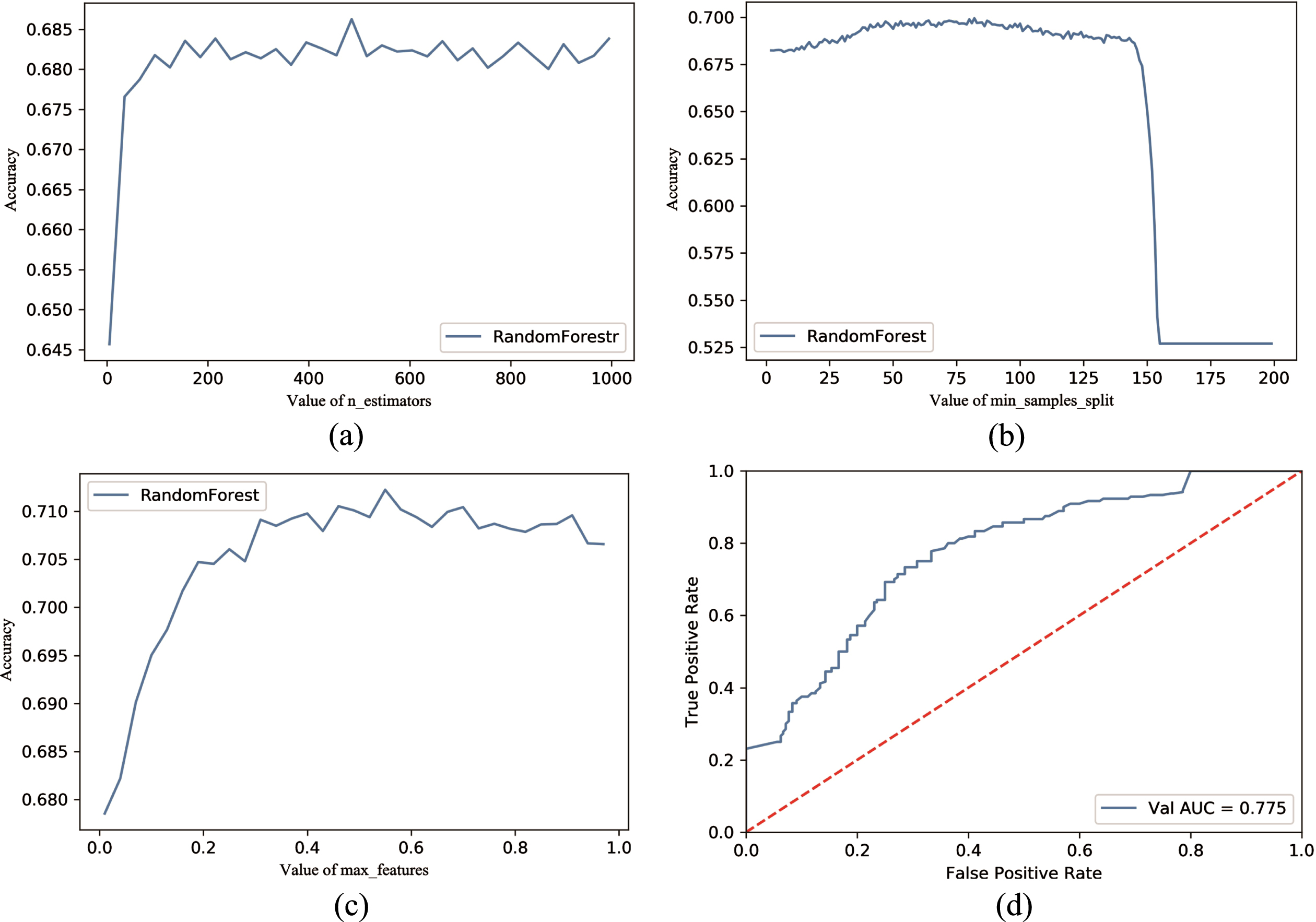
Random Forest tuning. As for random forest model, we plotted the curves to show the effect of different values of different parameters on the accuracy of the model. (a) The accuracy score of model with different number of base estimators. number of base model saturated when the n_estimators value is above 150. (b) The accuracy score of the model with different value of the minimum number of samples required to split an internal node. (c) The accuracy score of the model with different value of the number of features to consider when searching for the best split. (d) ROC curve of the model with the best value of n_estimators, min_samples_split, and max_feature.

Figure 9(a) indicates the range of AUC when the value of n_estimators is from 0 to 1000. Here we first choose min_samples_split = 2, max_features=’auto’, and other parameters are default values. When the n_estimators value is above 150, the accurate value tends to be stable and has small fluctuation. when the value range of n_estimators is between 490 and 530, the accuracy is above 0.68, n_estimators = 510 is the optimal value. Figure 9(b) shows the value accuracy of min_sapmlse_split; while min_samples_split is less than 150, the results are stable. Accuracy clearly shows a downward trend and suddenly drops when the value is 155. Figure 9(c) shows the accuracy range when the value of max_features is from 0 to 1. When the max_feature value is above 0.5, the accurate value tends to be stable and has small fluctuation. When the n_estimators = 510, min_samples_split = 8, and max_feature = 0.55, the ROC curve is shown in Fig. 9(d) AUC = 0.775.

3.3 Cross-dataset validation

Based on the finding in 3.2, we obtained an appropriate machine learning model by tuning parameters for data in the hospital dataset. We then used data in the LIDC dataset for verification. If using SVM as classifier, and the kernel is Poly, C = 140, degree = 1, coef0 = 0, gamma = 0.028, we obtained AUC = 0.78. While utilizing RF classifier, and max_features = 0.55, min_samples_split = 8, n_estimators = 510, we obtained AUC = 0.77.

In generally, we found that the parameters-adjusted model had obtained preferable results for data verification in multi-center. We can increase the predictive performance of the model through tuning parameters in a dataset (single-center). But different machine learning models exhibit different generalization capabilities.

The ROC curves of the SVM model and the RF model in the training set, test set and validation set are given in Fig. 10 (a) and Fig. 10 (b), respectively, and it can be seen that both models can be implemented for radiomics studies.

Fig. 10

(a) ROC curves in training set (yellow line), validation set (green line) and test set (blue line) of SVM model with best parameters. (b) ROC curves in training set (yellow line), validation set (green line) and test set (blue line) of RF model with best parameters.

4 Discussion

Lung cancer is one of the high mortality cancers in the world [33]. Early diagnosis plays an essential role in it. Radiomics can extract and analyze image data through high-throughput texture features, improving doctors’ diagnostic efficiency and accuracy. Radiomics converts medical imaging into mineable data through the high-throughput extraction of quantitative measures from regions of interest. These high-dimensional radiomics feature sets can be distilled into diagnoses and predictions paired with machine learning algorithms. Based on the research of lung cancer diagnosis data of radiomics, this paper analyzes and studies different feature selection methods and machine learning methods. The research found that the diagnosis accuracy can be improved by adjusting the parameters of machine learning and feature selection.

Notably, a parameter tuning of machine learning had a more outstanding performance and robustness than no tuning for the radiomics study. The analysis results have the potential to guide treatment strategies better.

When the number of extracted features in radiomics research reported in some pieces of literature is small (less than 50), a higher AUC can be obtained [34 –37]. However, in this paper, the number of extracted features is much larger than that reported above, indicating that the number of extracted radiomics features in different data sets and which type of radiomics provide a higher basis are uncertain.

Feature selection methods are also used for different data sets [38]. Modeling and testing have low AUC values across data sets. There are significant differences in the data set. When we extracted features, we found that the features extracted by each algorithm were different. If we want to see the parts that contribute the most to classification, we can’t remove them by combining several feature extraction methods. In this paper, the best performance of SVM based model in the feature selection method is Fsv and l0. The best version of the RF-based model is Mi and Fisher algorithm.

We study the parameter adjustment of machine learning according to the extracted features and find that the AUC value can be improved by adjusting the parameters of machine learning; that is, the results obtained by using the default parameters can be improved by changing the parameters, which can be improved by about 5% –10% in general.

We investigated a machine learning model with parameter tuning in a multi-center dataset. We found that quantitative radiomic features extracted from CT of the lung nodules could successfully differentiate between malignant and benign tumors. Parameter tuning can improve the performance of machine learning methods. Using independent testing datasets is an accurate method to verify the model’s generalization performance. By cross-validated analysis, the radiomics model achieved good predictive performance with an average AUC at 0.75 for the differentiation of malignant and benign lung nodules. The selection of the machine learning model and the adjustment of parameters can significantly improve the effectiveness of the machine learning model. With tuning parameters of the model, a more precise model is built, and more accurate data analysis results can be obtained.

There are also several limitations in our study. First, the dataset in this study is medium size. The more patient samples we analyze, the more stable model we could obtain. Second, the current study only focused on diagnosing benign and malignant lung cancer but not on estimating the level of malignancy. We plan to collect more pathological results for further verification in a multi-center dataset. Finally, we did not concretely analyze the specific meaning of the radiomics features we chose. We plan to do further analysis of the relationship between radiomics signatures and clinicopathological features. Nevertheless, getting the clinical significance of these features is quite essential, and further study is needed.

Footnotes

Acknowledgments

This work was supported by the Tianjin natural science foundation (18JCYBJC95600) and the National Scientific Foundation of China (81974277, 81000639).

Conflict of interest

There are no relationships with companies whose products or services may be related to the article’s subject matter.

References

Wilson

and Devaraj

, Radiomics of pulmonary nodules and lung cancer, Translational Lung Cancer Research 6(1) (2017), 86.

Bae

J.M.

, Jeong

J.Y.

, Lee

H.Y.

, et al., Pathologic stratification of operable lung adenocarcinoma using radiomics features extracted from dual energy CT images, Oncotarget 8(1) (2017), 523.

Gillies

R.J.

, Kinahan

P.E.

and Hricak

, Radiomics: Images are more than pictures, they are data, Radiology 278(2) (2016), 563–577.

Napel

, Mu

, Jardim-Perassi

B.V.

, et al., Quantitative imaging of cancer in the postgenomic era: Radio (Geno) mics, deep learning, and habitats, Cancer 124(24) (2018), 4633–4649.

Bodalal

, Trebeschi

, Nguyen-Kim

T.D.L.

, et al., Radiogenomics: bridging imaging and genomics, Abdominal Radiology 44(6) (2019), 1960–1984.

Tunali

, Gray

J.E.

, Qi

, et al., Novel clinical and radiomic predictors of rapid disease progression phenotypes among lung cancer patients treated with immunotherapy: An early report, Lung Cancer 129 (2019), 75–79.

Trebeschi

, Drago

S.G.

, Birkbak

N.J.

, et al., Predicting response to cancer immunotherapy using noninvasive radiomic biomarkers, Annals of Oncology 30(6) (2019), 998–1004.

Feng

, Chen

, et al., Differentiating minimally invasive and invasive adenocarcinomas in patients with solitary sub-solid pulmonary nodules with a radiomics nomogram, Clinical Radiology 74(7) (2019), 570–e1.

She

, Zhang

, Zhu

, et al., The predictive value of CT-based radiomics in differentiating indolent from invasive lung adenocarcinoma in patients with pulmonary nodules, European Radiology 28(12) (2018), 5121–5128.

10.

Mei

, Luo

, Wang

and Gong

, CT texture analysis of lung adenocarcinoma: can radiomic features be surrogate biomarkers for EGFR mutation statuses, Cancer Imaging 18(1) (2018), 52.

11.

Jia

T.Y.

, Xiong

J.F.

, Li

X.Y.

, et al., Identifying EGFR mutations in lung adenocarcinoma by noninvasive imaging using radiomics features and random forest modeling, European Radiology 29(9) (2019), 4742–4750.

12.

Wang

, Zhao

, Li

, et al., Can peritumoral radiomics increase the efficiency of the prediction for lymph node metastasis in clinical stage T1 lung adenocarcinoma on CT, European Radiology 29 (2019), 6049–6058.

13.

Moran

, Daly

M.E.

, Yip

S.S.F.

, et al., Radiomics-based assessment of radiation-induced lung injury after stereotactic body radiotherapy, Clinical Lung Cancer 18(6) (2017), e425–e431.

14.

, Mu

, Balagurunathan

, et al., Multi-window CT based radiomic signatures in differentiating indolent versus aggressive lung cancers in the National Lung Screening Trial: a retrospective study, Cancer Imaging 19(1) (2019), 45.

15.

Digumarthy

S.R.

, Padole

A.M.

, Rastogi

, et al., Predicting malignant potential of subsolid nodules: can radiomics preempt longitudinal follow up CT? Cancer Imaging 19(1) (2019), 36.

16.

, Tao

, Zhu

, et al., Prediction of pathologic stage in non-small cell lung cancer using machine learning algorithm based on CT image feature analysis, BMC Cancer 19(1) (2019), 464.

17.

Zhang

, Yuan

, Zhong

, et al., Differentiation of focal organising pneumonia and peripheral adenocarcinoma in solid lung lesions using thin-section CT-based radiomics, Clinical Radiology 74(1) (2019), 78.E23–78.E30.

18.

Sun

, Hu

, Ge

, et al., Radiomics study for predicting the expression of PD-L1 in non-small cell lung cancer based on CT images and clinicopathologic features, Journal of X-ray Science and Technology 28(3) (2020), 449–459.

19.

Haga

, Takahashi

, Aoki

, et al., Standardization of imaging features for radiomics analysis, The Journal of Medical Investigation 66(1.2) (2019), 35–37.

20.

Peeken

J.C.

, Bernhofer

, Spraker

M.B.

, et al., CT-based radiomic features predict tumor grading and have prognostic value in patients with soft tissue sarcomas treated with neoadjuvant radiation therapy, Radiotherapy and Oncology 135 (2019), 187–196.

21.

Luo

, Xu

, Zhang

, et al., Radiomic features from computed tomography to differentiate invasive pulmonary adenocarcinomas from non-invasive pulmonary adenocarcinomas appearing as part-solid ground-glass nodules, Chinese Journal of Cancer Research 31(2) (2019), 329.

22.

Leger

, Zwanenburg

, Pilz

, et al., CT imaging during treatment improves machine learning models for patients with locally advanced head and neck cancer, Radiotherapy and Oncology 130 (2019), 10–17.

23.

Theek

, Opacic

, Magnuska

, et al., Radiomic analysis of contrast-enhanced ultrasound data, Scientific Reports 8(1) (2018), 11359.

24.

Tunali

, Gray

J.E.

, Qi

, et al., Novel clinical and radiomic predictors of rapid disease progression phenotypes among lung cancer patients treated with immunotherapy: An early report, Lung Cancer 129 (2019), 75–79.

25.

Vandendorpe

, Durot

, Lebellec

, et al., Prognostic value of the texture analysis parameters of the initial computed tomographic scan for response to neoadjuvant chemoradiation therapy in patients with locally advanced rectal cancer, Radiotherapy and Oncology 135 (2019), 153–160.

26.

Yin

, Yang

, Tang

, et al., Enhanced computed tomography radiomics-based machine learning methods for predicting the Fuhrman grades of renal clear cell carcinoma, Journal of X-ray Science and Technology 29(6) (2021), 1149–1160.

27.

Lee

S.H.

, Cho

H.H.

, Lee

H.Y.

and Park

, Clinical impact of variability on CT radiomics and suggestions for suitable feature selection: a focus on lung cancer, Cancer Imaging 19(1) (2019), 54.

28.

Sun

, Wang

, Mok

V.C.

and Shi

, Comparison of Feature Selection Methods and Machine Learning Classifiers for Radiomics Analysis in Glioma Grading, IEEE Access 7 (2019), 102010–102020.

29.

Clark

, Vendt

, Smith

, et.al., The Cancer Imaging Archive (TCIA): Maintaining and Operating a Public Information Repository, Journal of Digital Imaging 26(6) (2013), 1045–1057.

30.

Armato

S.G.

3rd, McLennan

, Bidaut

, et al., The Lung Image Database Consortium (LIDC) and Image Database Resource Initiative (IDRI): A completed reference database of lung nodules on CT scans, Medical Physics 38(2) (2011), 915–931.

31.

LIDC-IDRI, https://wiki.cancerimagingarchive.net/display/Public/LIDC-IDRI.

32.

Feature Selection Library (https://www.mathworks.com/matlabcentral/fileexchange/7-feature-selection-library), MATLAB Central File Exchange. Retrieved February 18, 2021.

33.

Binczyk

, Prazuch

, Bozek

and Polanska

, Radiomics and artificial intelligence in lung cancer screening, Translational Lung Cancer Research 10 (2021), 1186–1199.

34.

Chang

, Sun

X.Y.

, Wang

, et al., A Machine learning model based on PET/CT radiomics and clinical characteristics predicts ALK rearrangement status in lung adenocarcinoma, Frontiers in Oncology 11 (2021), 603882.

35.

B.X.

, Song

Y.X.

, Wang

L.L.

, et al., A machine learning-based prediction of the micropapillary/solid growth pattern in invasive lung adenocarcinoma with radiomics, Translational Lung Cancer Research 10(2) (2021), 955–964.

36.

Xie

Y.M.

, Zhao

H.G.

, Guo

, et al., A PET/CT nomogram incorporating SUVmax and CT radiomics for preoperative nodal staging in non-small cell lung cancer, European Radiology 31 (2021), 6030–6038.

37.

Zhang

, Jin

J.B.

, Ai

, et al., Computer tomography radiomics-based nomogram in the survival prediction for brain metastases from non-small cell lung cancer underwent whole brain radiotherapy, Frontiers in Oncology 10 (2021), 610691.

38.

Yang

, Chen

, Wei

H.F.

, et al., Machine learning for histologic subtype classification of non-small cell lung cancer: A retrospective multicenter radiomics study, Frontiers in Oncology 10 (2021), 608598.