Cardiac CT motion artifact grading via semi-automatic labeling and vessel tracking using synthetic image-augmented training data

Abstract

Cardiac CT provides critical information for the evaluation of cardiovascular diseases. However, involuntary patient motion and physiological movement of the organs during CT scanning cause motion blur in the reconstructed CT images, degrading both cardiac CT image quality and its diagnostic value. In this paper, we propose and demonstrate an effective and efficient method for CT coronary angiography image quality grading via semi-automatic labeling and vessel tracking. These algorithms produce scores that accord with those of expert readers to within 0.85 points on a 5-point scale. We also train a neural network model to perform fully-automatic motion artifact grading. We demonstrate, using XCAT simulation tools to generate realistic phantom CT data, that supplementing clinical data with synthetic data improves the scoring performance of this network. With respect to ground truth scores assigned by expert operators, the mean square error of grading motion of the right coronary artery is reduced by 36% by synthetic data supplementation. This demonstrates that augmentation of clinical training data with realistically synthesized images can potentially reduce the number of clinical studies needed to train the network.

Keywords

Cardiac CT motion artifacts semi-automatic labeling vessel tracking deep learning

1 Introduction

Cardiovascular disease (CVD) is the global leading cause of death [1]. Among CVDs, atherosclerosis of the coronary arteries is the principal cause of morbidity and mortality [2]. Many different cardiac imaging techniques enable to assess the presence and progression of coronary artery diseases (CADs), in which intrusive plaques form in the arterial wall. Coronary computed tomography angiography (CTA) is an advanced x-ray imaging technique which provides 4-dimensional (4D) high resolution volumetric images of the moving heart and associated vessels. It has been reported that coronary CTA is the most accurate approach for diagnosis of CADs [3]. The use of CTA as the standard care for CVD patients has the potential to decrease the five-year rate of death from CAD [4]. However, there are some constraints on its applications. The quality of a CT image depends directly on the radiation dose, and high radiation exposure can cause harmful effects to patients [5]. Earlier work optimizes the radiation dose for CT by adjusting scanning parameters [6]. The higher the imaging radiation dose level, the lower the image noise level, and the better low-contrast structures may be visualized. It is not straightforward to obtain acceptable image quality for accurate clinical diagnosis at lower radiation dose levels [7].

Cardiac CT is particularly challenging because of the small size of vessels, rapid vessel motion, and the involuntary movement of patients. Cardiac CT requires a high resolution in order to resolve arterial stenoses, and requires image obtained at different phases of the cardiac cycle for dynamic imaging. To address these requirements, algorithms that yield high image quality at low doses are being developed [8, 9]. In cardiac CT, motion-induced blurring is unavoidable because motion leads to inconsistency between the acquired projections. Blurring makes it difficult to clearly visualize the vessels and accurately diagnose CAD. Many researchers are working to develop effective algorithms for motion correction [10 –12].

To evaluate the image quality of vessels, a primary step is to correctly determine vessel position. Here, we will develop a deep learning-based approach. Although deep learning (DL) methods were developed in the general computer vision field, they have been widely extended to image classification, image segmentation, image denoising, and super-resolution for specialized fields such as medical imaging. DL has demonstrated the ability to perform clinical decision making that is on a par or exceeds that of expert human operators [13 –19]. However, large and well-labelled datasets are required to train a good neural network model, and it is very challenging in cardiac CT to collect sufficient expert-labeled data. First, to collect real data from a patient, the patient needs a clinical indication for scanning, consent to the use of data for study, and to incur radiation dose. Second, expert skills are needed to label the data, and it is very time-consuming for radiologists to label each slice at every phase for every patient. Third, although data augmentation can help to overcome the overfitting issue that is commonly encountered in DL (e.g., using a convolution neural network and generative adversarial network to augment the data), a robust network that is pre-trained using a large real dataset is required to ensure that the network is not susceptible to any hidden bias [14, 17].

Traditional data augmentation methods (e.g., rotation, scaling) are not sufficient for cardiac CT given its 4D nature. To reduce the difficulty of collecting real data and providing accurate labels, an alternative approach is to generate realistic simulated images with many different anatomical variations in order to enlarge the size of training dataset. Synthetic and simulation data are currently used in medical image processing to enlarge datasets [20]. The projections generated by software can simulate realistic patent motion and reproduce motion blurring in cardiac CT images. Learning from simulated 4D images has the potential to enhance neural network model performance when applied to real images for a given task. However, it is essential to evaluate the generated data to ensure that datasets contain all the features needed to train a network, while being perceptually similar to real data. For simulated data, the analysis and evaluation are also very important processes. Objective methods for assessing human-perceived image quality attempt to quantify the visible errors between distorted and reference images using known properties of human vision system [21]. Objective image quality metrics can be used to classify the motion artifacts. In this work, structural similarity (SSIM) is employed to evaluate the image quality relative to the distortion-free image. The closer the SSIM value is to 1.0, the better the image quality is, and the less pronounced the motion artifacts.

In this paper, we present three contributions to semi-automatic labeling on simulated data. First, we utilize XCAT simulation tools to generate realistic data, leading to a fairly large dataset. Second, we introduce an auto-labeling method that is intended to reduce manual labelling effort. Third, we show that neural network classification performance on real data can be improved by adding labeled synthetic data to the training set.

2 Materials and methods

In this work, we generate realistic simulated data, which we use as training data, as well as to augment clinical training data. We also develop an automatic cardiac CT motion artifact grading method, which we then apply to clinical datasets. First, the datasets of both real and synthetic data are obtained, as well the corresponding labels for three major coronary arteries. GE Healthcare provided 4D CT images of 10 patients, and 20 image slices were selected for each patient. The real data images were graded for coronary motion artifacts by a well-trained expert operator, and this labeling was confirmed by radiologists at GE Healthcare and served as ground-truth scores for network training. The simulated data are labeled by the developed semi-automatic labeling method. Second, motion artifacts classification results are evaluated using the same model. A commonly used neural network with proven performance in this domain is chosen as the backbone network. The model is trained in three ways: a) by using real data only, b) using combined real and simulated data, and c) using simulated data only. Our objective is to determine whether a model trained on combined data can exceed the performance of one trained using real data only. In this paper, the task is to score the CT image quality on three major vessels in terms of motion artifacts. Task performance is rated as the accuracy of the scoring results with respect to the ground truth labels, and it is quantified by the average difference between the reference and the predicted scores. Two loss functions are used to evaluate the performance, L₁ loss and MSE loss.

To label the simulated data, we first generate the most representative reconstruction images by setting appropriate parameters in the simulation software. Then, for each generated data sample, we focus on the three major vessels (right circumflex artery [RCX], right coronary artery [RCA], and left anterior descending artery [LAD]) that are the most important vessels for the diagnosis of CAD. We track these vessels throughout the cardiac cycle in adjacent cardiac phases within the same slice to locate their positions. Finally, we use linear and non-linear models to label the corresponding vessels in terms of motion artifact grade and evaluate the labeling results.

2.1 Data simulation process

We use the 4D extended cardiac-torso (XCAT) phantom version 2 to generate cardiac CT phantoms. This widely used multimodality phantom was developed at Duke University and is described in detail in [22]. To simulate realistic dynamic cardiac CT images, XCAT outputs a 4D attenuation coefficient phantom to mimic a patient with beating heart. Phantoms are generated for a set of pre-defined parameters, including spatial resolution, temporal resolution, respiration rate, and heart rate. After generating the digital phantoms, we use XCAT’s CT projector software to simulate the cone-beam CT projection process. The CT projection simulation is controlled by some key parameters, such as the distance from the object to the source, the distance from the object to the detector, the detector array size, the x-ray source energy spectrum, and the beam half-fan angle. These key parameters are configured to simulate a representative GE CT scanner. Notably, to ensure the simulated CT images have similar noise level to real cardiac CT, we carefully tune the milliampere-seconds (mAs) parameter. In this study, mAs is set to 0.25 to match real data. After generating the projection data using circular scan, the standard FDK algorithm is employed to reconstruct the 3D volumetric image for each phase and scaled into Hounsfield Unit (HU) value image. Based on the tuned parameters, simulated images are generated for 10 males and 10 females. We reconstruct images at phases from 20% to 80% with an interval of 3%. For each simulated human phantom, this yields 21 different motion-blurred phases. In Figs. 1 2, the red circles in the motion-blurred and motion-free images show that the simulated images realize a motion blurring effect that is similar to that apparent in real cases. It is important to note that the synthetic data and the traditional augmentation data are based on different instances of “patient” anatomy, i.e., the synthetic data are not based on the existing training data, but purely on different realizations of the XCAT phantom.

Fig. 1

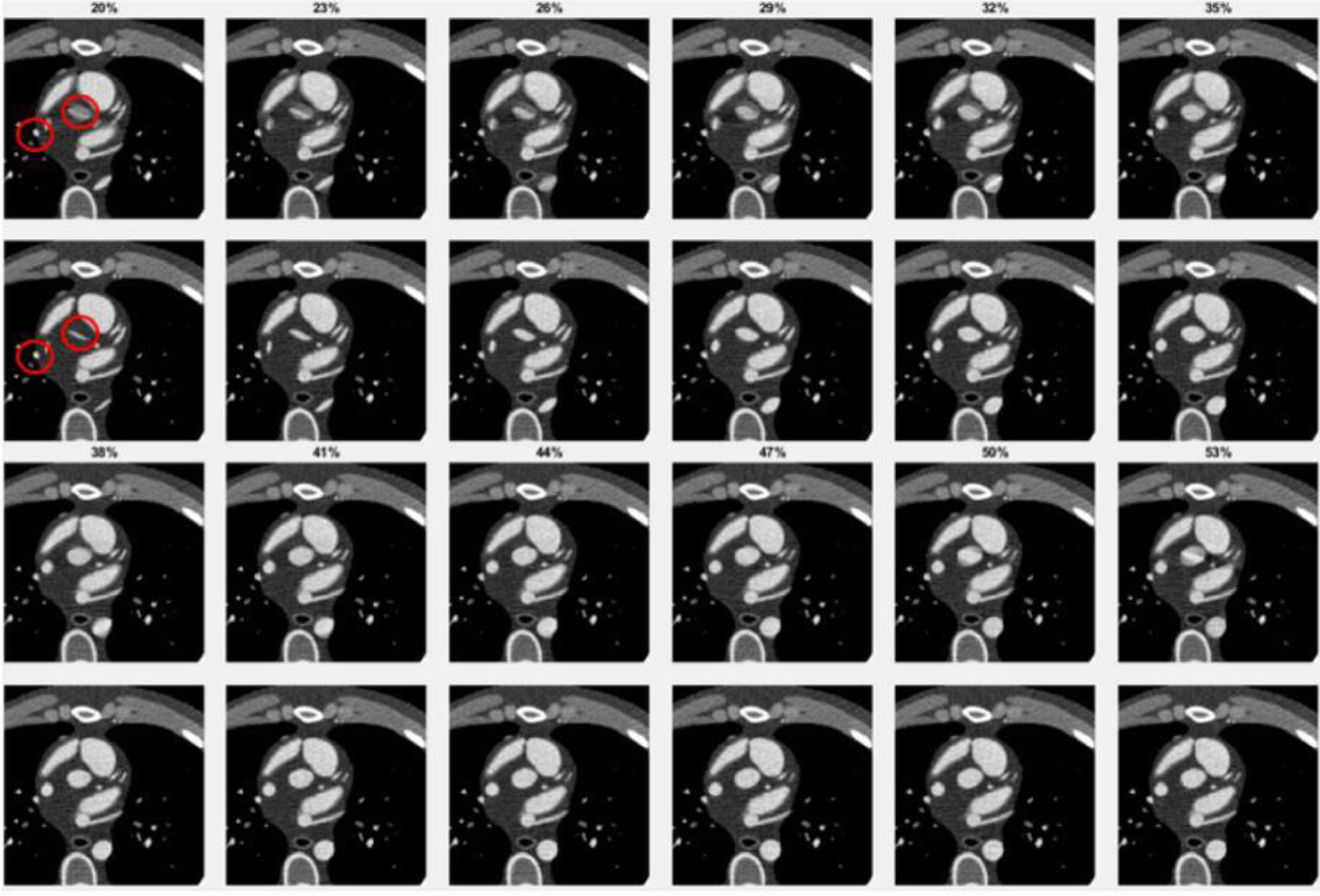
Simulated motion-blurred images (first and third rows) and the corresponding ground-truths (second and fourth rows) for 12 phases of a representative slice.

Fig. 2

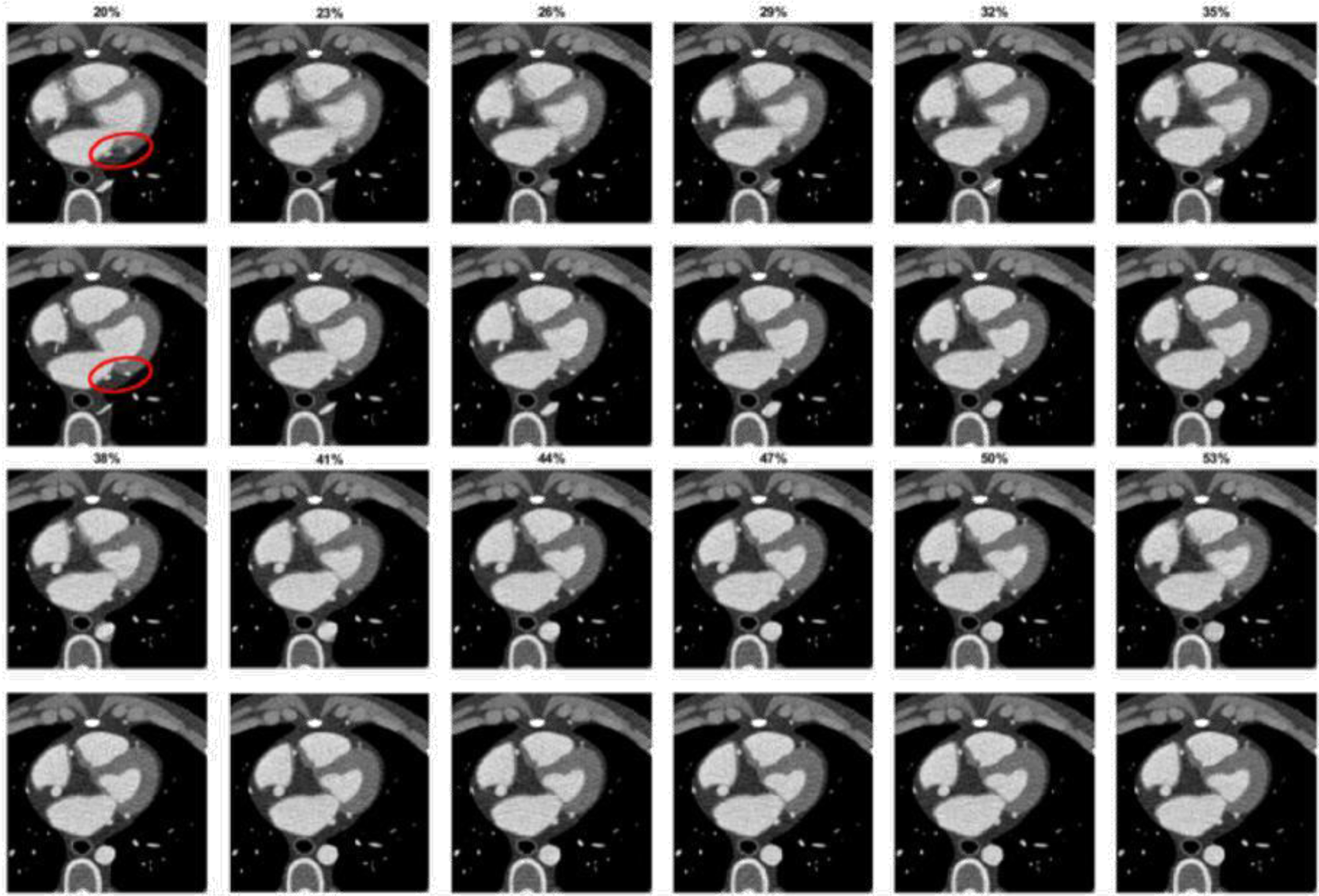
Simulated motion-blurred images, as described in Fig. 1, except showing a different image slice.

2.2 Data analysis and evaluation methods

In this paper, we use the structural similarity (SSIM) index as metric to track the major vessels and score the corresponding image quality for motion artifacts. The SSIM value represents the similarity between the reference and the distorted images. The value range of SSIM is from 0 to 1.0. The closer to 1.0 the SSIM value is, the better the image quality is with respect to the reference. For vessel tracking, the image patch in the previous slice/phase serves as the reference. For motion artifact evaluation, the motion-free image patch or the best one identified by an expert reader serves as the reference. To measure the performance of the motion artifacts evaluation model, we compute the mean square error between the model output and the ground truth. For real images, the ground truths are expert-assigned labels. For synthetic 4D images, ground truths are labeled by a semi-auto scoring method by comparing with the artifact-free phantom images, as we now describe.

2.3 Sliding window and vessel tracking

We are interested in evaluating three major vessels affected by CAD. Hence, we focus on small image patches covering these major vessels instead of the whole volumetric image. This narrows down the region of interest. However, due to patient and organ motion during the scanning process, vessel locations change between phases. Since the vessel displacement between two adjacent phases is small, once the location of a vessel in one phase is determined, its location in adjacent phases can be tracked by computing a similarity metric within the same patch size using a sliding window. The new position in the adjacent phase can be estimated by finding the maximum SSIM value in a search window.

In the preparation step, a sliding window is used to find each best patch in different phases within each slice. To achieve this, a reference phase image must be chosen. In this method, the reference image is the image which an expert operator selects as that phase least affected by motion artifacts. At the same time, the corresponding patch sizes are also chosen. The reconstructed image size is 256×256, covering an area of 192×192 mm², and we choose window sizes of 20, 26 and 32.

In the reference image, we position the window so that the vessel is at its center. To avoid potential error, the sliding window searches only a few pixels around the reference. The location with the best SSIM with respect to the reference is selected. This process involves searching only the immediately adjacent phases/slices. Once a match is found, this position becomes the new reference for the next phase/slice. This process is repeated for all phases/slices. In the final step, the initial reference image is employed to evaluate the quality of other phase/slice images in order to obtain quantitative SSIM values. A sequence of SSIM values will thus be obtained by comparing all phases to the reference phase.

2.4 Linear and non-linear scoring with mask

For each slice of the 4D volumetric image that contains 21 phases and corresponding SSIM values, we use a linear model to map the SSIM values to 5 categories (1 to 5) using a linear mapping. Category 1 represents patches with the most motion artifact, while category 5 patches have the least blurring. In the linear model, the same increment or decrement of SSIM value will cause the score increase or decrease by the same amount. Parameters of this linear model can be tuned to make the classification results closer to the real labels. Since the SSIM and motion score may not be linearly related, a non-linear model (e.g., k-means or support vector machine) can classify the SSIM values. However, the non-linear model is more dependent on data properties. For example, with the k-means method, the classification result may change when more data are added to the input data.

After patch locations are determined for all the phases and slices, each image patch includes not only the target vessel, but also the surrounding tissues. We adopt a mask methodology to focus on the vessel cross sections and thus reduce interference due to background pixels. To form the mask, we find a polygon that contains the vessel in all phases. Since the utility of including surrounding tissue is unknown, we evaluate performance with and without application of the mask.

2.5 Deep learning method

To demonstrate the effectiveness of the proposed method, some comparison tests are performed using a simple backbone network where we append two multilayer perceptrons (MLPs) (with 100 neurons for feature extraction, followed by one neuron for regression or six for classification to the output of ResNet-18) [23]. We choose to use a residual network (ResNet) because its skip connections address the network degradation problem otherwise encountered with deep neural networks containing many layers. The commonly used ResNet structures include ResNet-18, ResNet-34, ResNet-50, ResNet-101 and ResNet-152, where the numbers indicate the numbers of the layers. Given our dataset size and the problem complexity, ResNet18 is a best fit for our application. This network is first pretrained on the ImageNet-11k dataset, and then trained and tested on our dataset. We employ the following settings: batch size = 64; number of epochs = 400; Adam is used to optimize the model with a starting learning rate of 10^-4, which is successively decreased by half after 200, 300, and 350 epochs. The experiments are carried out on Ubuntu 18.04.5 LTS, Intel(R) Core (TM) i9-9920X CPU @ 3.50 GHz with PyTorch 1.5.0 and CUDA 10.2.0. The models are trained and tested on four NVIDIA 2080TI 11 GB GPUs.

200 real images are used in the training process, and the neural network is trained separately to determine the L₁ loss and MSE when we exclusively use real data. To demonstrate the merits of using the synthesized images, three experiments are performed. In the first experiment, only real images are used. 160 images are randomly selected as the training dataset, and the remaining 40 constitute the test dataset. In the second experiment, both real images and synthetic images are employed. All the 200 synthetic images and 160 real images in the first experiment are combined as the training dataset, and the remaining 40 real images are used as the testing dataset. In the third experiment, only 200 synthetic images are used as the training dataset, and the same 40 real images form the testing dataset.

3 Results

3.1 Spatial resolution evaluation

After the setup is tuned on the XCAT software, iodine contrast enhancement is superimposed on the image phantoms, making the simulated images resemble clinical contrast-enhanced scans. The spatial resolution comparison is shown in the Table 1. Each result is computed and averaged from 20 samples of full-width-at-half-maximum (FWHM) of the edge response functions. Both simulated and real images have similar mean and variance of spatial resolution. The in-plane and cross-plane resolutions of the simulated data have respective mean values of approximately 1.902, 1.962 pixels, vs 1.872, 1.986 for the real data, and exhibit very low variance. Thus, the simulated and real images do not differ significantly in terms of spatial resolution. Using a t-test, our null hypothesis is that the mean values of real data and simulated data are equal. Based on the degrees-of-freedom, we find the value of the t-distribution, t(38) = 2.024. By computing t-values, the results are 0.9356 and 0.0467 for in-plane resolution and cross-plane resolution, respectively, which are smaller than t(38). Therefore, we cannot reject the null hypothesis, and these two sample groups are equal.

Table 1
Comparison of spatial resolution between simulated and real CT images

Data In-plane resolution (pixels) Cross-plane resolution (pixels)

Simulated data mean = 1.902, variance = 0.004 mean = 1.962, variance = 0.0044

Real data mean = 1.872, variance = 0.012 mean = 1.986 variance = 0.048

Data	In-plane resolution (pixels)	Cross-plane resolution (pixels)
Simulated data	mean = 1.902, variance = 0.004	mean = 1.962, variance = 0.0044
Real data	mean = 1.872, variance = 0.012	mean = 1.986 variance = 0.048

3.2 Motion blurring image comparison

Figure 3 illustrates an example comparison between simulated and real images. After linearly transforming the simulated images to Hounsfield Units (HU), the images have a similar intensity scaling as the real data. We compare the mean values and noise levels of three major regions: background, large organ, and blood. The results show that these real and simulated images have similar mean and variance values in corresponding regions. This implies that the simulated images have similar noise level with respect to real cardiac CT images obtained on a clinical cardiac CT scanner.

Fig. 3

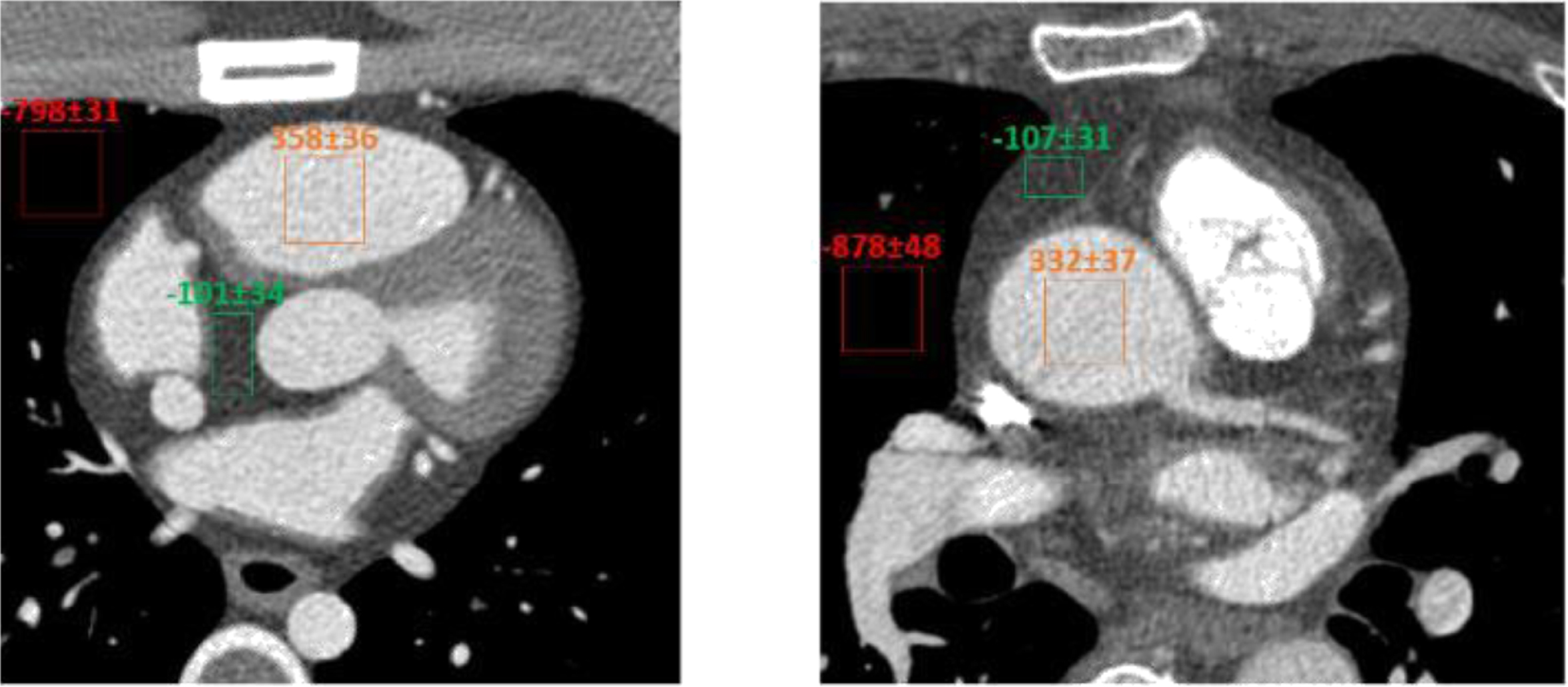
Comparison of the XCAT simulated image (left) and the real image obtained from a GE Revolution CT (right) using an axial scanning mode.

3.3 Mask method results

The reference image represents the phase most suitable for use in determining the mask region for a vessel. In this image, image processing tools are used to obtain the boundary of the organs and the regions of the organs and vessels. A convex hull is generated by combining the boundaries of vessels and organs. Then, the outside pixels of this convex hull are removed, and the inside pixels are assigned to a mask. Figure 4 illustrates this process applied to the LAD vessel of a female phantom, with a window size of 32. Figures 5 6 show the linear scoring results for the respective no-mask and masked cases.

Fig. 4

Illustration of the generation of a mask. From left to right, the six images are: the original image slice (showing the vessel region in the rectangular box), the extracted and magnified image patch of the vessels, the gradient image showing the boundaries of the vessels and organs in the patch, a polygon that contains all the boundaries in the patch, the binary image of the patch which has been thresholder to obtain the highest HU values, and the final polygon to serve as the mask.

Fig. 5

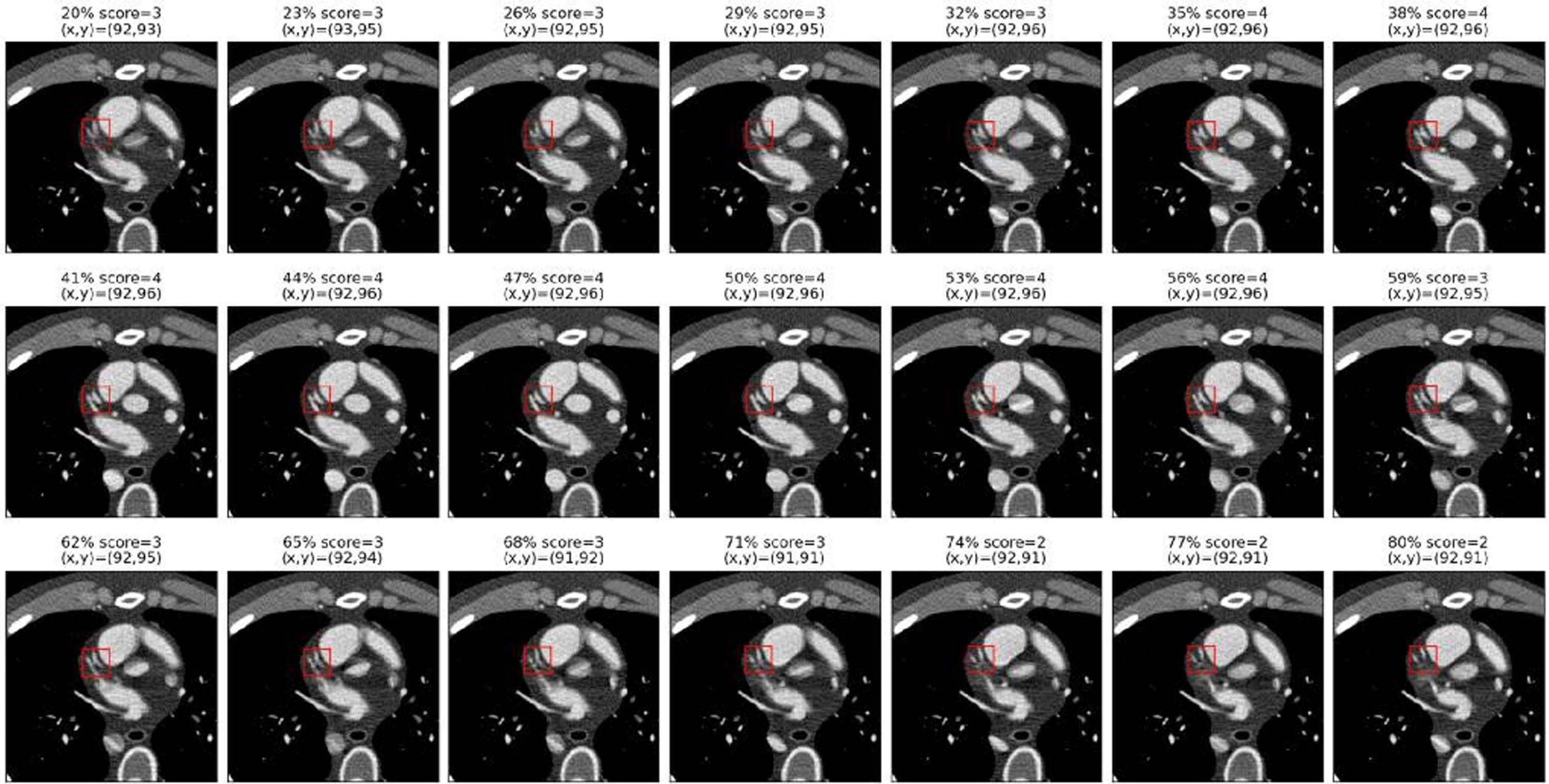
No-mask case: scoring results of a representative slice with 21 phases by using the linear score method, where (x,y) indicates the patch location.

Fig. 6

Mask case: scoring results of a representative slice with 21 phases by using the linear score method where (x,y) indicates the patch location.

We are comparing the difference between using a square window and square window with mask. From the location results, these two different windows attempt to find the region with the best SSIM value, and the results are different. For example, from the last cardiac phase in Figures 5 6, we can see the vessels are moving left and moving up; the results for the no-mask case in Fig. 5 show there is only upward, and no leftward movement; and the results in Fig. 6 show both upward and leftward motion. The reason is that a square window covers a greater organ area, and this area will dramatically affect the sliding window process. Even we use the mask method, the results are not improved much. The reason could be the background effect increase after removing the large organs. These results would likely be improved if the effect of the background were decreased.

3.4 Scoring results

In Table 2, scoring results for the LAD are compared for four different methods, where the integers are the results of each method and the decimals in parentheses are the corresponding continuous results. For the linear score method and linear method with mask, the parameters of slope and intercept are adjusted, and the sequence of SSIM values fed into the linear model to yield the continuous results. We then round to the closet integer to get the score. For k-means scores and k-means with mask scores, the sequence of SSIM values is classified into different groups, and each group represents a score. The linear scores and linear-with-mask scores tend to have similar results, but there is a difference in phase 32.

Table 2
Examples of using linear score, linear-score-with-mask, k-means score and k-means-score-with-mask

LAD phase 20 23 26 29 32 35 38 41 44 47 50

Linear score 3(2.60) 3(2.79) 3(2.99) 3(3.22) 3(3.47) 4(3.57) 4(3.65) 4(3.69) 4(3.74) 4(3.80) 4(3.69)

Mask score 3(2.65) 3(2.85) 3(3.04) 3(3.27) 4(3.51) 4(3.60) 4(3.67) 4(3.71) 4(3.75) 4(3.80) 4(3.71)

k-means score 3 3 3 3 4 4 4 4 4 4 4

Mask with k-means 3 3 3 3 4 4 4 4 4 4 4

Average score 3(2.81) 3(2.91) 3(3.00) 3(3.12) 4(3.75) 4(3.79) 4(3.83) 4(3.85) 4(3.87) 4(3.90) 4(3.85)

LAD phase 53 56 59 62 65 68 71 74 77 80

Linear score 4(3.63) 4(3.54) 3(3.41) 3(3.16) 3(2.86) 3(2.75) 3(2.50) 2(2.24) 2(1.96) 2(1.80)

Mask score 3(3.66) 4(3.59) 3(3.47) 3(3.23) 3(2.96) 3(2.79) 3(2.54) 2(2.28) 2(1.99) 2(1.80)

k-means score 4 4 4 3 3 3 3 2 2 2

Mask with k-means 4 4 4 3 3 3 3 2 2 2

Average 4(3.82) 4(3.78) 4(3.72) 3(3.10) 3(2.96) 3(2.89) 3(2.76) 2(2.13) 2(1.99) 2(1.88)

LAD phase	20	23	26	29	32	35	38	41	44	47	50
Linear score	3(2.60)	3(2.79)	3(2.99)	3(3.22)	3(3.47)	4(3.57)	4(3.65)	4(3.69)	4(3.74)	4(3.80)	4(3.69)
Mask score	3(2.65)	3(2.85)	3(3.04)	3(3.27)	4(3.51)	4(3.60)	4(3.67)	4(3.71)	4(3.75)	4(3.80)	4(3.71)
k-means score	3	3	3	3	4	4	4	4	4	4	4
Mask with k-means	3	3	3	3	4	4	4	4	4	4	4
Average score	3(2.81)	3(2.91)	3(3.00)	3(3.12)	4(3.75)	4(3.79)	4(3.83)	4(3.85)	4(3.87)	4(3.90)	4(3.85)
LAD phase	53	56	59	62	65	68	71	74	77	80
Linear score	4(3.63)	4(3.54)	3(3.41)	3(3.16)	3(2.86)	3(2.75)	3(2.50)	2(2.24)	2(1.96)	2(1.80)
Mask score	3(3.66)	4(3.59)	3(3.47)	3(3.23)	3(2.96)	3(2.79)	3(2.54)	2(2.28)	2(1.99)	2(1.80)
k-means score	4	4	4	3	3	3	3	2	2	2
Mask with k-means	4	4	4	3	3	3	3	2	2	2
Average	4(3.82)	4(3.78)	4(3.72)	3(3.10)	3(2.96)	3(2.89)	3(2.76)	2(2.13)	2(1.99)	2(1.88)

In Table 3, we compare the average automatically-calculated (machine) scores with human reader scores. The average score is computed by averaging two continuous scores of linear and linear-with-mask and the two integer scores of non-linear methods. From the results, we can see the difference between average score and reader score is small for all phases. In phases 32, 56 and 59, the machine score averages are greater than the reader score, because the k-means method yields higher scoring results.

Table 3

Example of comparison between average score and real score

LAD phase	20	23	26	29	32	35	38	41	44	47	50
Average score	3(2.81)	3(2.91)	3(3.00)	3(3.12)	4(3.75)	4(3.79)	4(3.83)	4(3.85)	4(3.87)	4(3.90)	4(3.85)
Human reader score	3	3	3	3	3	4	4	4	4	4	4
LAD phase	53	56	59	62	65	68	71	74	76	80
Average score	4(3.82)	4(3.78)	4(3.72)	3(3.10)	3(2.96)	3(2.89)	3(2.75)	2(2.13)	2(1.99)	2(1.88)
Human reader score	4	3	3	2.5	2.5	2.5	2.5	2.5	3	3

The experiment results on evaluating the scoring method on the synthetic images data is shown in Table 4. We compare the mean squared error between linear scores and k-means scores, with and without a mask, on the RCA, LAD, and LCX synthetic images by using the results in the Tables 2 3, which have 21 images. All methods exhibit low error rates relative to the reader scores. The linear model tends to yield smaller errors, since it provides continuous scores, whereas the k-means method always gives integer scores. Therefore, when errors are small, the coarse granularity of the k-means method can lead to larger apparent errors when interpreting the score.

Table 4

Evaluation of four different methods on the RCA, LAD, LCX using mean squared error of the score

Mean square error	RCA	LAD	LCX
Average	0.834	0.244	0.813
Linear	0.610	0.239	0.733
Linear with mask	0.657	0.247	0.685
k-means	1.011	0.297	0.964
k-means with mask	1.297	0.297	0.964

3.5 Deep learning-based classification results

Networks are trained separately for each vessel (LAD, LCX, RCA) since the characteristics of these vessels is different. The quantitative analysis results appear in Table 5, where L₁ represents the mean of absolute differences between the true value and the predicted value (i.e., the L₁ loss). The mean square error is also used as a metric to evaluate the performance. After the synthetic images are generated by the XCAT software and labeled by the semi-auto labeling method, they are added to the training dataset for neural network training. As shown in Table 5, compared with the results using real data only, the L₁ loss and mean square error decrease when adding the generated data into the training dataset. If the synthetic dataset alone is used for training, and real images are used for testing, we find even greater L₁ loss and MSE loss. We thus conclude that these simulated data are useful and effective when they are added into a real dataset.

Table 5
Performance comparison of different training strategies for neural network

Vessel Real data without simulated data Real data with simulated data Simulated data only

RCA L₁ = 0.5802, MSE = 0.6015 L₁ = 0.5802, MSE = 0.3874 L₁ = 0.4503, MSE = 1.0696

LAD L₁ = 0.4429, MSE = 0.3747 L₁ = 0.4230, MSE = 0.3588 L₁ = 0.9156, MSE = 1.1232

LCX L₁ = 0.5164, MSE = 0.4462 L₁ = 0.5066, MSE = 0.4366 L₁ = 0.8058, MSE = 0.9677

Vessel	Real data without simulated data	Real data with simulated data	Simulated data only
RCA	L₁ = 0.5802, MSE = 0.6015	L₁ = 0.5802, MSE = 0.3874	L₁ = 0.4503, MSE = 1.0696
LAD	L₁ = 0.4429, MSE = 0.3747	L₁ = 0.4230, MSE = 0.3588	L₁ = 0.9156, MSE = 1.1232
LCX	L₁ = 0.5164, MSE = 0.4462	L₁ = 0.5066, MSE = 0.4366	L₁ = 0.8058, MSE = 0.9677

4 Discussion

In this paper, we use a sliding window with different kernel and window sizes to locate moving coronary vessels. The sliding window, however, contains significant background anatomy. To remove some of the influence of background we implement a mask method. However, the mask region is still greater than the ideal vessel region-of-interest, and the background area will thus still affect the SSIM values and the label results. Methods could be developed to determine a more precise region and further attenuate the background effect.

The second step is to score the vessels for motion artifact. Both the linear and k-means methods are used. The auto-labeling results strongly agree with the expert reader-assigned scores. For the linear scoring method, the mean squared errors for RCA, LAD and LCX are 0.610, 0.239, and 0.733, respectively. The RMS errors are thus all less than one score point. If we consider the top-1 error, this error is much smaller. This implies that the assigned labels are reasonable and that the image quality is strongly accords with expert opinion. These results imply that synthetic XCAT images with auto-semi labeling process can generate valuable datasets to supplement real image datasets for network training, since these can further improve the performance of the network. Since there exists non-linearity between SSIM values and score results (for example, in phases 77 and 80 [shown in Figs. 5 6]), even though the SSIM values are low, the reader scores for these phases are higher because the vessels appear more prominent. In future work, we will attempt to remedy this by including more features in non-linear scoring methods. For example, using more precisely segmentation method to locate vessel’s position will increase the performance. Many researchers are working on improved techniques for the automatic segmentation of the cardiac boundaries [24, 25].

When the neural network was applied to the same regression task, the maximum mean square errors over all artery types, when trained on simulated, real, and real+simulated data were 1.1232, 0.6015 and 0.4366, respectively (Table 5). The network thus performed best for the simulation-supplemented real data and achieved a worst-case RMS error of less than 0.7 points.

5 Conclusion

We have demonstrated that coronary motion phase estimation algorithms on accord with expert opinion within 0.85 scoring points (RMS) on a 5-point scale. Such methods can be used to score coronary artery image quality at exam time and can thus indicate whether a scan is of sufficient clinical quality, as well as automatically identify the most diagnostically useful imaging phases. Patient throughput is important to reduce healthcare costs and increase convenience to patients and staff at radiology clinics. Tools that automate fundamental image quality analysis while the patient is in situ can avoid requiring a patient to return for a repeat scan after a radiologist (who would generally read the scan after the patient has departed the radiology facility) has determined the scan is deficient. This can lead to increases in convenience and patient throughput, as well as patient outcomes in time-sensitive cases.

We have also demonstrated the utility of supplementing real training data with realistic phantom data for increasing network performance and decreasing the amount of clinical data required for training. This is significant, since the availability of large enough clinical datasets to reliably train a network that is not biased by selection of too narrow a sample of anatomic variation is the main barrier to high performance medical imaging AI. Further investment in realistic digital phantom representations of normal anatomy and pathology would thus likely have the potential to increase the scope and performance of clinical AI.

Footnotes

Acknowledgments

This work was funded by GE Healthcare.

References

Anderson

K.M.

, Odell

P.M.

, Wilson

P.W.F.

and Kannel

W.B.

, Cardiovascular disease risk pro les, American Heart Journal 121(1) (1991), 293–298.

Tardif

J.C.

, , Coronary artery disease in, European Heart Journal Supplements 12(suppl C) (2010), C2–C10.

Haase

, Schlattmann

, Gueret

, et al., Diagnosis of obstructive coronary artery disease using computed tomography angiography in patients with stable chest pain depending on clinical probability and in clinically important subgroups: meta-analysis of individual patient data, BMJ (2019), 365, Article ID: l1945, 2019.

SCOT-Heart Investigators, Coronary CT angiography and 5-year risk of myocardial infarction, New England Journal of Medicine 379(10) (2018), 924–933.

Hausleiter

, Meyer

, Hermann

, et al., Estimated radiation dose associated with cardiac CT angiography, JAMA 301(5) (2009), 500–507.

Kalra

M.K.

, Maher

M.M.

, Toth

T.L.

, et al., Strategies for CT radiation dose optimization, Radiology 230(3) (2004), 619–628.

Richards

C.E.

, Dorman

, John

, et al., Low-radiation and high image quality coronary computed tomography angiography in “real-world” unselected patients, World Journal of Radiology 10(10) (2018), 135–142.

Dey

, Slomka

P.J.

and Berman

D.S.

, Achieving very-low-dose radiation exposure in cardiac computed tomography, single-photon emission computed tomography, and positron emission tomography, Circulation: Cardiovascular Imaging 7(4) (2014), 723–734.

Brenner

D.J.

and Hall

E.J.

, Computed tomography an increasing source of radiation exposure, New England Journal of Medicine 357(22) (2007), 2277–2284.

10.

Kim

, Chang

and Ra

J.B.

, Cardiac motion correction based on partial angle reconstructed images in x-ray CT, Medical Physics 42(5) (2015), 2560–2571.

11.

Sun

, Kim

J.H.

, Fulton

and Nuyts

, An iterative projection-based motion estimation and compensation scheme for head x-ray CT, Medical Physics 43(10) (2016), 5705–5716.

12.

Jang

, Kim

and Ra

J.B.

, Head motion correction based on filtered back projection for x-ray CT imaging, Medical Physics 45(2) (2018), 589–604.

13.

Zeleznik

, Foldyna

, Eslami

, et al., Deep convolutional neural networks to predict cardiovascular risk from computed tomography, Nature Communications 12(1) (2021), Article Number:715, pp. 9.

14.

Litjens

, Ciompi

, Wolterink

J.M.

, et al., State-of-the-art deep learning in cardiovascular image analysis, JACC: Cardiovascular Imaging 12(8 Part 1) (2019), 1549–1565.

15.

Chlap

, Min

, Vandenberg

, et al., A review of medical image data augmentation techniques for deep learning applications, Journal of Medical Imaging and Radiation Oncology 65(5) (2021), 545–563.

16.

Wolterink

J.M.

, van Hamersvelt

R.W.

, Viergever

M.A.

, et al., Coronary artery centerline extraction in cardiac CT angiography using a CNN-based orientation classifier, Medical Image Analysis 51 (2019), 46–60.

17.

Chen

, Qin

, Qiu

, et al., Deep learning for cardiac image segmentation: a review. Frontiers in Cardiovascular Medicine, Vol. 7, Article Number: 25, 2020.

18.

Seemann

, Bargsten

and Schlaefer

, Data augmentation for computed tomography angiography via synthetic image generation and neural domain adaptation, Current Directions in Biomedical Engineering 6(1) (2020), Article ID: 20200015.

19.

Sandfort

, Yan

, Pickhardt

P.J.

and Summers.

R.M.

, Data augmentation using generative adversarial networks (cyclegan) to improve generalizability in CT segmentation tasks, Scientific Reports 9(1) (2019), Article number: 16884.

20.

Frangi

A.F.

, Tsaftaris

S.A.

and Prince

J.L.

, Simulation and synthesis in medical imaging, IEEE Transactions on Medical Imaging 37(3) (2018), 673–679.

21.

Wang

, Bovik

A.C.

, Sheikh

H.R.

and Simoncelli

E.P.

, Image quality assessment: from error visibility to structural similarity, IEEE Transactions on Image Processing 13(4) (2004), 600–612.

22.

Segars

W.P.

, Sturgeon

, Mendonca

, et al., 4D XCAT phantom for multimodality imaging research, Medical Physics 37(9) (2010), 4902–4915.

23.

, Zhang

, Ren

and Sun

, Deep residual learning for image recognition. CoRR, abs/1512.03385, 2015.

24.

Zheng

, Barbu

, Georgescu

, et al., Four-chamber heart modeling and automatic segmentation for 3-D cardiac CT volumes using marginal space learning and steerable features, IEEE Transactions on Medical Imaging 27(11) (2008), 1668–1681.

25.

Peng

, Lekadir

, Gooya

, et al., A review of heart chamber segmentation for structural and functional analysis using cardiac magnetic resonance imaging, Magnetic Resonance Materials in Physics, Biology and Medicine 29(2) (2016), 155–195.