
Abstract
BACKGROUND:
Beam-hardening in tomography with polychromatic X-ray sources results from the nonlinear relationship between the amount of substance in the X-ray beam and attenuation. Simple linearisation curves can be derived with the use of an appropriate step wedge, however, this does not yield good results when different materials are present whose relationships between X-ray attenuation and energy are very different.
OBJECTIVE:
To develop a more accurate method of beam-hardening correction for two-phase samples, particularly immersed or embedded biological hard tissue.
METHODS:
Use of a two-dimensional step wedge is proposed in this study. This is not created physically but is derived from published X-ray attenuation coefficients in conjunction with a modelled X-ray spectrum, optimised from X-ray attenuation measurements of a calibration carousel. To test this method, a hydroxyapatite disk was scanned twice; first dry, and then immersed in 70% ethanol solution (commonly used to preserve biological specimens).
RESULTS:
With simple linearisation the immersed disk reconstruction exhibited considerable residual beam hardening, with edges appearing approximately 10% more attenuating. With 2-dimensional correction, the attenuation coefficient showed only around 0.5% deviation from the dry case.
CONCLUSION:
Two-dimensional beam-hardening correction yielded accurate results and does not require segmentation of the two phases individually.
Introduction
When a polychromatic X-ray beam is attenuated by an object, lower-energy X-rays are generally more highly attenuated, resulting in a filtering effect which increases the mean energy of the beam. In computed tomography, this leads to dishing artefacts, whereby scanned objects appear to be less dense toward the centre. Beam hardening correction aims to compensate for this effect, thus reducing these artefacts [1]. Herman [2] describes this as follows: “We investigate how one can estimate from the total attenuation, p, of a polyenergetic X-ray beam what the total attenuation, m, of a monoenergetic beam would have been along the same ray”. Herman showed that a set of polychromatic projections could be linearised using a simple polynomial to produce a good approximation of monochromatic projections for the purpose of obtaining reasonably accurate CT numbers; certainly more accurate that would have been obtained without such linearisation. A reasonable approximation can often be made with a 2nd order polynomial. Since the curve passes through the origin, the constant term is zero. With X-ray microtomography (XMT or micro-CT), it is often unnecessary to reproduce an absolute linear attenuation coefficient, especially where structure is of primary importance. The linear term can therefore be fixed, leaving only the 2nd order term, which can be adjusted manually to minimise the apparent beam hardening artefacts (dishing and streaking). Such an approach, however, is particularly unsuitable for the study of mineral concentration in teeth, the author’s primary interest, since dental enamel exhibits a true radial gradient in mineral concentration which is difficult to distinguish from the apparent dishing in density resulting from beam hardening. Therefore, a beam hardening correction method that does not depend on subjective assessment is necessary.
Step wedges have long been used to linearise X-ray attenuation [3] and can thus be used for beam hardening correction. Because the relationship between X-ray energy and attenuation for a given material depends on its composition, it is necessary that the step wedge be representative of the object being scanned. For example, a step wedge made from a hydroxyapatite (HA) and epoxy resin composite has been used to represent bone [4]. The ability to make such a representative step wedge will depend on the physical properties of the material in question, with the material chosen as a compromise between its physical and X-ray properties. The Queen Mary University of London (QMUL) group proposed the indirect use of a step wedge for use in their XMT scanner, whereby attenuation measurements from the step wedge were used to optimise a model of the X-ray spectrum [5]. Using published X-ray attenuation values [6], a virtual step wedge was created from the modelled spectrum and this was used to create the linearization curve (expressed as a polynomial). For practical reasons, the aluminum step wedge was later replaced with a multi-element carousel [7] which was permanently mounted under the rotation stage of the XMT scanner such that attenuation measurements could be recorded with every scan (a similar, open-source method has also been published [8]). Such frequent calibration is necessary because of shifts in the X-ray spectrum with time, principally due to pitting of the X-ray target (in the case of reflection targets). The calibration software used at QMUL also accounts for variation in the X-ray spectrum with image height (differences in measured attenuation of approximately 5 % were recorded between the top and bottom of the detector owing to the difference in X-ray take-off angle). Although primarily designed for use in the study of biological hard tissue, this modelling method was also found to work for a number of different materials [9] (aluminum, sulfur, titanium and potassium iodide solution were tested).
XMT has been used in the study of mineral concentration in teeth since it was first described [10]. Using such methods, it is possible to quantify the loss of mineral that occurs during acid attack and to investigate the effects of therapeutic agents that attempt to restore this mineral. Densitometric accuracy is of paramount importance in this type of research, which requires images with a good signal-to-noise ratio (SNR) and minimal systematic errors. Time-delay integration scanners were designed for this purpose at QMUL [11, 12], which are free from ring artefacts and many other systematic errors, facilitating long exposures to obtain a high signal-to-noise ratio (SNR). The calibration carousel with an HA virtual step wedge was considered to provide accurate quantitative results for dry teeth. However, to prevent dehydration, teeth often need to be stored and scanned in solution (typically 70 % alcohol, commonly used to preserve biological specimens), or sometimes in demineralising or remineralising solutions in dynamic studies. In such cases, even though X-ray attenuation was dominated by the mineral component of the teeth (principally owing to the high atomic number of calcium compared with elements in the organic tissue, solution, or plastic container), beam hardening appeared to be under-corrected when using the virtual step-wedge approach. Occasionally, the measured linear attenuation coefficient (LAC) on the outer edges of enamel exceeded that expected for 100 % HA, which is clearly an erroneous result. To reduce such errors, it was necessary to employ a beam-hardening correction method that considers the presence of two phases with different X-ray attenuation properties.
Methods
General principle
Many methods for dual- or multi-phase beam-hardening correction have been described, but these tend to rely on segmentation of the separate phases in an initial reconstruction [13–15]. Such methods assume that the phases are mutually exclusive, at least at the detected resolution. However, teeth contain varying proportions of mineral and organic phases; thus, it is not possible to separate the two using segmentation since each voxel may represent a mixture of both phases. For simplicity, we consider there to be just two phases: a mineral phase and an organic phase, the latter representing soft tissue, any immersion or embedding media, and a plastic container, if present. Such a simplification is appropriate when we are not concerned primarily with quantification of the LAC of any of these “organic” components, but rather their effect on the quantification of the mineral phase. Furthermore, we assume, though unresolvable, that these phases are mutually exclusive; that is, that the mineral (M) phase displaces its own volume of the organic (O) phase. It is therefore possible to divide the phases into the O-phase and a difference phase (D), whose linear attenuation coefficient is that of the M-phase minus the O-phase. Although this technique can be applied to embedded samples of any shape, we considered only the case of an immersed sample in a plastic container with a circular cross-section and a possible taper (typical sample containers have a slight taper). Within the liquid level of this container, the entire sample was considered to be a 100% O-phase coincident with a variable amount of the D phase. It is then unnecessary to segment the M-phase in an initial reconstruction, but only the O-phase, which is a trivial matter of identifying the outer surface of the container.
For beam-hardening correction, a two-dimensional virtual step-wedge is modelled, with X-ray attenuation as a function of both the amount of O- and D-phases in the beam. A 2-D polynomial is fitted to yield the equivalent monochromatic attenuation of the D phase as a function of the measured attenuation and the amount of O-phase, as determined from its segmentation. This D-phase attenuation was then added to the modelled O-phase attenuation prior to reconstruction. Although the D-phase could be reconstructed directly, any error resulting from differences in the O-phase composition would directly affect the result; here, the effect of O-phase composition on the M-phase quantification is much smaller, and the LAC of the O-phase can be measured from the reconstruction.
A single X-ray projection from a typical tooth (immersed in a 17 mm diameter plastic container of 70% ethanol solution) is shown in Fig. 1. Figure 1a shows the raw polychromatic projection, b shows the modelled O-phase derived from an initial reconstruction, c shows the D-phase and d shows the summed equivalent monochromatic (corrected) projection. Note that in each of these, the grayscale is normalised. The attenuation along a line profile, indicated by the dotted line in 1a, is shown in Fig. 2.
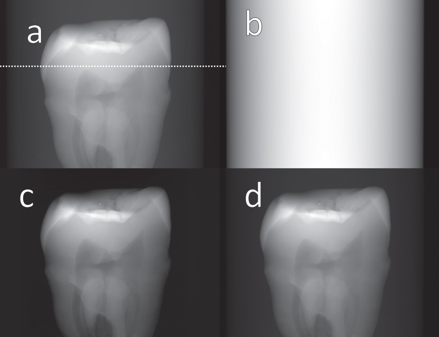
Single X-ray projection from a typical immersed tooth scan. (a) Raw polychromatic projection. (b) Modelled O-phase. (c) D-phase (difference between inorganic and organic phases). (d) Summed equivalent monochromatic (corrected) projection. Note that in each of these, the grayscale is normalised. Attenuation along a line profile, indicated by the dotted line in (a) is shown in Fig. 2.
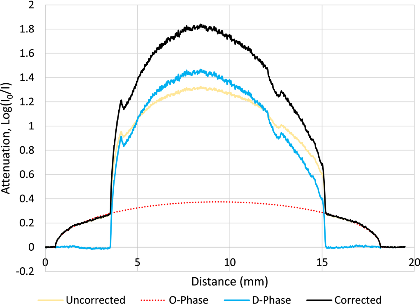
Attenuation through a typical immersed tooth X-ray projection along the dotted line of Fig. 1a.
The MuCat 2 scanner is an in-house design that employs time-delay integration to eliminate ring artefacts. The scanner contains a 225 kV X-ray source from X-tek (Nikon Metrology Uk Ltd), containing a cylindrical anode (reflection target) with its axis horizontal. A CsI scintillator is coupled, via a low-distortion fiber-optic faceplate, to a 16 Megapixel 6 cm square CCD. The camera is translated along a linear motion stage perpendicular to the central ray, with the CCD rows vertical. The camera is read out constantly (in 2×2 binning mode) as it scans through the image, with a frame shift rate matching the horizontal velocity, such that the accumulating charge image is static during the exposure. In addition to immunity to ring artefacts, this has the advantage that the image width can be larger than the CCD width. The exposure time is the time taken for the CCD to travel its own width. Additional time is taken for the CCD to travel one width prior to the start of readout, for initial charge integration, and for flyback. Other components have been described elsewhere [12].
Carousel calibration
The calibration carousel comprises two 85 mm diameter, 5 mm thick duralumin disks, around which are bolted nine calibration samples, each 50 mm×12.5 mm (Fig. 3). These are made of aluminum (99.999% pure), titanium (99.6% pure), and copper (99.98% pure) from Advent Research Materials (Oxford, UK). The calibration samples comprise 0.2 mm Al, 0.5 mm Al, 1.0 mm Al, 2.0 mm Al, 4.0 mm Al, 1.0 mm Ti, 2.0 mm Ti, 4.0 mm Ti and 2.0 mm Cu, in order of increasing X-ray attenuation. The 2 and 4 mm thick samples of aluminum and titanium samples were made by stacking 1 mm sheets.
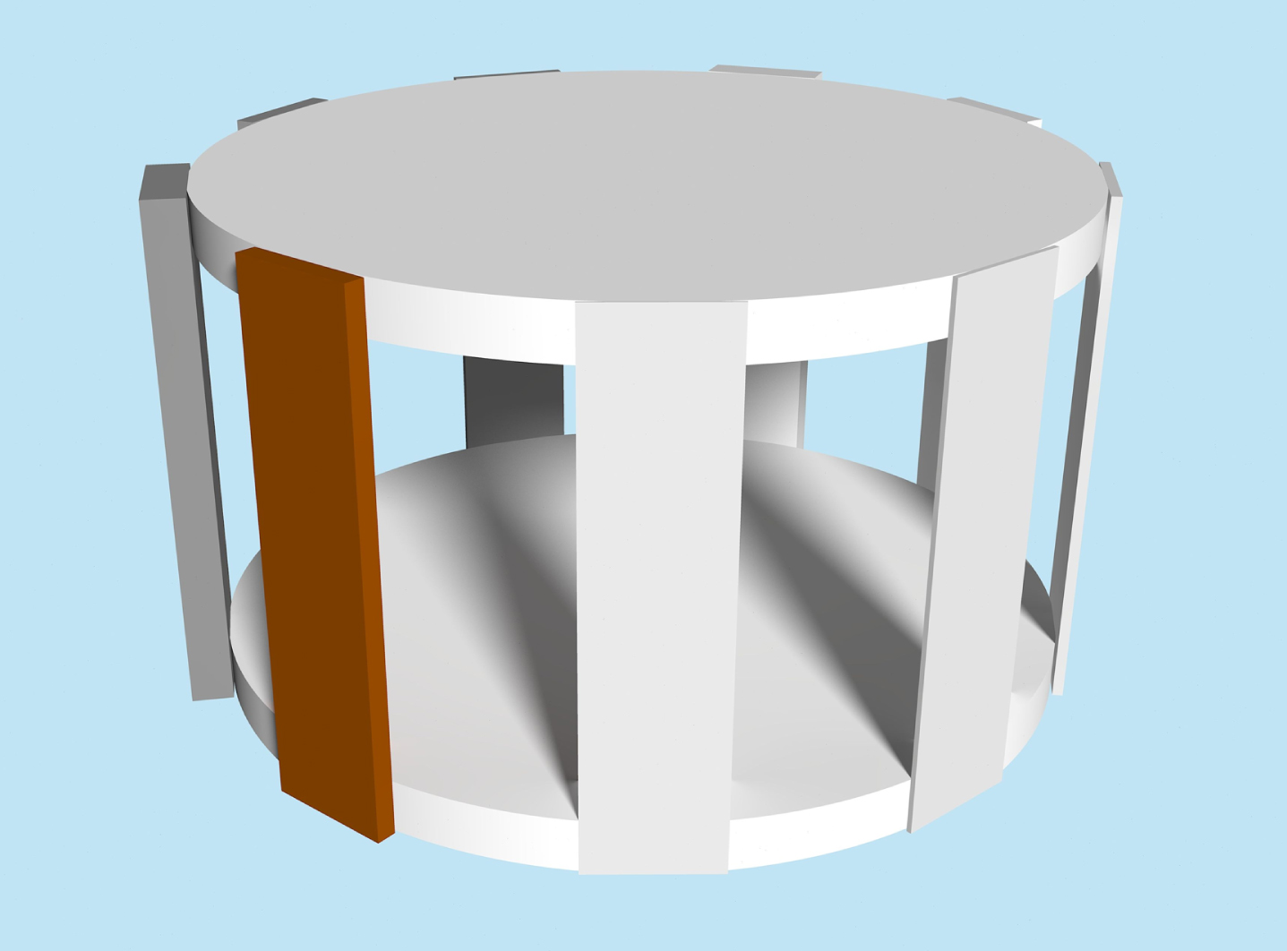
Calibration carousel comprising of two duralumin disks surrounded by calibration pieces made of aluminium, titanium and copper.
The carousel is mounted under the scanner rotation stage and is raised into the beam after each complete sample scan. The X-ray beam passes through the gap between two of the calibration samples to image the opposite sample. The carousel is mounted with its centre of rotation 81 mm from the X-ray source, meaning that the gap is approximately 38.5 mm away, whilst the sample being imaged is 123.5 mm away. The carousel is rotated in 40° steps so that all nine samples are imaged. The recorded images are 600×1000 pixels in size. These are dark and flat field corrected and divided into two 600×500 sub-images. The left and right edges of the samples are detected and the mean attenuation recorded from the central 200×500 area in each sub-image.
The spectrum is defined by five variable intensities, initially set to unity, at 12.5%, 37.5%, 62.5%, and 87.5% of the accelerating voltage. Intermediate intensities at 0.5 kV intervals are determined by linear interpolation, with zero intensity for 0 and 100% of the accelerating voltage. For most studies on extracted teeth, the voltage is set to 90 kV. The spectrum is virtually filtered with 1 mm aluminum and 50μm copper (matching that on the X-ray system when set to 90 kV) using linear attenuation values determined from published (XCOM) X-ray data [6]. Absorption by a 100μm thick caesium iodide scintillator is similarly modelled, and the light output, and hence the detected response, is assumed to be proportional to the X-ray photon energy. Attenuation values for each of the nine calibration samples are then calculated and compared with the recorded attenuation values, and the error is computed as the sum of the squared differences for all nine samples. The 37.5% energy intensity is fixed, whilst the remaining four are optimised using a simplex algorithm [16] that minimises the error. This algorithm adjusts the logarithm of intensity to ensure that it cannot be negative. This process is repeated for both sub-image sets, allowing for variation in the spectrum caused primarily by the change in take-off angle with the height at which rays intercept the detector. Virtual filtering and scintillator modelling are not strictly necessary, as the optimisation would adjust for this. However, filtering after linear interpolation yielded a spectrum closer to that which would be expected, and the error values were lower.
Virtual step-wedge
One-dimensional step-wedge
For the single-phase case, a 100-step virtual step wedge is created with linear intervals of thickness of a representative material (HA for biological hard tissue), the thickest being that required for attenuation of the X-ray spectrum, according to modelled light output, by e–6. Attenuation values for each step are calculated for every sub-image set, and the results are interpolated such that each row of the detector has an associated set of attenuation values. A monochromatic calibration energy value is selected which is approximately representative of the mean energy of the polychromatic spectrum. For a 90 kV accelerating potential, this is set to 40 keV. A set of monochromatic attenuation values for the virtual step wedge is also calculated. Seventh-order polynomials are then created by least-squares fitting for each detector row, giving monochromatic attenuation as a function of polychromatic attenuation. These are used for the linearisation of the scan data.
Two-dimensional step-wedge
For the dual-phase case, a 50×50 step virtual wedge is created with equal steps of a representative organic material in one dimension, up to that required to give attenuation by e–3. For an immersed tooth, material is generally considered to be water or 70% ethanol. In the other dimension, the virtual step wedge represents attenuation by the difference phase, whose linear attenuation coefficient is that of the mineral phase minus the organic phase (e.g. HA –70% ethanol). Thus, 2500 polychromatic attenuation values are calculated for each sub-image. A similar matrix is created for the monochromatic calibration energy. For both attenuation matrices, a 2-dimensional polynomial is fitted, giving monochromatic attenuation of the difference phase as a function of total polychromatic attenuation and monochromatic attenuation by the organic phase. The polynomial is 8th order with a constraint of a maximum 8th order in any term (e.g. x8, y8, x4y4, etc.). This was found to yield better results than a 6th order unconstrained polynomial [17] (higher orders yield unpredictable errors). By interpolation, 1000 polynomials (one for every image row) are derived from the upper and lower sub-image polynomials.
Application of the two-dimensional polynomial
The current implementation of this algorithm is limited to specimens immersed in near-cylindrical (conical, circular cross section with a slight taper) containers. In theory, any shaped container can be implemented, but it should be noted that corrections can only be made for X-ray projections that fully intercept the reconstructed volume. The advantage of the near-cylindrical constraint is that this shape can be extrapolated vertically; otherwise, the top and bottom of the projections cannot be beam hardening corrected using this method because the shape of the O-phase outline would not be known in these regions owing to the beam divergence. An initial reconstruction is performed without beam hardening correction. It is assumed that the container is mounted nearly vertically, that is, with its central axis nearly parallel to the rotation axis; thus, the cross section can be approximated as a circle. A circle is fitted to the outline of the container in every slice of the reconstruction, recording its centre coordinates and radius. Straight lines are fitted to the coordinates and radius after eliminating any that fall outside 5% of the median. As part of the initial reconstruction process, the intercept of the centre of rotation on the projection is determined. Using this, the fitted cone parameters, and the known monochromatic linear attenuation coefficient of the O-phase at the calibration voltage, the O-phase is forward-projected to create a set of projections with geometry matching that of the scanner. This and the original attenuation projections constitute the two inputs to the polynomial to yield the D-phase monochromatic projections. This is added to the O-phase prior to reconstruction.
Summary of algorithm steps
The steps in the 2D beam-hardening correction, assuming a sample immersed in a container of 70% ethanol solution, are as follows: Scan the sample Scan the calibration carousel. Reconstruct the sample with simple or no beam hardening correction. Segment the container and fit a conical surface (modelling a typical sample container). Calculate the path length for all projections through the container assuming it is filled with 70% ethanol solution (use the centre-of-rotation derived in the reconstruction process). Derive a modelled X-ray spectrum optimised from the carousel attenuation values (this is a function of height as it varies with X-ray take-off angle). Separate spectra are calculated for the upper and lower halves of the image Derive a virtual 2-dimensional step-wedge for the ‘O’ and ‘D’ phases Calculate attenuation through the two-dimensional step-wedge and derive from this a 2-dimensional polynomial for expected monochromatic attenuation of the ‘D’ phase as a function of measured polychromatic attenuation and path-length through the container. This is done for the upper and lower spectra and then interpolated for every row of the image. Using the polychromatic projections and path-length projections, apply the polynomial (for each image row) to calculate the set of monochromatic ‘D’ phase projections. Derive the monochromatic ‘O’ phase projections as the product of the theoretical LAC of the solution and the projected path lengths. Add the ‘O’ and ‘D’ phase projections to produce the corrected projections Perform the final reconstruction
Shortcomings and compensation
Although the spectrum optimisation converged, the modelled versus real attenuation of the calibration samples showed discontinuities between the different metals. This could not be accounted for by deviations in the thicknesses of the samples and is unlikely to have been due to impurities (the titanium was only 99.6% pure). The most probable cause is X-ray scattering, which was not modelled. Without the complex task of scatter modelling, the options were to use the best fit with the discontinuities or make a phenomenological adjustment (one that has no physical basis) to the model. The latter option was chosen, and the thicknesses of the calibration samples in the model were adjusted away from their true values. This adjustment was made in a systematic manner. A separate thickness factor was considered for each material (Cu, Ti and Al). The Ti thickness was initially set to 1.0, and an optimisation algorithm adjusted the Cu and Al thickness factors to minimise the error in the optimised model (optimisation within optimisation). A 10 mm diameter 99.999% pure Al rod was scanned with a 15μm voxel size at 90 kV with 1917 projections over 360°. This was selected as being typical of the size and attenuation of a tooth sample. The mean LAC of the reconstructed rod was measured and compared to the expected value. The Ti thickness factor was then manually adjusted, and the entire process was repeated until the reconstructed LAC matched the expected value. The adjusted calibration sample thicknesses were retained for future use; it was not necessary to repeat this nested optimisation process. However, for immersed samples, the X-ray scatter is increased, and thus, these values are no longer optimal. Therefore, the Al rod was re-scanned immersed in 70% ethanol solution in the same type of sample container used for tooth samples. The nested optimisation process was repeated to obtain a set of thicknesses to be used in conjunction with immersed samples.
Test methodology
To test the methodology, an 11 mm diameter, 3.7 mm thick sintered HA disk (approximately 5% porous) was scanned. The X-ray generator was set to 90 kV and 180μA, with a 15μm voxel size and 1215 projections over 360°. This was initially scanned dry, and then immersed in 70% ethanol solution in a polystyrene sample container having a 17 mm external diameter. Because of the limited thickness of the disk compared to a human tooth, the latter scan was performed with it in the centre of a stack of five disks. Both scans were individually calibrated using the carousel. For the dry sample, a linearisation curve was generated from the optimised spectral model using the previously derived thicknesses for the model calibration pieces. Reconstruction was performed using filtered backprojection under Windows 10 [18]. The immersed disk with the same linearisation curve was used for one reconstruction, and a 2D linearisation curve was generated for another reconstruction of the same data (using calibration piece model thicknesses optimised for immersed samples). Linearised projections represented the expected attenuation with 40 keV monochromatic radiation.
Results
Carousel attenuation measurements
Attenuation measurements for the carousel following the calibration measurement are shown in Fig. 4. The bottom line represents 0.2 mm Al; above this 0.5 mm Al, and so on up until 2 mm Cu. Vertical height on the detector was converted to angular divergence from the centre in degrees. The dots represent the vertical centre of 10 sub-images (10 measurements made from each calibration piece). Measurements from the top of the calibration pieces are approximately 5% higher than those at the bottom. Note, that the relationship between attenuation and height is approximately linear, hence only two sub-images are used to derive the calibration polynomials.
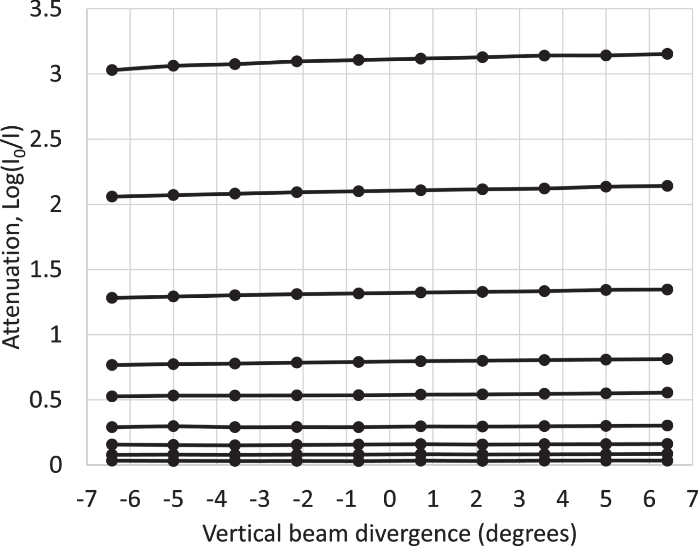
Attenuation of the test pieces at 90 kV. From bottom to top: 0.2 mm Al, 0.5 mm Al, 1 mm Al, 2 mm Al 4 mm Al, 1 mm Ti, 2 mm Ti, 4 mm Ti, 2 mm Cu.
The aluminum rod reconstructions were re-aligned to be parallel to the vertical (z) axis, and 760 slices were binned together into a single slice. Despite this averaging, a line profile through the resultant circle showed structure that could not be accounted for by noise. It is not certain whether there are real density variations within the aluminum or whether the observed structure in the reconstruction is the product of interference patterns created by the grain boundaries. Nevertheless, as seen in Fig. 5, this profile is approximately flat and free from any dishing artefact for both the standalone case and the immersed rod.
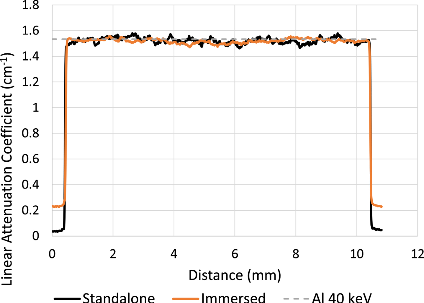
Line profile through reconstructed aluminium rod, both dry and immersed in 70% ethanol solution.
Table 1 lists the nominal and modelled thicknesses for the calibration pieces. For both the non-immersed and immersed cases, only a small adjustment was made to the copper and aluminum thicknesses. However, adjustments of approximately 10% were made for the titanium, which is too high to be accounted for by impurities and is likely the result of scatter.
Model carousel thicknesses, optimised for 10 mm Al rod reconstruction when scanned alone and immersed
The reconstructed image of the immersed disk was aligned with the image of the dry disk using an in-house 7 degree of freedom alignment procedure. A central slice of the reconstructions can be seen in Fig. 6. Here, it can be seen that there is good agreement between the image of the dry disk and of the wet disk when reconstructed with 2D beam-hardening correction. However, the reconstruction with 1D correction (simple linearisation) exhibits residual dishing as seen by the increased intensity around the edge. A “line” profile was obtained across the centre of the HA disk. To reduce the effect of random noise, the “line” was actually a cylinder of radius 10 voxels (150μm), thus each value in the profile was an average taken from a circle perpendicular to the line direction. The LAC values were converted to mineral (M-phase) concentrations (density in the dry case and partial density for the immersed sample). For the dry sample, the linear attenuation coefficient was divided by the published mass attenuation coefficient for HA at 40 keV. For the immersed sample, the following equation was used:
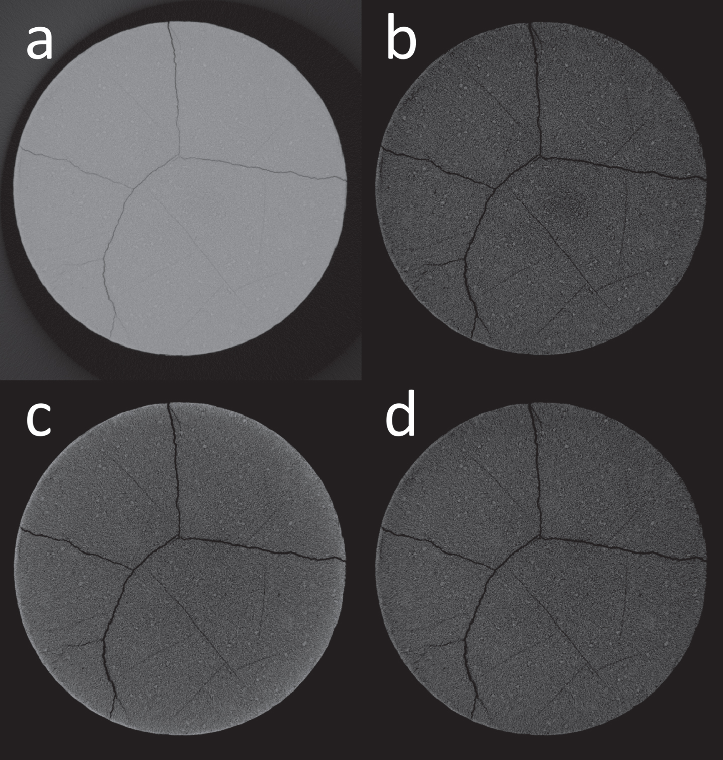
Slice view of the reconstructed HA disk; in (b), (c) and (d), the contrast has been increased by a factor of 4 to highlight subtle variations in measured perceived density. (a) and (b) Dry scan. (c) Immersed scan with 1D correction. (d) Immersed scan with 2D correction.
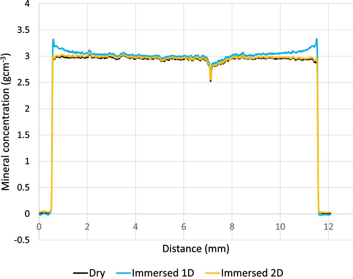
Line profiles (converted to mineral concentration) through reconstructed dry HA disk and the same disk immersed in 70% ethanol solution, both with simple 1D linearisation and 2D beam-hardening correction.
where c is the mineral concentration, μ is the measured LAC μO is the measured LAC of the organic phase (taken as a mean from a region within the container but away from the sample). μS is the published LAC for the sample material (HA in this case) ρS is the published density for the sample material (3.16 gcm–3 for HA).
The results are plotted in Fig. 6. When the linearisation curve derived for the dry disk was used with the immersed disk scan, a considerable beam-hardening artefact was observed with mineral densities being up to 10% too high at the edges, demonstrating the unsuitability of a single linearisation curve in this case. The 2D corrected reconstruction, by comparison, follows the dry case closely and is approximately 0.5% too high across the disk. This is within the expected repeatability of the calibration [9], so that is as good as could be expected.
The method of two-dimensional beam-hardening correction is applicable to cases where an easily segmented volume can be considered as containing varying fractions of two phases, the sum of which is always one. When a single linearisation curve is used to correct for beam hardening in scans of immersed tooth or bone samples, the differing X-ray attenuation properties of the organic and inorganic phases render an accurate solution impossible. The two-dimensional approach has been demonstrated to yield superior results. The scatter compensation employed in this study is not ideal and can probably be improved. Adjustments to the model were based on a 10 mm aluminum rod, which was considered to result in a similar amount of scattered radiation reaching the detector as a typical tooth scan. This may not be applicable for more attenuating samples, and further sets of adjusted thickness values should be made for different scenarios. For example, changing the resolution will change the sample-to-detector distance and thus alter the amount of scattered radiation detected. Differing X-ray acceleration potentials also require different sets of adjustments. Ongoing research by the author will focus on scatter reduction by means of anti-scatter slits in conjunction with equiangular time-delay integration scanning, whereby the sample is moved in an arc through the X-ray beam during camera readout (rather than the camera moving), averaging out any horizontal inhomogeneities in the X-ray beam. The method presented here represents the most accurate methodology known to the author for mapping mineral concentration in immersed biological hard-tissue specimens using micro-CT with a polychromatic source.
Conclusion
Although the methodology has been refined for a specific dental research application, it can be adapted to other areas. Some of the general principles can be applied, either individually or collectively. These include the basic concept of creating a two-dimensional linearisation curve and the division into a single phase with a “difference” phase to facilitate simple segmentation (as opposed to two distinct phases which may not be separable). The method is more suited to micro-CT, where a lower proportion of X-rays are scattered compared with CT at a larger scale.
Footnotes
Acknowledgments
This work made use of computational support by CoSeC, the Computational Science Centre for Research Communities, through the Collaborative Computational Project in Tomographic Imaging (CCPi). Scans on the MuCAT 2 facility at QMUL were performed by David Mills. This research did not receive any specific grant from funding agencies in the public, commercial, or not-for-profit sectors.
Conflict of interest statement
The author declares that there is no conflict of interest regarding this manuscript.
Author credit
Davis: Conceptualization, Methodology, Software, Validation, Formal analysis, Investigation, Data curation, Writing –Original Draft, Writing –Review & Editing, Visualization, Project administration.