Segmental limited-angle CT reconstruction based on image structural prior

Abstract

CT reconstruction from incomplete projection data is one of the key researches of X-ray CT imaging. The projection data acquired by few-view and limited-angle sampling are incomplete. In addition, few-view sampling often requires turning on and off the tube voltage, but rapid switching of tube voltage demands for high technical requirements. Limited-angle sampling is easy to realize. However, reconstructed images may encounter obvious artifacts. In this study we investigate a new segmental limited-angle (SLA) sampling strategy, which avoids rapid switching of tube voltage. Thus, the projection data has lower data correlation than limited-angle CT, which is conducive to reconstructing high-quality images. To suppress potential artifacts, we incorporate image structural prior into reconstruction model to present a reconstruction method. The limited-angle CT reconstruction experiments on digital phantoms, real carved cheese and walnut projections are used to test and verify the effectiveness of the proposed method. Several image quality evaluation indices including RMSE, PSNR, and SSIM of the reconstructions in simulation experiments are calculated and listed to show the superiority of our method. The experimental results indicate that the CT image reconstructed using the proposed new method is closer to the reference image. Images from real CT data and their residual images also show that applying the proposed new method can more effectively reduce artifacts and image structures are well preserved.

Keywords

Inverse problems computed tomography relative total variation image sparsity iterative reconstruction

1 Introduction

Traditional CT system consists of a set of independent X-ray source and detector to emit and detect X-rays respectively. X-ray CT can reconstruct the cross-sectional image of a scanned object, and it has been fully studied and widely used in clinical diagnosis [1, 2], industrial quality inspection [3, 4], transportation safety [5] and other fields. The common data sampling techniques of traditional CT system include full sampling, few-view sampling, limited-angle sampling and so on. Full sampling means X-ray source and detector rotate around the rotation center, and data acquisition system collects projection data within 360 degrees. In this mode, the X-ray source emits X-rays and the detector detects X-ray at each view angle. Thus, the acquired projection data is complete, however, which means a long scanning time or the object is exposed to a large amount of radiation. And X-ray radiation may induce damage [6] or cause cancer [7]. One effective way to reduce the cumulative dose or the scanning time is to reduce the number of projection view angles or sampling angular range.

Few-view sampling means the X-ray source emits X-rays at a certain angular interval β during sampling process, as shown in Fig. 1(a). In this mode, the X-ray source and the detector rotate around the rotation center for one circle like full sampling, but the X-ray source only emits X-ray when it reaches a specific position. This mode can reduce the cumulative dose by reducing the number of projection view angles. Few-view sampling needs to turn on and off the tube voltage frequently in medical CT [8, 9]. However, rapid switching of tube voltage is difficult to realize because of high technical requirements. In limited-angle sampling mode, the X-ray source and detector rotate around the rotation center only within a certain angular range α that is usually less than 180 degrees, as shown in Fig. 1(b). This mode can reduce the cumulative dose or the scanning time by reducing the sampling range. In practical CT imaging, limited-angle sampling can be easily realized and makes no requirement for hardware modification to CT system. The corresponding reconstruction problem is well-known to be highly ill-conditioned, however, because the projection data is heavily incomplete [10 –14]. Besides, reconstructed CT images often encounter obvious artifacts.

Fig. 1

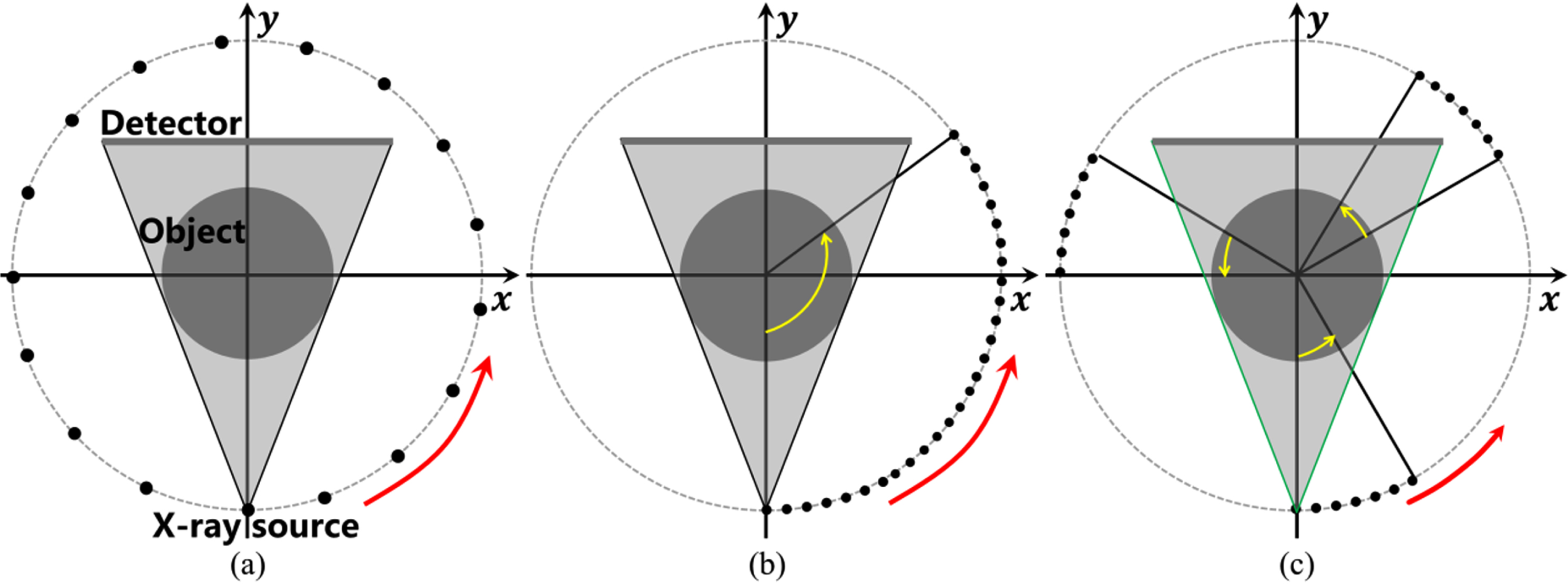
Typical CT sampling modes: (a) few-view sampling, (b) limited-angle sampling, (c) SLA sampling.

It is worth noting that when X-ray source and detector rotate at a high speed, turning on and off the tube voltage at low frequency will lead to segmental limited-angle (SLA) sampling, as shown in Fig. 1(c). In this mode, the X-ray source and detector still rotate around the object like few-view sampling mode. Turning on and off the tube voltage at low frequency means that when the tube voltage is turned on at a certain view angle, it is kept at a constant value for a time period before it is turned off. In another word, SLA sampling does not require rapid switching of the tube voltage. Repeat the above operation until the X-ray source rotate around the rotation center for one circle. Since SLA sampling involves several limited-angle samplings, it only needs to turn on and off the tube voltage a few times. When the voltage is off, CT system cannot collect projection data, so the acquired projection data is incomplete. Specifically, the projection view angles are divided into several clusters and distributed in the range of 360 degrees. The projection data under each cluster is limited-angle CT data. But SLA CT data is different from ordinary limited-angle CT data that are concentrated in a limited angular range. In some other applications, the acquired projection data show similar characteristics with SLA CT data. For example, in CT systems with multiple X-ray source/detector pairs, when each pair of X-ray source/detector rotates a small angular range, the collected projection data is aggregated into several beams and is incomplete [15, 16]. However, this configuration limits the size of the field of view, which is only used for interior tomography and it increases the economic cost. Besides, SLA sampling has been used in multienergy CT reconstruction [17, 18]. In this case, under each energy acquisition, the projection data is restricted in a limited angular range. To remove potential shading artifacts, the structural information of a prior image is incorporated into reconstruction model [19]. In this case, complete structural information of the object can be obtained, although it may be contaminated by motion artifacts or shading artifacts.

As far as we know, we cannot easily acquire the complete structural information of the object in SLA CT. In spite of that, compared to limited-angle CT reconstruction, SLA sampling actually reduces the difficulty of image reconstruction [8, 9]. However, the images reconstructed by simultaneous algebraic reconstruction technique (SART) still suffer from obvious artifacts. In this work, we aim to reduce the artifacts by exploring structural prior of CT images. Classical reconstruction method based on total variation (TV) assumes that the target image is piecewise constant, which has been used in some CT applications and shown good performance [20 –23]. However, it cannot effectively suppress shading artifacts in limited-angle CT [11, 24]. Since SLA sampling involves several limited-angle samples, the artifacts of SLA CT images like those of limited-angle CT images. As shown in Fig. 2, the artifacts change slowly like the shadow of the object, we call them shading artifacts for short. In fact, TV-based method used in SLA CT reconstruction can reduce the shading artifacts, but some residual artifacts remain [9]. In our previous work on SLA CT reconstruction, we define multi-direction total variation (MDTV) based on the direction information of the shading artifacts [9]. MDTV method can reduce artifacts, but CT image quality can be further improved. As we know, image gradient magnitude can be treated as adaptive weights to recover image structure. Following this idea, weighted anisotropic total variation (wATV) [25] is used for SLA CT reconstruction. Recently, methods based on image gradient L0 (GradL0) are proposed to reduce the shading artifacts [11 , 27]. Minimizing GradL0 does not penalize pixels with large gradient magnitude, but tends to penalize pixels with small gradient magnitude [28]. The shading artifacts change slowly, which often produce small gradient magnitudes. Therefore, minimizing GradL0 can suppress the shading artifacts, however, it seems not so effective to determine the importance of image structures [29], so some image structure may not be well recovered.

Fig. 2

In MLCT, intermittently reducing the number of segments can realize SLA sampling. This combination can reduce scanning time and reduce the load of X-ray tube and to improve the throughput of CT system.

In order to eliminate the potential disadvantages of the above reconstruction methods, a new reconstruction method is presented for SLA CT reconstruction. We incorporate image structure prior into reconstruction model to guide structure recovery and to reduce artifacts. In this work, we use relative total variation (RTV) [30] to regularize SLA CT reconstruction, and call it RTV method for short. RTV term has been widely applied to other reconstruction applications because of its capability of extracting image structures [19 , 31]. Different form the adaptive weights in wATV term, local statistics information of image gradients is used to refine structure prior so that RTV term meets our requirements for adaptive weights. The mentioned statistics information can be stated as follows, partial derivatives generated by structures often show the same direction, while those generated by noise often show different directions; besides, the pixel values of shading artifacts change slowly, while pixel values of image structures often change sharply. Based on this observation, RTV term can distinguish image structures from the shading artifacts. Then, we use a two-step algorithm to solve the RTV-regularized reconstruction model. Experimental results are reported to show the effectiveness of the presented method.

In the remainder of this article, we first introduce SLA sampling, related reconstruction methods, and present our method in Section II. We report simulation experiments and real CT data experiments in Section III. And finally, we conclude and report some discussions in Section IV.

2 Methodology

2.1 Brief introduction of SLA CT

In addition to reducing tube voltage or tube current, multiple ways can be used to reduce X-ray radiation dose, such as few-view sampling and limited-angle sampling. Few-view sampling requires frequently turning on and off the tube voltage, which demands for high technical requirements and hinders the wide application of this strategy [9]. Reducing X-ray pulse frequency can acquire few-view projection data, which, however, only acquire limited photon quantity in the environment of a rapidly rotating CT gantry. Limited-angle sampling is easy to realize, however, the reconstructed images often encounter obvious artifacts that are difficult to remove [10 , 24]. In addition, a multi-slit collimator can block some X-rays from passing through patients, which can be used in traditional CT based on circular scan trajectory [32] and spiral CT [33] to reduce radiation dose. However, motion patterns and positions of the multi-slit collimator need to be optimized carefully. And this strategy requires hardware modification to CT system. To the best of our knowledge, in medical CT, a practical under-sampling scheme has not been demonstrated in the challenging environment of a rapidly rotating CT gantry. In industrial CT, reducing X-ray radiation dose is not an urgent matter, but reducing scanning time or improving CT system throughput may be an important research topic. Reducing the turntable speed can be used to achieve few-view projection data, but it needs a long time. Thus, a practical under-sampling method is also necessary for industrial CT.

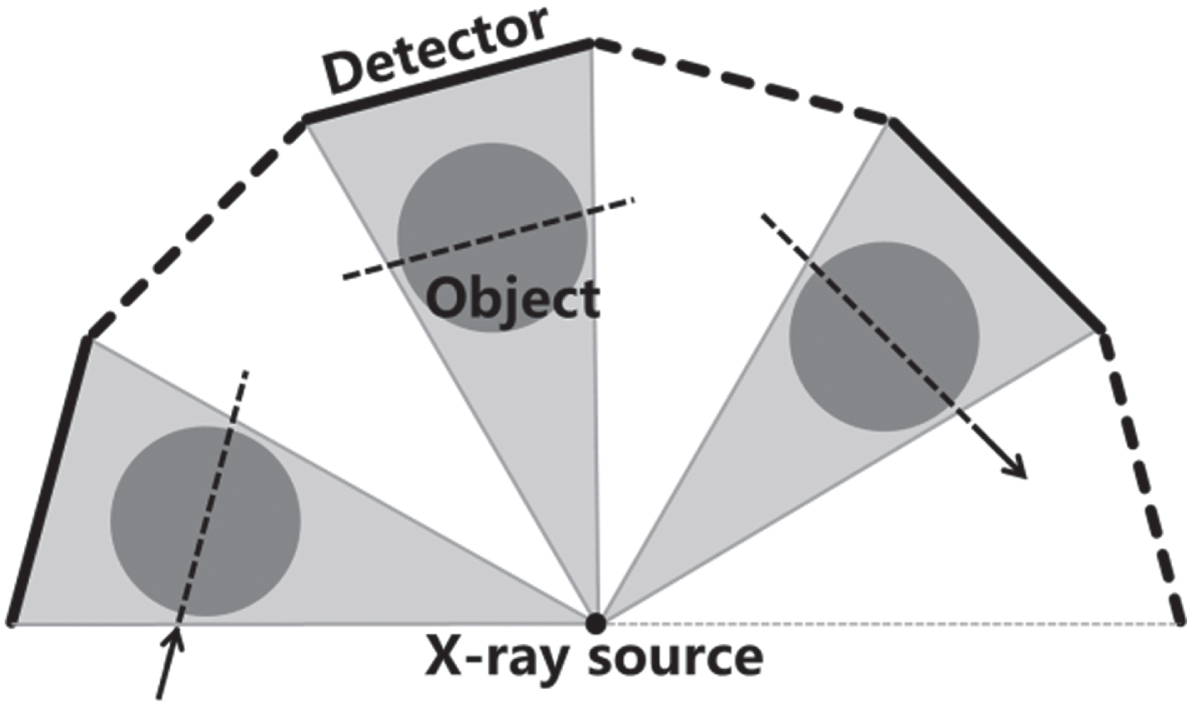
SLA sampling may be an appropriate choice, which can avoid rapid switching of tube voltage, and the acquired CT data has lower data correlation than limited-angle CT [9], so it is conducive to reconstructing high-quality images. Realizing SLA sampling only needs to turn on and off the tube voltage a few times in medical CT, which reduces technical difficulty. In industrial CT, multisegment straight-line CT (MLCT) [34 –37] scanning has been proposed to be a practical method. For example, in industrial online detection and safety inspection for baggage, MLCT may be a choice. Intermittently reducing the number of segments in MLCT can realize SLA sampling, as shown in Fig. 3. This combination reduces scanning time and the load of X-ray tube to improve the throughput of CT system. In a word, SLA sampling has the potential to be a practical under-sampling scheme in medical and industrial CT applications.

Fig. 3

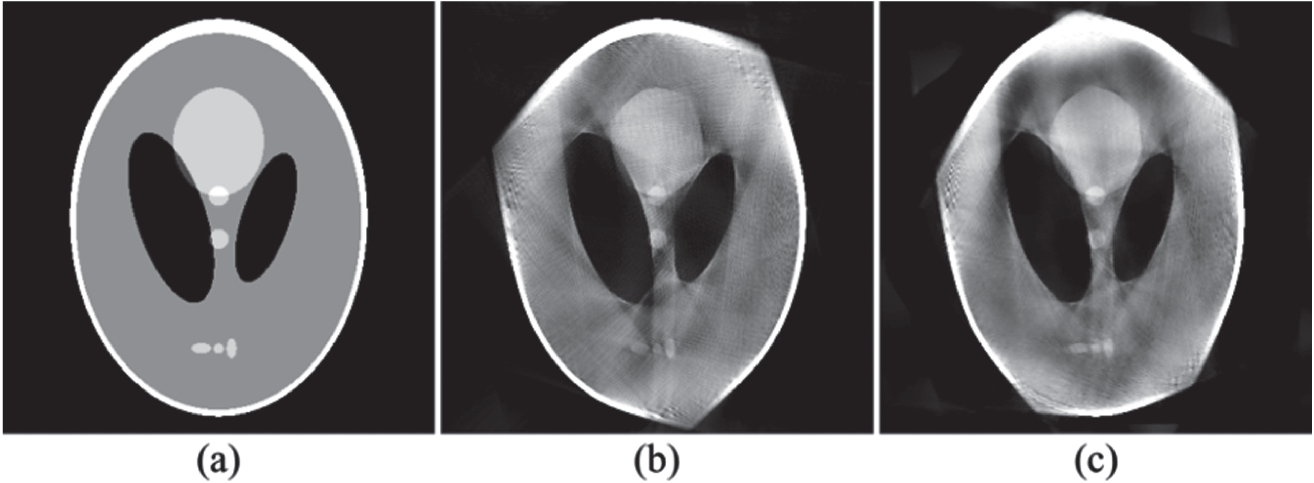
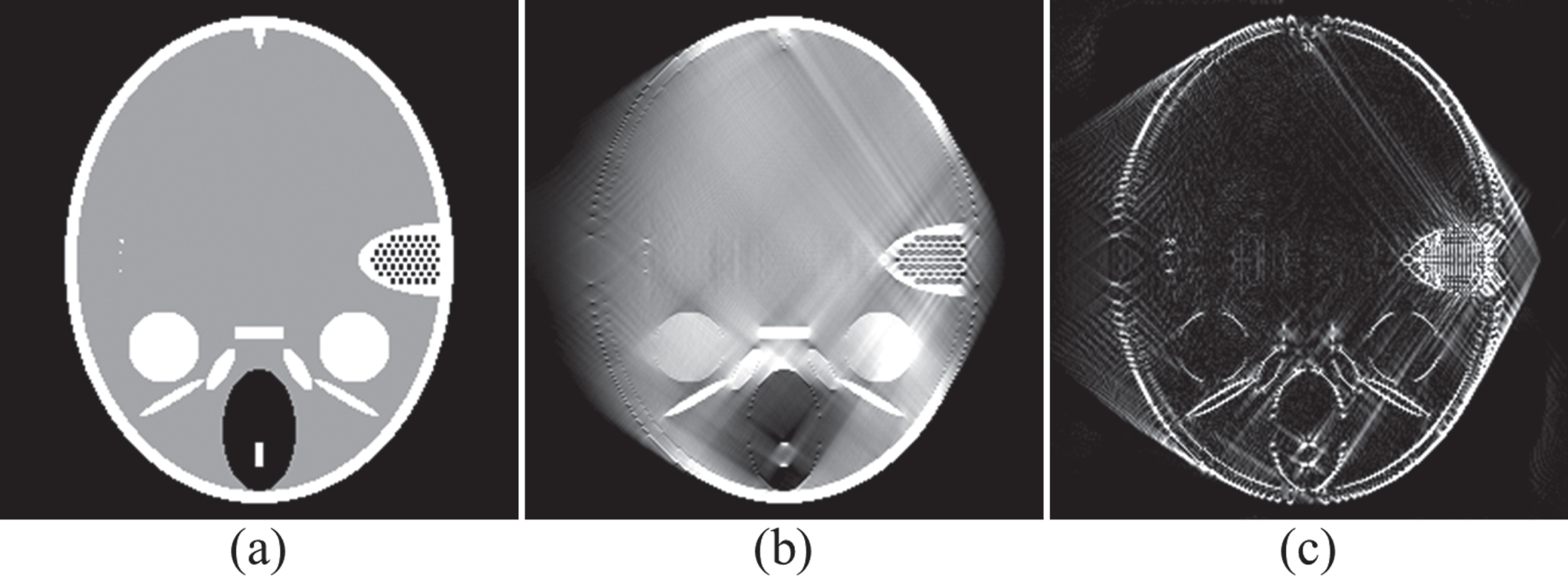
The shading artifacts distribution in SLA CT, (a) Shepp-Logan phantom, (b) image with shading artifacts distributed in 3 directions, (c) image with shading artifacts distributed in 5 directions.

2.2 MDTV-based reconstruction method

Total variation (TV) -based reconstruction model can be expressed as follows, $min_{f ⩾ 0} {∥ f ∥}_{TV}, s . t . Rf = p,$ (1) where matrix R with size of M × N is used for calculation of projection data p with size of M × 1. Term

_TV of image f with size of N × 1 is defined as the L1 norm of image gradient magnitude [21, 22], ${∥ f ∥}_{TV} = \sum_{n = 1}^{N} \sqrt{{(\partial_{x} f)}_{n}^{2} + {(\partial_{y} f)}_{n}^{2}}$ , where (∂_xf) _n and (∂_yf) _n are discrete differences (partial derivatives) at n^th pixel along x- and y- direction. Solving problem (1) means minimizing L1 norm of image gradient magnitude with constrains of projection data p. Image sparsity in the gradient domain is enhanced. Physically, all image gradient magnitudes contribute to TV norm, so solving problem (1) means equally penalizing or minimizing all image gradient magnitudes.

In our previous work on SLA CT reconstruction [9], we use directional total variation (DTV) to define MDTV as follows, ${∥ f ∥}_{MDTV} = \sum_{i = 1}^{N_{SLA}} {∥ f ∥}_{α, TV}$ (2) where N_SLA is the number of the segments in SLA sampling.

_α,TV is the DTV, it is defined as, ${∥ f ∥}_{α_{i} TV} = \sum_{n = 1}^{N} | D_{α_{i}} f_{n} |$ . As shown in Fig. 4, $| D_{α_{i}} f_{n} | = \frac{f_{α_{i}} - f_{n}}{δ_{α_{i}}}$ is the directional difference along the direction determined by the straight line with an included angle α_i (0 ⩽ α_i ⩽ π/4) with the positive direction of the x-axis. f_{α_i} is the interpolated pixel value and δ_{α_i} is the distance between n^th pixel and the interpolation point. Figure 4 shows the directional difference calculation in a special case of 0 ⩽ α_i ⩽ π/4, other cases can be found in Reference [9]. Generally, the direction of the angular bisector of each successive angular range is selected as one direction to calculate DTV. In SLA CT, the shading artifacts are distributed in multiple directions, as shown in Fig. 3. Based on this fact, MDTV enhances image sparsity in these directions to reduce shading artifacts. Nevertheless, the method based on MDTV may blur structure information. To solve MDTV reconstruction model, SART is first used to get an initial image, then the gradient descent algorithm is used to minimize MDTV. We call this method MDTV method for short.

Fig. 4

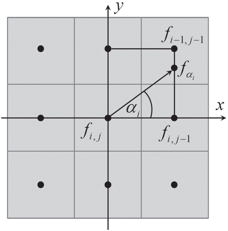
Diagram of the directional difference calculation (0 ⩽ α_i ⩽ π/ - 4).

2.3 wATV-based reconstruction method

In addition to structural information, one can use image gradient information to determine the penalty intensity for current gradient magnitude. Following this idea, weighted anisotropic total variation (wATV) is defined as follows, ${∥ f ∥}_{wATV} = \sum_{n = 1}^{N} \frac{\sqrt{{(\partial_{x} f)}_{n}^{2}}}{| {(\partial_{x} f)}_{n} | + τ} + \frac{\sqrt{{(\partial_{y} f)}_{n}^{2}}}{| {(\partial_{y} f)}_{n} | + τ} .$ (3)

It should be noted that weights 1/(|∂_xf) _n| + τ and 1/(| (∂_yf) _n| + τ) vary with pixel positions, where τ is a small constant. When the weights are generated by potential prior or reference image, that is to say, they are fixed, wATV becomes traditional weighted anisotropic total variation [25, 38]. In this work, we still call this term in (4) wATV term for convenience. The adaptive weights reduce the dependence of wATV on gradient magnitudes, so it is closer to L0 norm than TV norm [29]. Physically, wATV based method is to minimize weighted gradient magnitudes. Minimizing wATV tends to reconstruct piecewise constant images. In SLA CT, gradient magnitudes generated by artifacts or noise are often small, that is, | (∂_xf) _n| and | (∂_yf) _n| are small, so their reciprocals 1/(| (∂_xf) _n| + τ) and 1/(| (∂_yf) _n| + τ) are large. Image structures often mean sharp changes in pixel values, that is, gradient magnitudes are often large, so their weights are small. Minimizing wATV is propitious to suppressing artifacts and noise and retaining structure information. To solve reconstruction model regularized by wATV, we pre-compute the adaptive weights using reconstructed image at previous step, and then minimize wATV using gradient descent algorithm. For short, we call this method wATV method.

2.4 GradL0-regularized reconstruction method

Image gradient L0 (GradL0) is defined as follows [28], ${∥ f ∥}_{GradL 0} = \sum_{n = 1}^{N} # {| {(\partial_{x} f)}_{n} | + | {(\partial_{y} f)}_{n} | \neq 0} .$ (4) where #{ | (∂_xf) _n| + (∂_yf) _n ≠ 0 } outputs 1 when | (∂_xf) _n| + | (∂_yf) _n| ≠ 0 holds. GradL0 measure is not a norm mathematically since

c · f

_GradL0 ≠ c ·

_GraL0, which is often used to measure image sparsity. GradL0 term does not rely on gradient magnitude information, so minimizing GradL0 does not penalize pixels with large gradient magnitude but tends to penalize pixels with small gradient magnitude. The shading artifacts often produce small gradient magnitudes, so they are expected to be suppressed by GradL0 minimization. In order to solve GradL0-regularized reconstruction model, we refer the algorithm used in Ref. [11]. For short, we call it GradL0 method.

2.5 Proposed reconstruction method

In SLA CT reconstruction, we endeavor to reduce artifacts and preserve image structures. Following the strategy used in wATV, we must be concerned with that whether the weights are reliable due to the negative impact of artifacts and noise. In order to release the impact, we use relative total variation (RTV) to extract reliable structure prior. RTV of image f is defined as follows [30], $RTV (f_{n}) = \frac{\sum_{m \in w (n)} h_{n, m} \cdot | (\partial_{x} f)_{m} |}{| \sum_{m \in w (n)} h_{n, m} \cdot (\partial_{x} f)_{m} | + ɛ} + \frac{\sum_{m \in w (n)} h_{n, m} \cdot | (\partial_{y} f)_{m} |}{| \sum_{m \in w (n)} h_{n, m} \cdot (\partial_{y} f)_{m} | + ɛ} .$ (5) where the two numerators are called windowed total variation (WTV), which is denoted by T_x (f_n) and T_y (f_n). The two denominators are called windowed inherent variation (WIV), which is denoted by I_x (f_n) and I_y (f_n). So $RTV (f_{n}) = \frac{T_{x} (f_{n})}{I_{x} (f_{n}) + ɛ} + \frac{T_{y} (f_{n})}{I_{y} (f_{n}) + ɛ}$ . w (n) is the window used to calculate WTV and WIV, and is centered around n^th pixel, h_n,m is a weighting function and takes the form, h_m,n ∝ exp(- ((x_m - x_n) ² + (y_m - y_n) ²)/ - (2σ²)), parameter σ is the standard deviation, and parameter ɛ a small constant. When window w (n) shrinks to one pixel, RTV term degenerates to $\frac{| (\partial_{x} f)_{n} |}{| (\partial_{x} f)_{n} | + ɛ} + \frac{| (\partial_{y} f)_{n} |}{| (\partial_{y} f)_{n} | + ɛ}$ and it is equivalent to wATV. So RTV term can be viewed as a generalization of wATV. However, different from wATV, the partial derivatives in w (n) are used to calculate WIV and weight WTV. When calculating WIV, we first calculate the weighted summation of all partial derivatives in w (n) using h_n,m. Then we obtain its absolute value. When calculating WTV, we first obtain the absolute values of all partial derivatives in w (n), then use weighting function to calculate their weighted summation.

TV is defined as the L₁ norm of the image gradient. All noise, artifact, and structure pixels increase TV value, which show that the TV responds to the pixel value changes. The numerator term in equation (5) can be viewed as weighted TV because of weighting function h_m,n. According to its definition, we know WTV is also responsive to the pixel value changes. Both WTV and WIV are calculated via absolute value operation and weighted summation operation but calculated in reverse order. A key observation is that partial derivatives generated by structures often show the same direction, while those generated by noise often show different directions. Therefore, a local window that contains more noise will generate a small WIV, since opposite partial derivatives in the same window cancel out each other. A local window that contains more structures will generate a larger WIV. We here use a noisy CT image Fig. (5a) of the FORBILD head phantom to show how to obtain the structure information. First, partial derivative image along the x-direction is calculated and shown in Fig. 5(b). Partial derivatives in flat regions are noisy and they often have small amplitudes. In order to see their behavior clearly, image profiles indicated by the solid line are shown in Fig. 5(e). Then weighting function h_n,m is used to calculate the filtered version of the partial derivative image. The filtered image is shown in Fig. 5(c). Finally, we acquire the WIV values of image f, as shown in Fig. 5(d). The weights induced by WIV help to identify image structures and get rid of the impact of noise.

Fig. 5

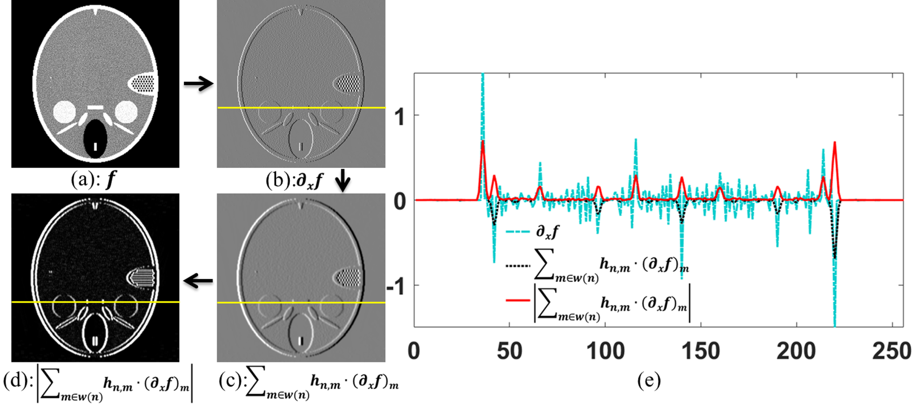
Calculating WIV values of image f: (a) A noisy CT image of FORBILD head phantom, (b) partial derivative image, (c) filtered version of (b), (d) WIV image, (e) image profiles marked by the solid lines in the left panel. The acquired values along the solid line highlight image structures and get rid of the impact of noise.

Next, on question is that can WIV distinguish image structures from shading artifacts? We know that the pixel values in the region of shading artifacts change slowly, while image structures often mean sharp changes in pixel value. WIV is defined as the absolute value of the weighted summation of all partial derivatives in a local window. Therefore, as shown in Fig. 6, a local window that contains more shading artifacts will generate a small WIV, since shading artifacts produce small partial derivatives. A local window that contains more structures will generate a larger WIV. Hence, WIV can also distinguish image structures from shading artifacts. RTV-based reconstruction model can be expressed as follows, $min_{f ⩾ 0} | | Rf - p | |_{2}^{2} + γ \cdot \sum_{n = 1}^{N} RTV (f_{n}) .$ (6)

Fig. 6

(a) FORBIL head phantom, (b) image with shading artifacts, (c) WIV image of image (b). Pixel values in the region of shading artifacts change slowly, so a local window that contains shading artifacts will generate a small WIV. The weight induced by WIV can effectively identify image structures.

The first term uses SLA CT data to reconstruct an initial guess of CT image. The second term uses two observations above to reduce shading artifacts and recover structures. Where f denotes represents the image to be reconstructed, and f_n represents the n^th pixel value of image f. For short, we call this method RTV method.

The proposed reconstruction model (6) is nonconvex, so we endeavor to find a reasonable solution that may be a local minimizer. In this work, we use a simple two-step algorithm to solve problem (6). Minimizing the first term is a quadratic optimization problem, whose solution can be acquired by f^k+1/2 = (R^TR) ^-1R^Tp. However, computing the inverse matrix (R^TR) ^-1 is hard because of large size of R. In this work, we linearize the first term at f^(k), and acquired the following equation, $| | Rf - p | |_{2}^{2} = | | {Rf}^{(k)} - p | |_{2}^{2} + 〈 R^{T} ({Rf}^{(k)} - p), f - f^{(k)} 〉 + γ_{1} \cdot | | f - f^{(k)} | |_{2}^{2} .$ (7)

Then, solving problem (6) is transferred to solving the following problem, $min_{f ⩾ 0} 〈 R^{T} ({Rf}^{(k)} - p), f - f^{(k)} 〉 + γ_{1} \cdot | | f - f^{(k)} | |_{2}^{2} + γ \cdot \sum_{n = 1}^{N} RTV (f_{n}) .$

Note, this problem can be reformulated as follows, $min_{f ⩾ 0} 〈 (1 / - γ_{1}) \cdot R^{T} ({Rf}^{(k)} - p), f - f^{(k)} 〉 + | | f - f^{(k)} | |_{2}^{2} + (γ / - γ_{1}) \cdot \sum_{n = 1}^{N} RTV (f_{n})$

Immediately, we can get the following equivalent expression via adding a constant term, $| | (1 / - 2 γ_{1}) \cdot R^{T} ({Rf}^{(k)} - p) | |_{2}^{2}$ , $min_{f ⩾ 0} | | f - (f^{(k)} - (1 / - 2 γ_{1}) \cdot R^{T} ({Rf}^{(k)} - p)) | |_{2}^{2} + (γ / - γ_{1}) \cdot \sum_{n = 1}^{N} RTV (f_{n}) .$ (8)

Therefore, we can solve problem (6) via the following two steps,

Subproblem-1: $f^{(k + 1 / - 2)} = f^{(k)} - (1 / - 2 γ_{1}) \cdot R^{T} ({Rf}^{(k)} - p),$ (9)

Subproblem-2: $f^{(k + 1)} = \underset{f ⩾ 0}{arg min} | | f - f^{(k + 1 / - 2)} | |_{2}^{2} + η \cdot \sum_{n = 1}^{N} RTV (f_{n}) .$ (10) where f^(k) denotes an intermediate image at k^th iteration, which is used as the input image of subproblem-1. And f^(k+1/-2) denotes the output result of subproblem-1, γ₁ and η = γ/ - γ₁ are two parameters. Subproblem-1 uses SLA CT data and image at previous step to acquire an initial guess f^(k+1/-2), which is closer to our expected solution than f^(k). In order to deal with Subproblem-1, we must know the system matrix R. Because it is a huge matrix, we use SART to deal with the storage problem of system matrix. In short, in order to avoid inverse operation, we choose linearization. In order to deal with the storage problem of system matrix, we finally chose to use SART to solve Subproblem-1.

Subproblem-2 uses RTV regularization to reduce shading artifacts. Parameter η affects the effect of RTV regularization. A large value may smooth structural information, while a small value can retain more details but may not reduce shading artifacts and noise. A proper parameter η is expected to render visually decent image f^(k+1), which is used as the input image of subproblem-1 at next iteration and is closer to our expected solution. Subproblem-2 can be solved by the algorithm designed in Ref. [30]. For easy reading, we briefly describe this algorithm here. First, x- and y-direction parts of RTV are respectively decomposed and re-arranged into a quadratic term and a non-linear term as follows (x-direction part), $\begin{matrix} \sum_{n} \frac{\sum_{m \in w (n)} h_{n, m} \cdot | (\partial_{x} f)_{m} |}{| \sum_{m \in w (n)} h_{n, m} \cdot (\partial_{x} f)_{m} | + ɛ} = \sum_{n} \frac{\sum_{m \in w (n)} h_{n, m} \cdot | (\partial_{x} f)_{m} |}{I_{x} (f_{n}) + ɛ} \\ = \underset{N iterms}{\underset{︸}{\sum_{m \in w (1)} \frac{h_{1, m}}{I_{x} (f_{1}) + ɛ} \cdot | (\partial_{x} f)_{m} | + \sum_{m \in w (2)} \frac{h_{2, m}}{I_{x} (f_{2}) + ɛ} \cdot | (\partial_{x} f)_{m} | + \dots \sum_{m \in w (N)} \frac{h_{N, m}}{I_{x} (f_{N}) + ɛ} \cdot | (\partial_{x} f)_{m} |}} \\ = \sum_{m} \sum_{n \in w (m)} \frac{h_{n, m}}{I_{x} (f_{n}) + ɛ} | (\partial_{x} f)_{m} | \approx \sum_{m} \sum_{n \in w (m)} \frac{h_{n, m}}{I_{x} (f_{n}) + ɛ} \frac{1}{| (\partial_{x} f)_{m} | + τ} (\partial_{x} f)_{m}^{2} \\ = \sum_{m} u_{x, m} v_{x, m} (\partial_{x} f)_{m}^{2} . \end{matrix}$ (11) where I_x (f_n) denotes |∑_m∈w(n)h_n,m · (∂_xf) _m|, that is WIV. And parameter τ is used for numerical stability. We can see that u_x,mv_x,m is the non-linear term and $(\partial_{x} f)_{m}^{2}$ is the quadratic term, and we have the following equations, $u_{x, m} = \sum_{n \in w (m)} \frac{h_{n, m}}{I_{x} (f_{n}) + ɛ}, v_{x, m} = \frac{1}{| (\partial_{x} f)_{m} | + τ} .$ (12)

Then, for y-direction part of RTV, we have the following equations, $u_{y, m} = \sum_{n \in w (m)} \frac{h_{n, m}}{I_{y} (f_{n}) + ɛ}, v_{y, m} = \frac{1}{| (\partial_{y} f)_{m} | + τ} .$ (13)

Based on these operations, subproblem-2 can be transformed into solving the following problem, $\underset{φ_{f}}{arg min} (φ_{f} - φ_{f^{(k + 1 / - 2)}})^{T} (v_{f} - v_{f^{(k + 1 / - 2)}}) + γ_{1} \cdot (φ_{f}^{T} C_{x}^{T} U_{x} V_{x} C_{x} φ_{f} + φ_{f}^{T} C_{y}^{T} U_{y} V_{y} C_{y} φ_{f}) .$ (14) where image f and f^(k+1/-2) are rewritten in matrix form φ_f and φ_{f
^(k+1/-2)}, respectively. C_x and C_x are two Toeplitz matrices. U_x, U_y, V_x, and V_x are four diagonal matrices and the diagonal elements are u _x,m, u _y,m, v_x,m, and v _y,m, respectively. Then, an effective algorithm is designed to find a numerically stable solution. First, in order to solve problem (14), U_x, U_y, V_x, and V_x are calculated from current reconstruction result using equation (12) and (13). Second, minimizing the objective function of problem (14) is transformed into solving the following linear system, $[E + γ_{1} (C_{x}^{T} U_{x}^{(t)} V_{x}^{(t)} C_{x} + C_{y}^{T} U_{y}^{(t)} V_{y}^{(t)} C_{y})] \cdot φ_{f}^{(t)} = φ_{f^{(k + 1 / - 2)}}^{(t)} .$ (15) where E denotes an identity matrix. Equation (15) shows the linear equation solved in t-step. In this step, we denote the number of iterations by N_RTV. The coefficient matrix in the front of function $φ_{f}^{(t)}$ is a sparse positive definite Laplace matrix.

In order to solve problem (8), we first use SART to decrease the energy of the data fidelity item. Then, RTV of the intermediate image is minimized by solving problem (10) and it has been proved that the used algorithm can quickly converge to a solution. Its solution can be viewed as a proximal map of image f^(k+1/-2). Overall, a complete main cycle of our algorithm is a composition of a gradient descent step and a proximal map. We can conclude that the final solution f^* is a fixed point of the proximal operator. Since the reconstruction model (6) is nonconvex, we can only find a local minimizer.

To sum up, we list the whole algorithm flow in Table 1. Parameter N_out is the maximum iteration steps of the algorithm. Parameter ξ₁ measure the relative error between images at two adjacent steps. If parameter ξ₁ < ξ₀, the algorithm will terminate in advance.

Table 1

Algorithm flow of RTV method for SLA CT reconstruction

Algorithm 1: SLA CT reconstruction
1: initialization: input p, η, ɛ, τ, σ, ξ₀, N_RTV, N_out
2: for i = 1:N_out, do
3: execute SART step to deal with Equation (9);
4: calculate u_x,m, u_y,m, v_x,m, and v_y,m using Equations (12 and 13);
5: solve problem (15) iteratively;
6: output image f⁽ⁱ⁺¹⁾ and compute ξ₁ = \|\|f⁽ⁱ⁺¹⁾ - f⁽ⁱ⁾\|\|/\|\|f⁽ⁱ⁺¹⁾\|\|
7: if ξ₁ < ξ₀, exit;
8: end for 9: output: the reconstructed image.

2.6 Parameter selection

In RTV method, some parameters need to be determined: η, ɛ, τ, σ, N_RTV, ξ₀ and N_out. Parameter N_out is the total number of iterations, which is set to 2000 in this work. When ξ₁ is less than 10^–6 (ξ₀), the algorithm will terminate. Then we also give reference values for other parameters. In addition, in order to more clearly show the impact of parameters on image quality, we assign different values to one parameter, and then plot the RMSE and SSIM of their respective reconstructed images in Fig. 7. From the first-row image in Fig. 7, we can see that a proper parameter η is conductive to reconstructing higher-quality image, it varies in the range of [0.001, 0.005] for all experiments on digital phantom. For real data experiments, it should be adjusted cautiously and mainly varies in the range of [0.000001, 0.00003]. N_RTV is the number of iterations to solve Subproblem-2, and the second-row images in Fig. 7 show that parameter N_RTV larger than or equal to 4 is desirable for obtaining high-quality images, and it is set to 6 for all experiments in this work. Parameters ɛ is used to avoid zero denominators and varies in [0.00001, 0.01]. A small ɛ is our regular choice. Parameters τ is also used to avoid zero denominators and varies in [0.00001, 0.001] in this work. Finally, we can see that parameter σ has little impact on the image quality. We analyze the reason is that it is vital for structure extraction from texture; however, the used phantom has no texture information and obvious noise. It varies in the range of [1, 3] in this paper to save computing resource. According to the trend of these curves, we can determine appropriate reconstruction parameters in numerical simulation experiment. In real CT applications, only limited-angle CT data is available, there is no reference image or the reference image is difficult to obtain. The selection of regularization parameter depends too much on the experience and manual selection may lead to unrealistic reconstructions. Thus, real CT reconstruction calls for methods that adaptively determine regularization parameters. And that’s going to be one of the main topics in our next study.

Fig. 7

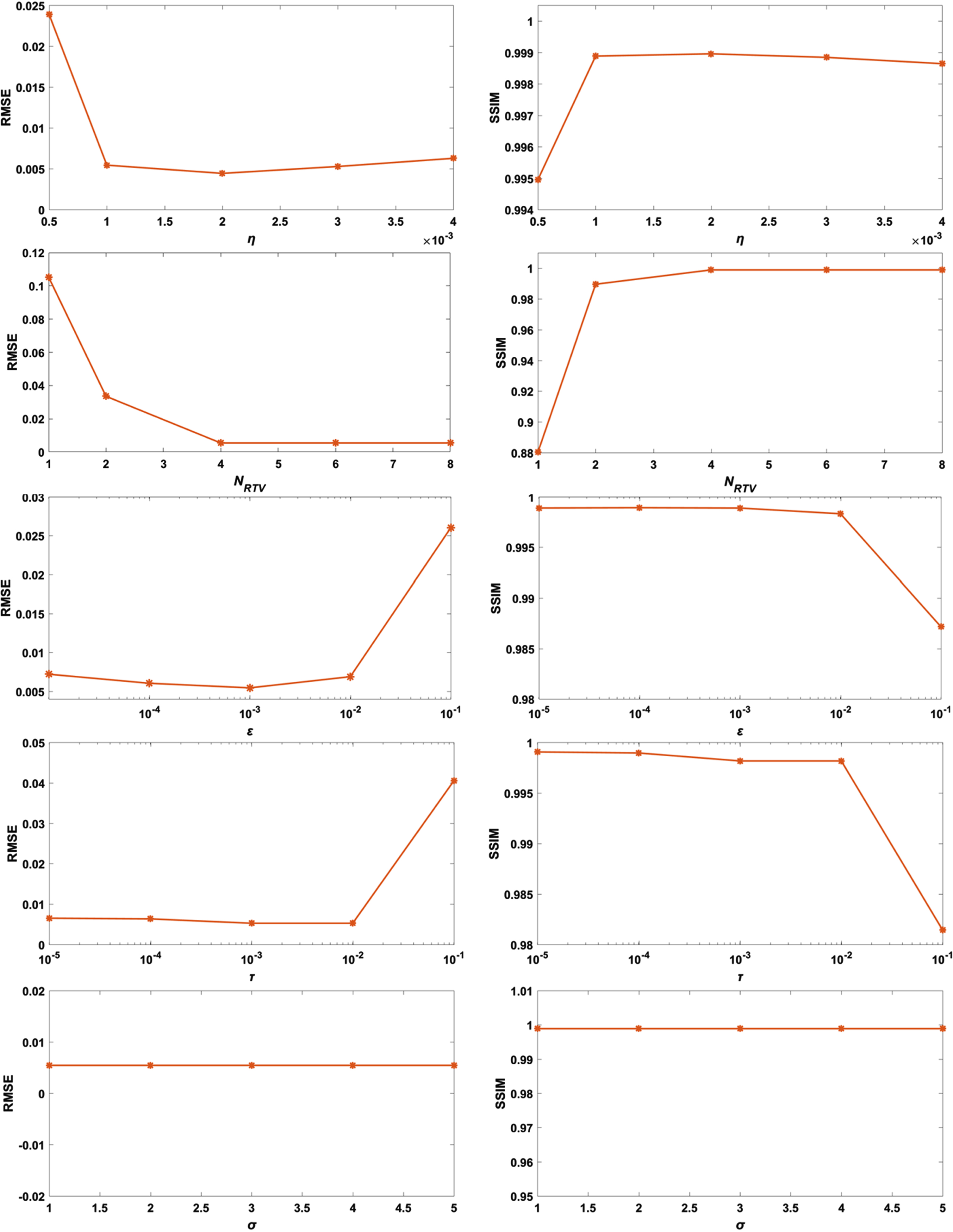
Impact of reconstruction parameters on image quality.

3 Numerical and experimental studies

In this section, experiments on digital phantoms and real CT data are reported to prove the effectiveness of the proposed reconstruction method. First, we use two digital phantoms (Fig. 8) to evaluate the performance of different methods. The results of reconstructed images and their quantitative evaluation will be displayed. Second, real CT data experiments are used to verify the effect of our method in real scenes. All the experiments are run on a laptop computer (8.0 GB memory, 2.40 GHz CPU, NVIDIA GeForce GTX 1650 card, Windows 10 64-bit system environment).

Fig. 8

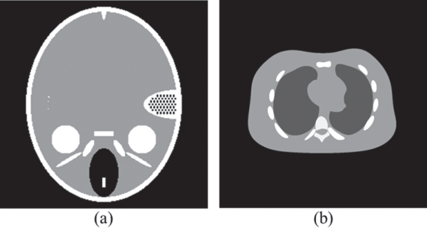
(a) Reference image of FORBILD head phantom, (b) Reference image of NCAT phantom.

3.1 Verification of the proposed reconstruction method

We first use the FORBILD head phantom and NCAT phantom to verify the proposed reconstruction method. We use these experiments to show that the effectiveness of our method is due to its ability to distinguish image structures from shading artifacts and noise. The two phantoms consist of 256×256 pixels. The geometric parameters used for scanning and CT reconstruction are listed in Table 2. Poisson noise and Gaussian noise are added to noise-free projection data. The incident photon number is 1×10⁵. The mean value and variance of Gaussian noise is 0 and 0.1% ×||p||_∞, respectively. In this work, RTV method is compared to MDTV, wATV, and ADM-L0 methods. In addition to reconstructed images, their root mean square error (RMSE), peak signal to noise ratio (PSNR), and structural similarity (SSIM) [39] are calculated for image quality comparison.

Table 2
Scanning and reconstruction parameters in simulation experiments

Parameter Values

Focus-to-object distance (mm) 500

Focus-to-detector distance (mm) 800

Detector Size 512

Length of detector (mm) 512

Reconstructed image size 256×256

Scanning angular interval (degree) 1

Parameter	Values
Focus-to-object distance (mm)	500
Focus-to-detector distance (mm)	800
Detector Size	512
Length of detector (mm)	512
Reconstructed image size	256×256
Scanning angular interval (degree)	1

3.1.1 Experiments on FORBILD head phantom

In this section, the projection data in the range of [(0°, 30°] ∪ [120°, 150°] ∪ [240°, 270°] is used for image reconstruction. MDTV, wATV, ADM-L0 and RTV method are used to reconstruct CT image, their results are shown in the first row of Fig. 9, and their residual images are shown in the second row. In this experiment, reconstruction parameters for all methods are shown in Table 3. We can observe that ADM-L0 and our method can recover sharp image structures and reduce more artifacts than MDTV and wATV methods. When compare ADM-L0 and our method, it is difficult to see some differences from the reconstructed images, but we can observe their different performance from the residual images. The FORBILD head phantom is piecewise constant, and the residual image of ADM-L0 method is piecewise constant, but some image edges are not well recovered. Despite all this, their image quality approaches to each other closely. To show the superiority of RTV method, their RMSE, PSNR, and SSIM are calculated and listed in Table 4, which indicate the CT image obtained by the proposed method is closer to the reference image.

Fig. 9

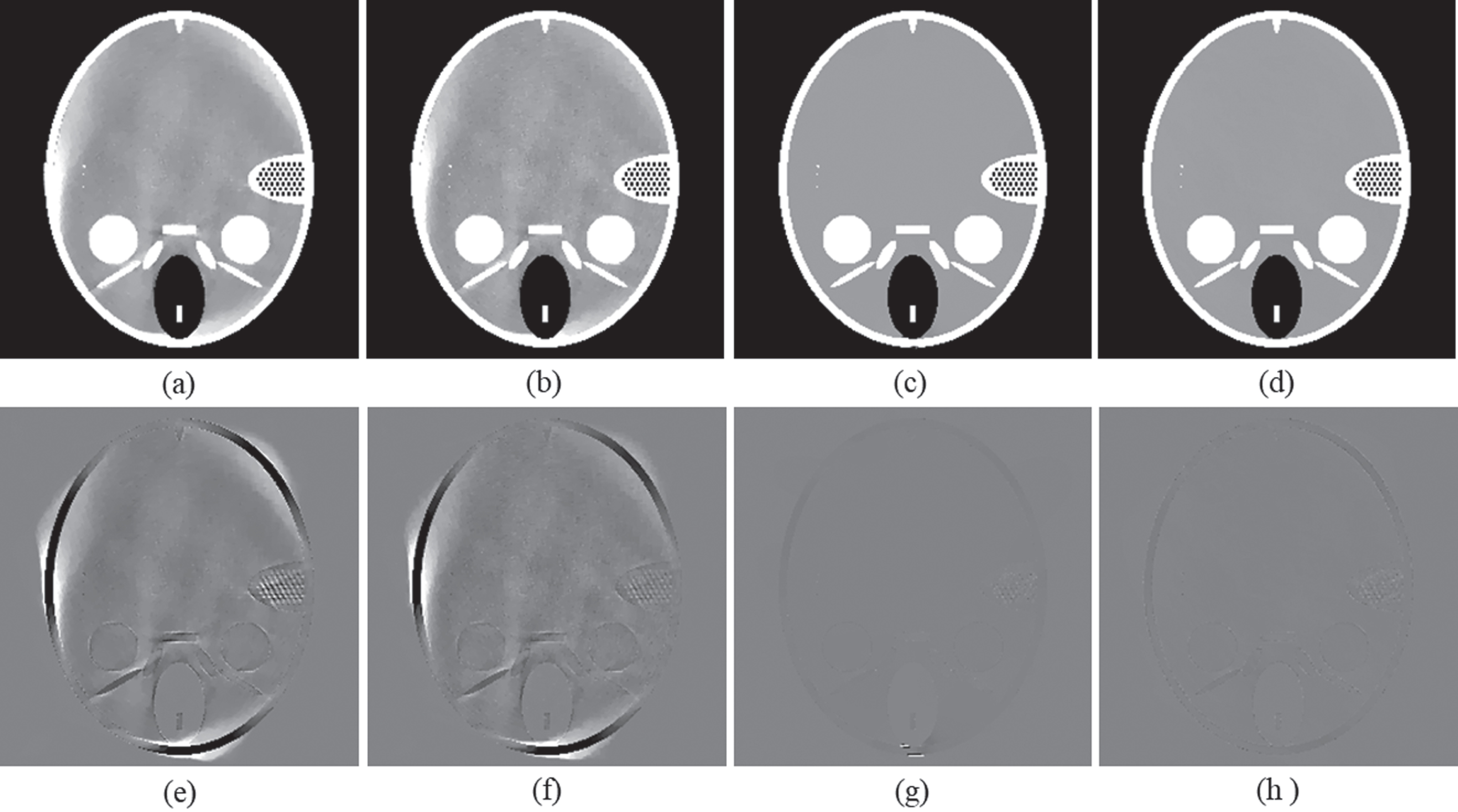
Images of the FORBIL head phantom reconstructed from projection data in the range of [0°, 30°] ∪ [120°, 150°] ∪ [240°, 270°], (a) MDTV, (b) wATV, (c) ADM-L0, (d) RTV method; (e), (f), (g), and (h) are their residual images. The display window for CT images is [0.8, 1.2] and for residual images [–0.2, 0.2].

Table 3

Reconstruction parameters for the FORBILD head phantom and the reconstructed images are shown in Fig. 9

MDTV	wATV	ADM-L0	RTV
$\begin{matrix} α = 0.1, \\ K = 20 \end{matrix}$	$\begin{matrix} α = 0.1, \\ K = 20 \end{matrix}$	$\begin{matrix} λ = 0.004, \\ κ = 2 \\ μ = 0.2 \end{matrix}$	$\begin{matrix} η = 0.001, \\ σ = 2, ɛ = τ = 0.001, \\ N_{RTV} = 6 \end{matrix}$

Table 4

SSIM, RMSE and PSNR of CT images of FORBILD head phantom, and the reconstructed images are shown in Fig. 9

	MDTV	wATV	ADM-L0	RTV
SSIM	0.9633	0.9724	0.9765	0.9989
RMSE	0.0652	0.0488	0.0134	0.0038
PSNR	28.83	31.34	42.56	53.50

In addition to this experiment, the projection data in the range of [0°, 18°] ∪ [72°, 90°] ∪ [144°, 162°] ∪ [216°, 234°] ∪ [288°, 306°] is used for image reconstruction. All competing methods are used to reconstruct CT image. Reconstructions results are shown in the first row of Fig. 10, and their residual images are shown in the second row. Reconstruction parameters for all methods are the same as that shown in Table 3. We can see that obvious artifacts appear in the images reconstructed by TVM and wATV methods, while ADM-L0 and RTV method can reduce more shading artifacts. RMSE, PSNR, and SSIM of these CT images are calculated and listed in Table 5, which indicate the CT image obtained by RTV method is closer to the reference image.

Fig. 10

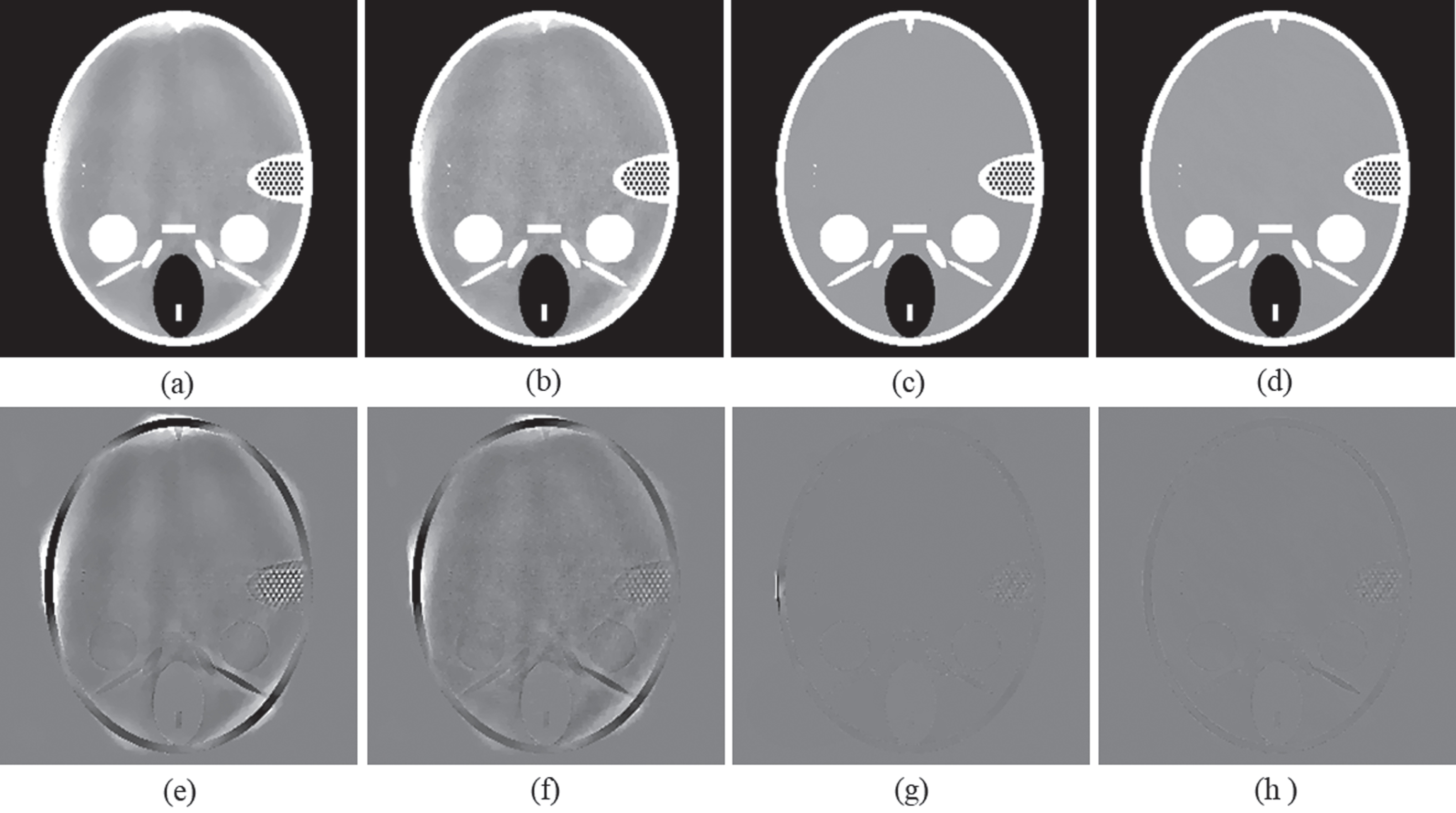
Images of the FORBILD head phantom reconstructed from projection data in the range of [0°, 18°] ∪ [72°, 90°] ∪ [144°, 162°] ∪ [216°, 234°] ∪ [288°, 306°], (a) MDTV, (b) wATV, (c) ADM-L0, (d) RTV; (e), (f), (g), and (h) are their residual images. The display window for CT images is [0.8, 1.2] and residual images [–0.2, 0.2].

Table 5

SSIM, RMSE and PSNR of CT images of FORBILD head phantom, and the reconstructed images are shown in Fig. 10

	MDTV	wATV	ADM-L0	RTV
SSIM	0.9712	0.9788	0.9862	0.9988
RMSE	0.0550	0.0389	0.0155	0.0040
PSNR	30.30	33.32	41.30	53.14

In order to clearly show the superiority of our method, we plot profiles of the images in the first experiment on FORBILD head phantom along some row, the figures are shown in Fig. 11(a) and (b). And Fig. 11(b)is the close-up of the selected region in (a). We can see that the profile of our method is closer to the reference image.

Fig. 11

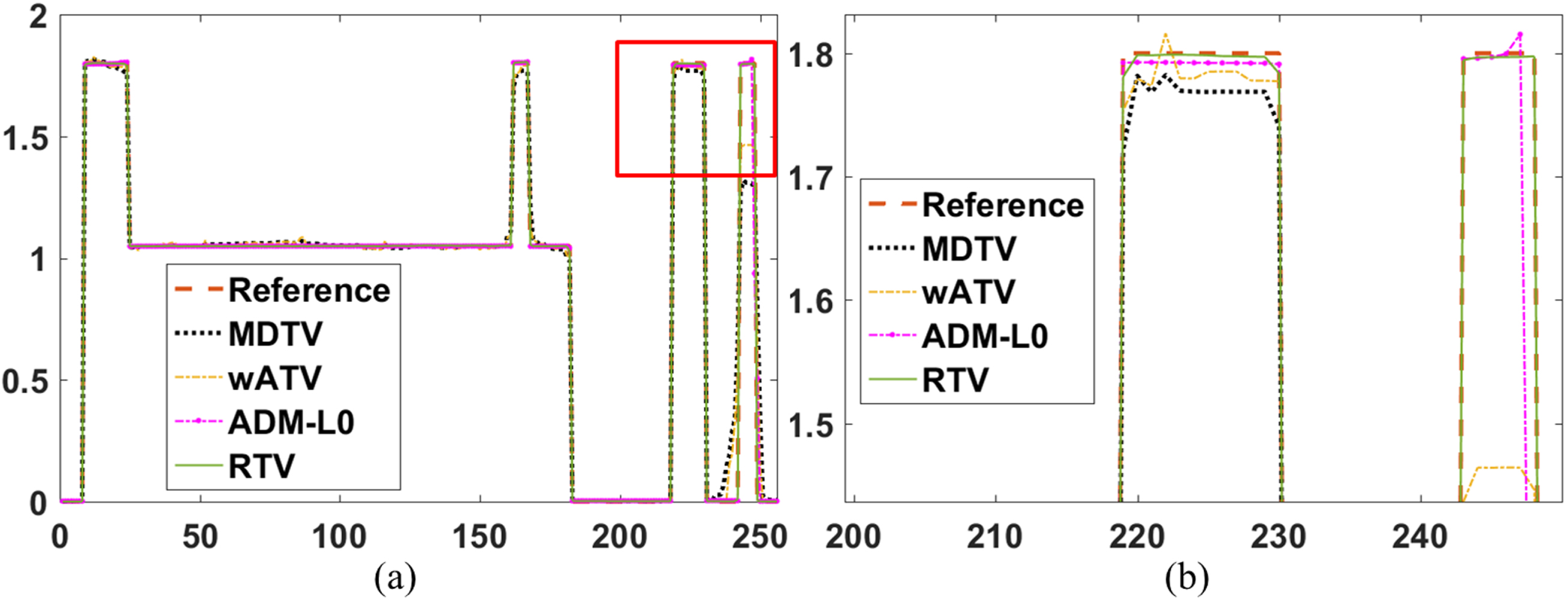
Image profiles in the first experiment on FORBILD head phantom: (a) horizontal profiles along middle image row. (b) is the close-up of the local regions in (a).

SLA sampling can be combined with multisegment straight-line CT (MLCT) scanning. Intermittently reducing the number of segments in MLCT can realize SLA sampling, this under-sampling strategy is conducive to improve the throughput of industrial CT system. Besides, the source fan-beam coverage in MLCT is often less than 180 degrees. In the new experiment, we assume that the projection data is in the range of [0°, 30°] ∪ [60°, 90°] ∪ [120°, 150°]. Then, all methods are used for image reconstruction. Main reconstruction parameters are adjusted referring to those in Table 3. The reconstructed images are not shown in this paper for short. Their RMSE, PSNR, and SSIM of these images are calculated and listed in Table 6, which show that RTV method performs best.

Table 6

SSIM, RMSE and PSNR of CT images of FORBILD head phantom, and the images are reconstructed from projections in the range of [0°, 30°] ∪ [60°, 90°] ∪ [120°, 150°]

	MDTV	wATV	ADM-L0	RTV
SSIM	0.9787	0.9799	0.9804	0.9989
RMSE	0.0504	0.0419	0.0173	0.0037
PSNR	31.06	32.67	40.32	53.82

3.1.2 Experiments on NCAT phantom

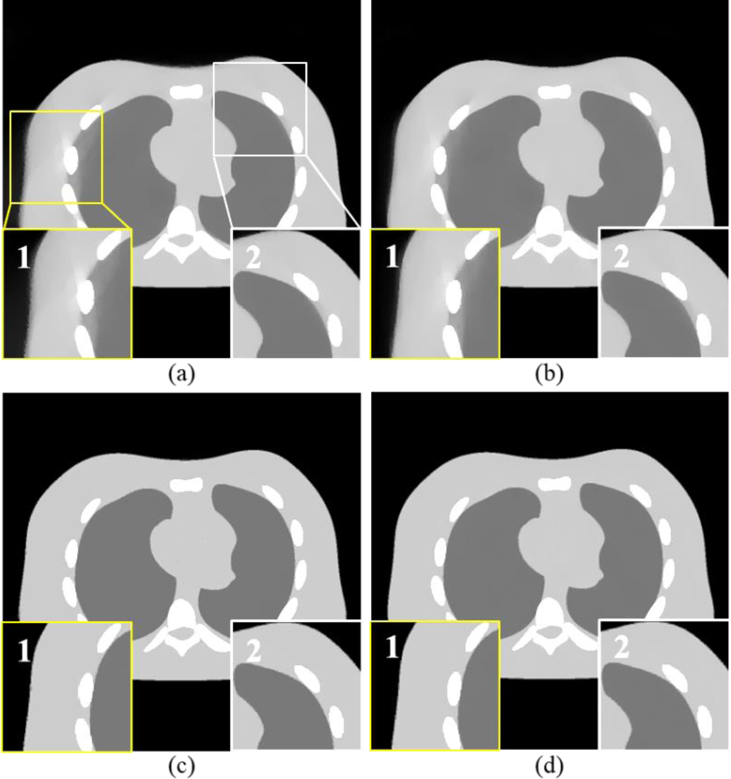
In this section, NCAT phantom is used to compare different reconstruction methods. The projection data in the range of [0°, 30°] ∪ [120°, 150°] ∪ [240°, 270°] is first used for image reconstruction. The reconstructed images are shown in Fig. 12. The reconstruction parameters are shown in Table 7. Thanks to the advantages of SLA sampling, the images reconstructed by all methods have little difference. In order to clearly show their differences, we select two local regions and display their close-ups. Images reconstructed by MDTV and wATV suffer from shading artifacts, which can be observed in their close-ups. ADM-L0 removes most of the shading artifacts, so no obvious artifacts remain in the image or its close-ups. However, ADM-L0 cannot completely recover some image structures (close-up 1). The image reconstructed by our method is closer to the reference image. There is no obvious artifact in its close-ups and image structures are recovered well. Their RMSE, PSNR, and SSIM are listed Table 8, which show that our method performs best, which coincides with the results obtained from image comparison.

Fig. 12

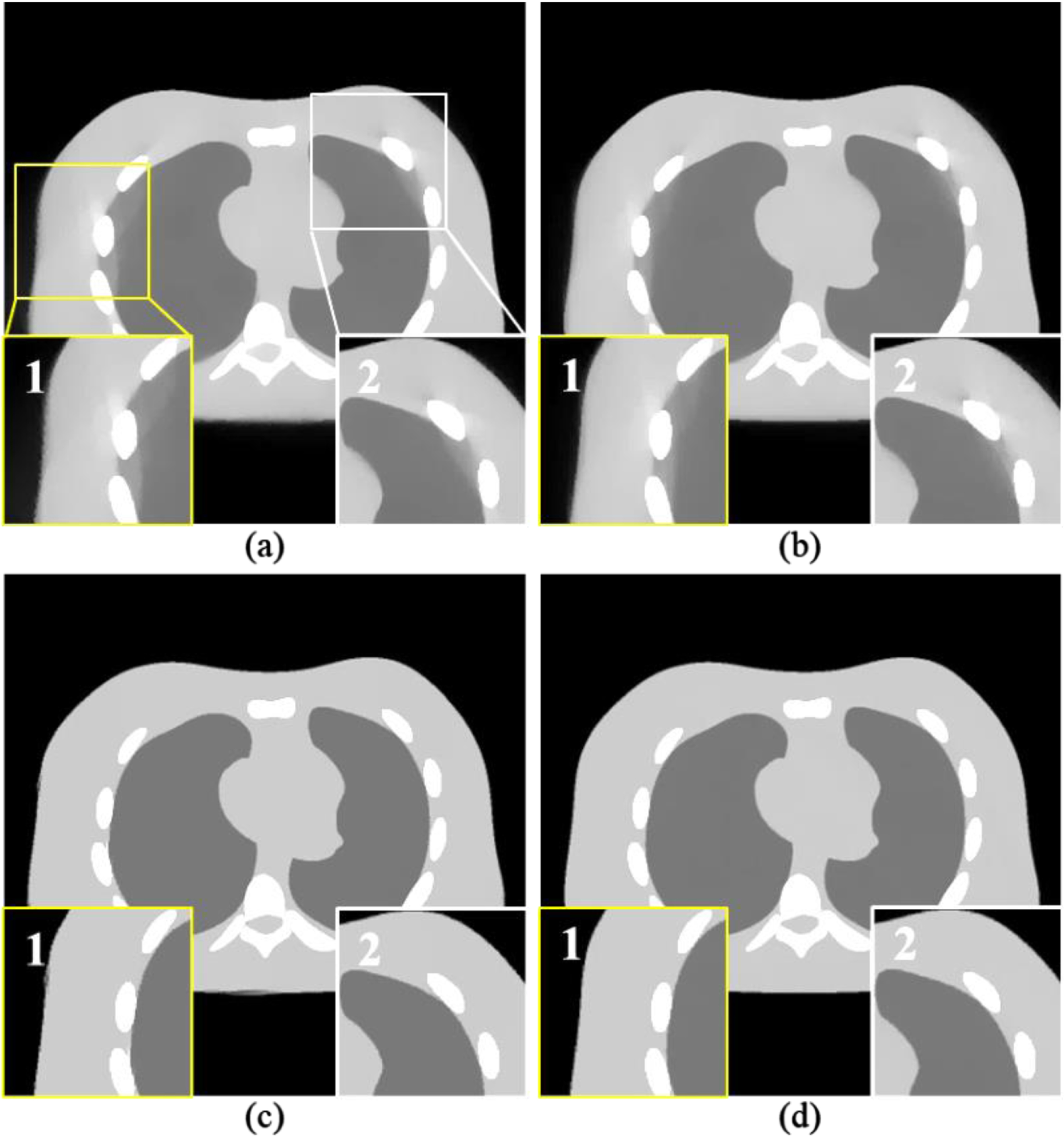
Images of the NCAT phantom reconstructed from projection data in the range of [0°, 30°] ∪ [120°, 150°] ∪ [240°, 270°]. (a) MDTV, (b) wATV, (c) ADM-L0, (d) RTV method. Two local regions are selected for image quality comparison. The display window is [0, 3].

Table 7

Reconstruction parameters for the NCAT phantom and the reconstructed images are shown in Fig. 12

MDTV	wATV	ADM-L0	RTV
$\begin{matrix} α = 0.4, \\ K = 30 \end{matrix}$	$\begin{matrix} α = 0.4, \\ K = 20 \end{matrix}$	$\begin{matrix} λ = 0.02, \\ κ = 2 \\ μ = 0.2 \end{matrix}$	$\begin{matrix} η = 0.002, \\ σ = 2, ɛ = τ = 0.001, \\ N_{RTV} = 6 \end{matrix}$

Table 8

SSIM, RMSE and PSNR of CT images of the NCAT phantom, and the reconstructed images are shown in Fig. 12

	MDTV	wATV	ADM-L0	RTV
SSIM	0.9431	0.9652	0.9654	0.9961
RMSE	0.1037	0.0758	0.0422	0.0169
PSNR	31.73	34.45	39.54	47.49

When SLA sampling is combined with MLCT, the projection data of NCAT phantom in the range of [0°, 30°] ∪ [60°, 90°] ∪ [120°, 150°] is used for CT reconstruction. All methods are used for image reconstruction. Reconstruction results are shown in Fig. 13. Main reconstruction parameters are listed in Table 9. Like the results of previous experiment, MDTV and wATV cannot effectively remove the shading artifacts, which can be observed in their close-ups. ADM-L0 and our method reconstruct high-quality images. There are no obvious artifacts in their images or close-ups and image structures are recovered well. In order to compare them, RMSE, PSNR, and SSIM of these images are calculated and listed in Table 10. The image reconstructed by our method is closer to the reference image. Besides, we also plot image profile in the first experiment on the NCAT phantom, and the figures are shown in Fig. 14. Horizontal profiles are plotted as shown in Fig. 14(a). And Fig. 14(b) is the close-ups of the selected region in (a). We can see that the profile of our method is closer to the reference one.

Fig.13

Images of the NCAT phantom reconstructed from projection data in the range of [0°, 30°] ∪ [60°, 90°] ∪ [120°, 150°]. (a) MDTV, (b) wATV, (c) ADM-L0, (d) RTV method. Two local regions are selected for image quality comparison. The display window is [0, 3].

Table 9

Reconstruction parameters for the NCAT phantom and the reconstructed images are shown in Fig. 13

MDTV	wATV	ADM-L0	RTV
$\begin{matrix} α = 0.3, \\ K = 20 \end{matrix}$	$\begin{matrix} α = 0.4, \\ K = 20 \end{matrix}$	$\begin{matrix} λ = 0.02, \\ κ = 5 \\ μ = 0.2 \end{matrix}$	$\begin{matrix} η = 0.002, \\ σ = 2, ɛ = τ = 0.001, \\ N_{RTV} = 6 \end{matrix}$

Table 10

SSIM, RMSE and PSNR of CT images of the NCAT phantom, and the reconstructed images are shown in Fig. 13

	MDTV	wATV	ADM-L0	RTV
SSIM	0.9669	0.9763	0.9735	0.9973
RMSE	0.0812	0.0651	0.0246	0.0166
PSNR	33.85	35.76	44.22	47.63

Fig. 14

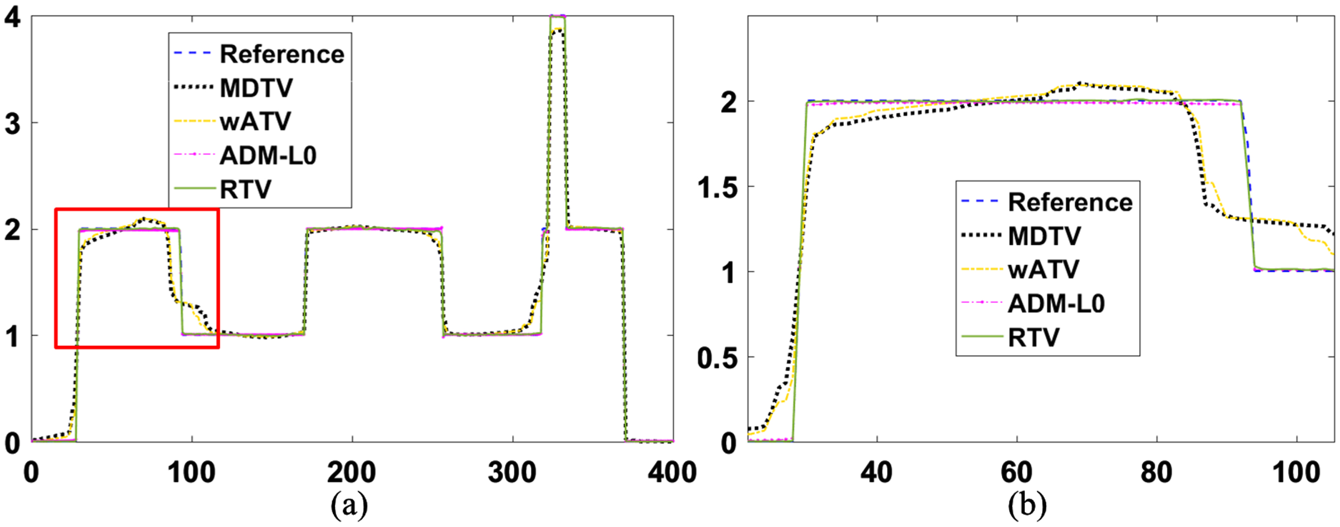
Image profiles in the first experiment on the NCAT phantom, (a) is horizontal profiles along certain image row. (b) is the close-up of the local regions in (a).

3.2 Convergence of RTV method

We take the previous experiment on the FORBILD head phantom as an example to study whether the presented algorithm can converge. The projection data is in the range of [0°, 30°] ∪ [120°, 150°] ∪ [240°, 270°]. The adopted algorithm in this work is to minimize the objective function in problem (6). Thus, the energy functional is first calculated to see whether it decreases during iteration process. Then, RMSE is plotted here to see if the intermediate image gradually approaches to the reference image. In order to calculate the energy functional, the data fidelity term and the regularization term are calculated. Data fidelity term $| | Rf - p | |_{2}^{2}$ is L2 norm of the projection data difference, which can be easily computed. Then we move our eyes to the calculation of the RTV term that is clearly defined as shown in Equation (5). Calculating RTV (f_n) mainly involves difference operations and convolution operations, where parameters σ, γ, and ɛ are the same as those in Table 3. Finally, energy curve and RMSE curve are plotted in Fig. 15, which has two y-axes. The left y-axis characterizes the value of objective function, and the right y-axis characterizes RMSE of output image at each iteration step. In this experiment, our algorithm terminates at iteration 1200, so the scale range of x-axis is 1 to 1200. Figure 15 shows that both two curves gradually descend to small and stable values. The descending energy curve shows that the used algorithm indeed optimizes the objective function in problem (6). The descending RMSE curve shows that this method can find a local minimizer close to real solution.

Fig. 15

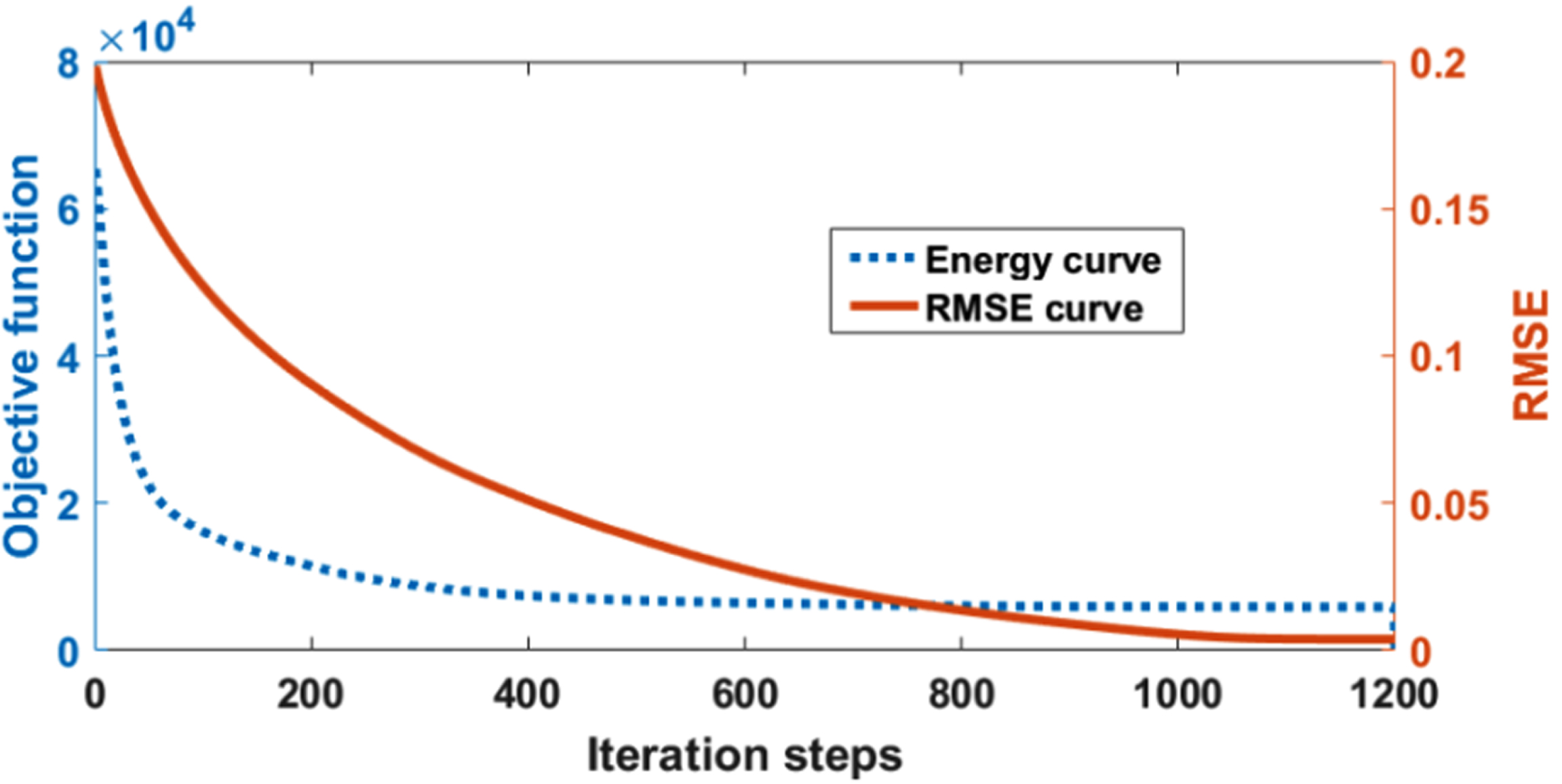
Energy curve and RMSE curve in experiment on the FORBILD head phantom. This figure has two y-axes, the left and right characterize the value of objective function and RMSE of reconstructed images, respectively. These two curves gradually descend to a small value.

3.3 Experiments on real CT data

Experiments on digital phantom show that the proposed method performs better than other competing methods in term of artifact reduction and structure preservation. In real CT applications, noise and potential artifacts may abate the performance of reconstruction methods. It is necessary to test all reconstruction methods in a more realistic situation. In this section, real CT data of a carved cheese [40] engraved with “CT” is used for image reconstruction. In order compare image quality, a reference image is reconstructed by SART (20 iterations) algorithm using complete projection data and the reference image is shown in Fig. 16(a).

Fig. 16

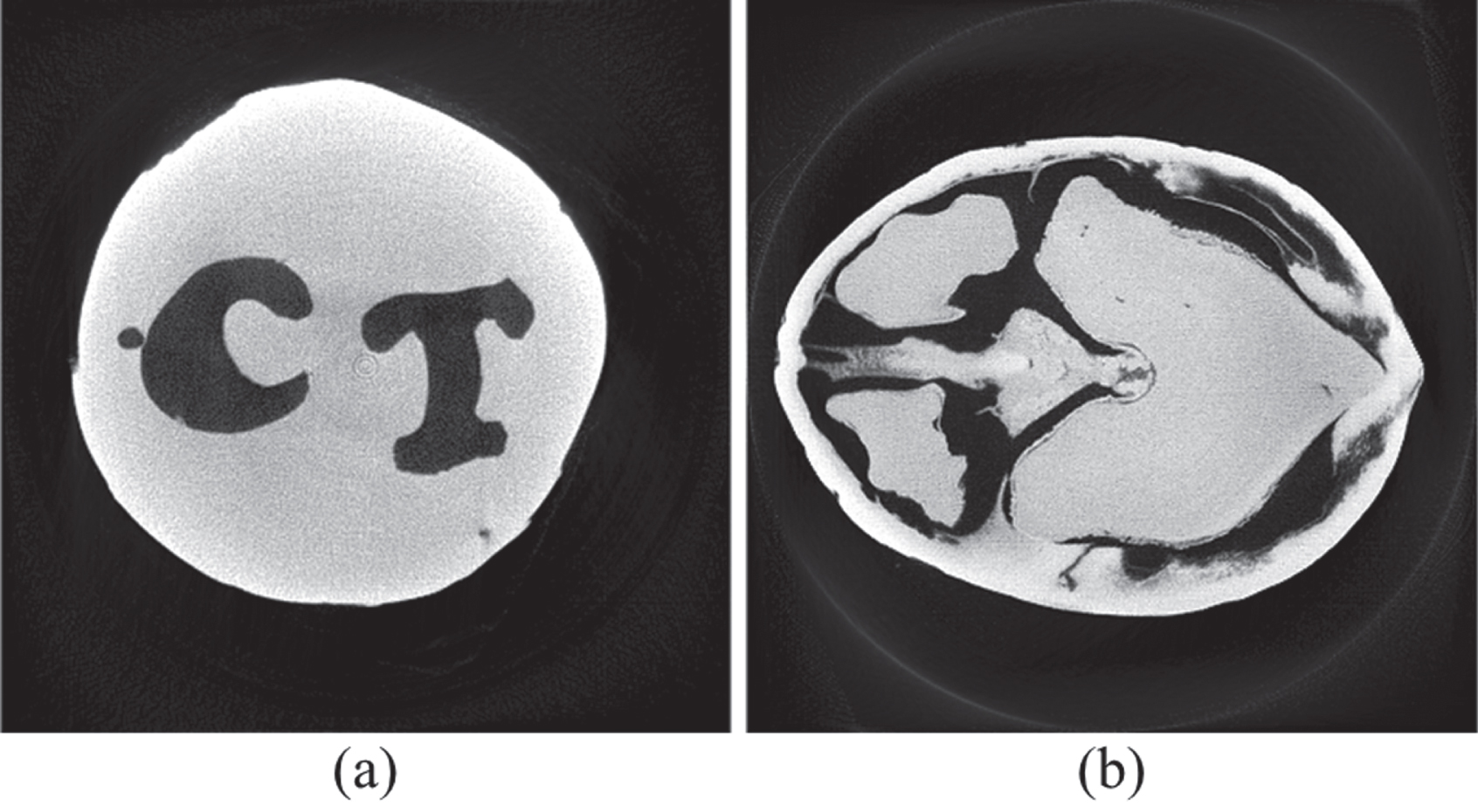
CT images of a carved cheese and a walnut, (a) carved cheese CT image, (b) walnut CT image. The display window is [0.01, 0.05] and [0 0.04], respectively.

First, the projections in the range of [0°, 30°] ∪ [120°, 150°] ∪ [240°, 270°] is used for image reconstruction. Reconstruction parameters are listed in Table 11. The reconstructed images are shown in Fig. 17. Images acquired by MDTV and wATV methods suffer from obvious blocky artifacts. ADM-L0 method can remove blocky artifacts; however, noise cannot be suppressed well, which can be observed in Fig. 17(c). Our method avoids obvious blocky artifacts and noise. Besides, their residual images are listed Fig. 18 to see differences between different methods. The residual images of MDTV and wATV methods encounter more shading artifacts, which can be observed in close-up 1 and 2 in Fig. 18(a) and (b). ADM-L0 method can suppress the shading artifacts, but it does not perform well in image edge preservation. As indicated by the arrows in close-up 2, our method can better recover some image structures than ADM-L0. And its residual image encounters the least artifacts.

Table 11

Reconstruction parameters for experiments on a carved cheese, whose CT images are shown in Fig. 17

MDTV	wATV	ADM-L0	RTV
$\begin{matrix} α = 0.3, \\ K = 20 \end{matrix}$	$\begin{matrix} α = 0.3, \\ K = 20 \end{matrix}$	$\begin{matrix} λ = 0.00005, \\ κ = 5 \\ μ = 0.2 \end{matrix}$	$\begin{matrix} η = 0.000004, \\ σ = 2, ɛ = 0.00001, \\ τ = 0.001, N_{RTV} = 6 \end{matrix}$

Fig. 17

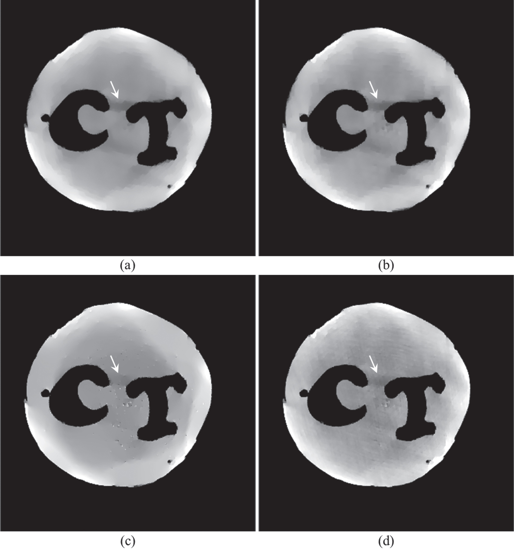
CT images of a carved cheese reconstructed from projection data in the range of [0°, 30°] ∪ [120°, 150°] ∪ [240°, 270°]. (a) MDTV, (b) wATV, (c) ADM-L0, (d) RTV method. The display window is [0.02, 0.05].

Fig. 18

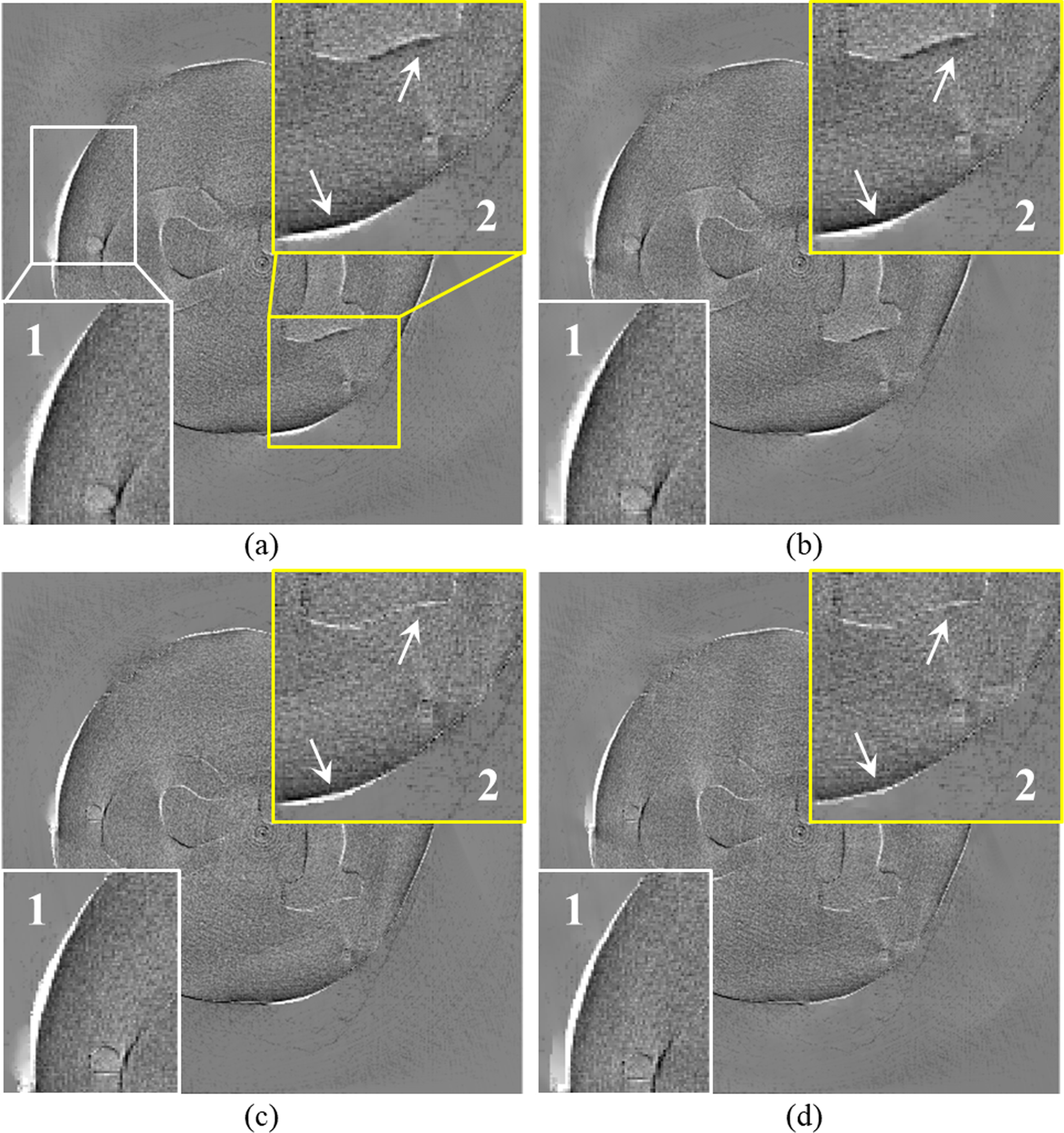
Residual images of different methods related to CT images shown in Figure 17: (a) MDTV, (b) wATV, (c) ADM-L0, (d) RTV method. The display window is [–0.02, 0.02].

When the projection data is in [0°, 30°] ∪ [60°, 90°] ∪ [120°, 150°], the reconstructed images are shown in Fig. 19. Reconstruction parameters are the same as those in Table 11. We can get results similar with the previous experiment. Images reconstructed by MDTV and wATV methods suffer from obvious artifacts, while ADM-L0 method and RTV method can remove blocky artifacts. When comparing ADM-L0 and RTV method, we can see ADM-L0 cannot suppress noise well, while our method avoids obvious noise. Their residual images are listed Fig. 20, which show that MDTV and wATV methods encounter more shading artifacts, which are indicated in close-up 1 (left local region) and 2 (right local region). ADM-L0 and our method can reduce some shading artifacts, but ADM-L0 does not perform well in image edge preservation as indicated by the arrows in close-up 2 in Fig. 20(c). From a comprehensively perspective, our method performs better in artifact reduction and structure preservation.

Fig.19

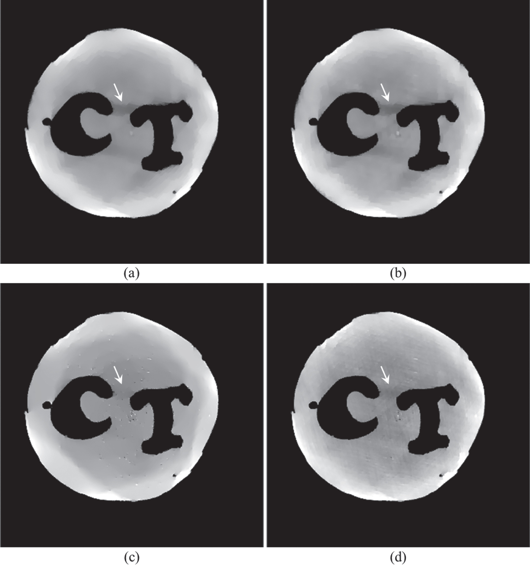
CT images of a carved cheese reconstructed from projection data in the range of [0°, 30°] ∪ [60°, 90°] ∪ [120°, 150°], (a) MDTV, (b) wATV, (c) ADM-L0, (d) RTV method. The display window is [0.02, 0.05].

Fig. 20

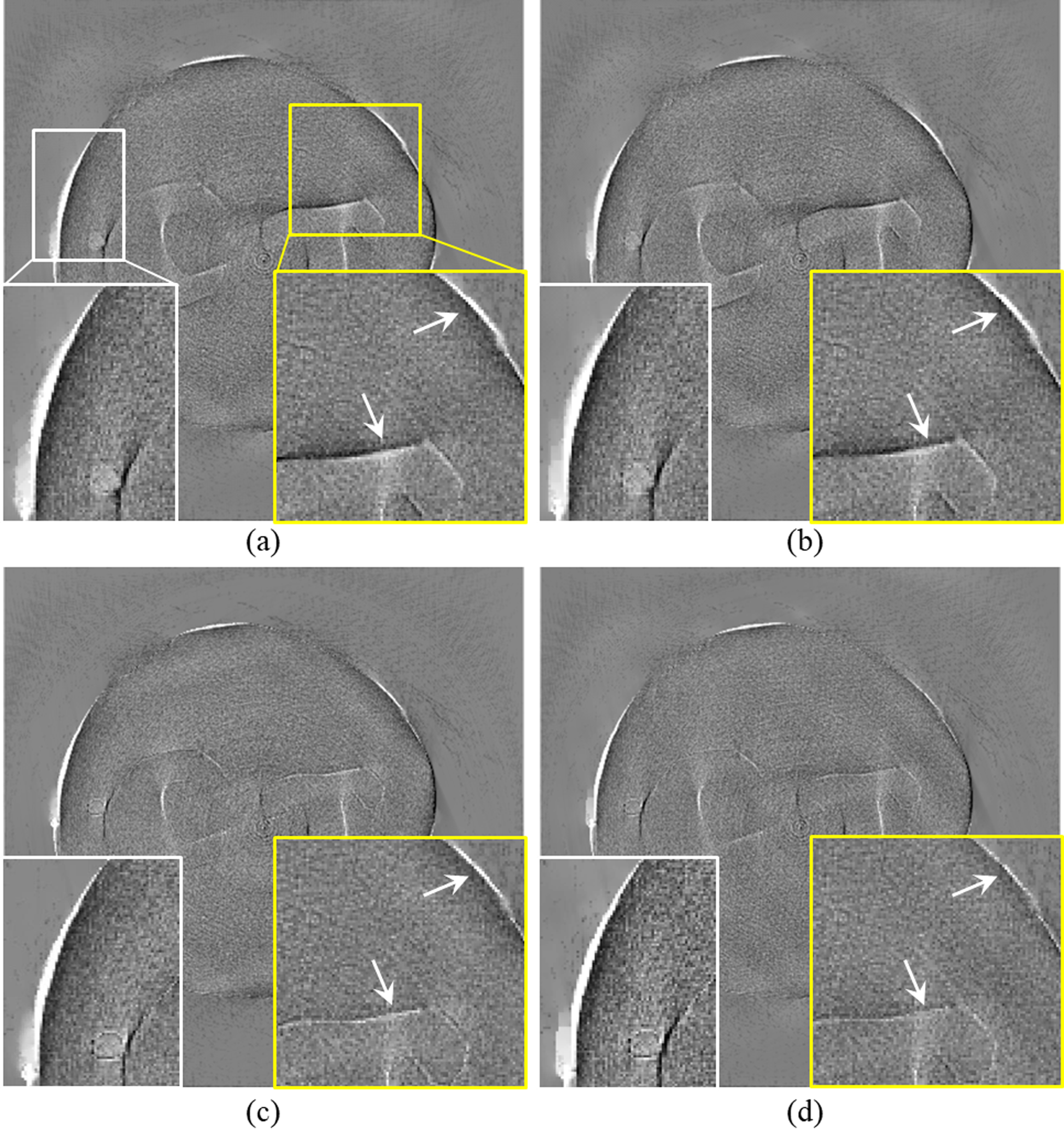
Residual images of different methods related to CT images shown in Figure 19: (a) MDTV, (b) wATV, (c) ADM-L0, (d) RTV method. The display window is [–0.02, 0.02].

In addition, real CT data of a walnut is used for image reconstruction since it has more details. A reference image is reconstructed by SART (20 iterations) using complete projection data and is shown in Fig. 16(b). Then the projection data in the range of [0°, 30°] ∪ [120°, 150°] ∪ [240°, 270°] is used for image reconstruction. The reconstructed images are shown in Fig. 21. We can see that images acquired by MDTV and wATV methods suffer from obvious shading artifacts. ADM-L0 method can remove some artifacts; however, noise cannot be suppressed well. Our method avoids obvious artifacts and noise. Besides, their residual images are listed Fig. 22. Clearly, the residual images of MDTV and wATV methods encounter more residual artifacts, which can be observed in close-up 1 in Fig. 22(a) and (b). ADM-L0 method can suppress the shading artifacts, but it does not perform well in image edge preservation, as indicated by the arrows in close-up 2. Our method can better recover some image structures than ADM-L0, and the residual image of our method encounters the least shading artifacts.

Fig. 21

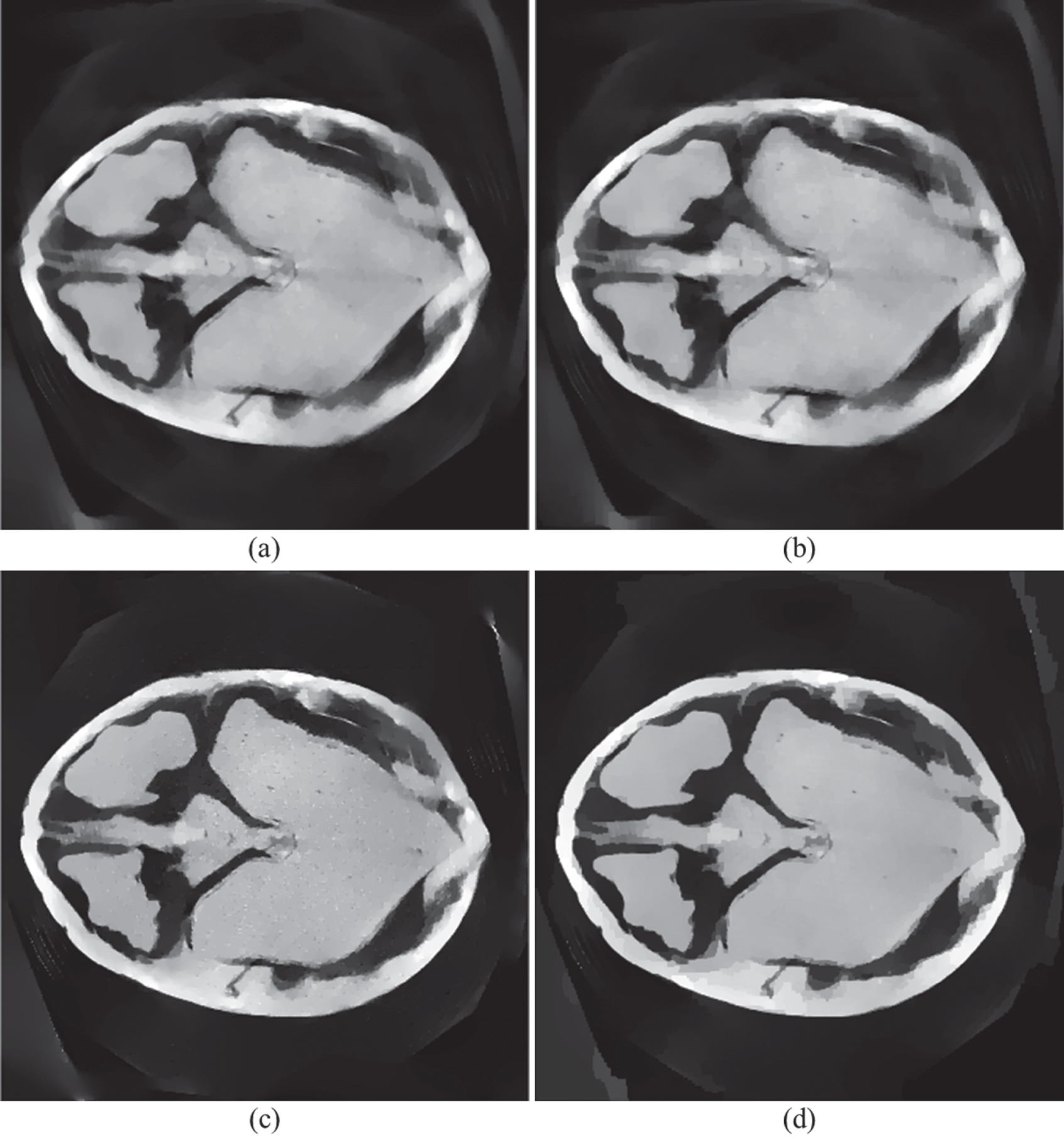
CT images of a walnut reconstructed from projection data in the range of [0°, 30°] ∪ [120°, 150°] ∪ [240°, 270°]. (a) MDTV, (b) wATV, (c) ADM-L0, (d) RTV method. The display window is [0,0.04].

Fig. 22

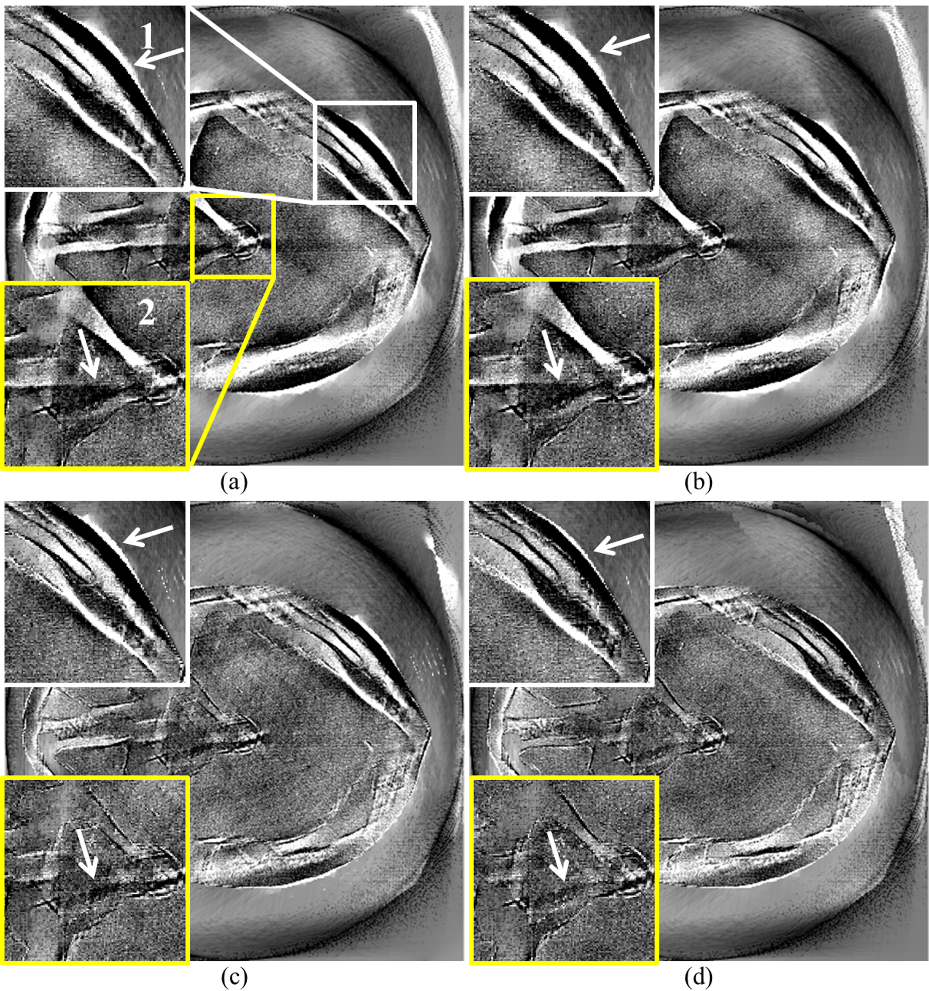
Residual images of different methods related to CT images shown in Figure 21: (a) MDTV, (b) wATV, (c) ADM-L0, (d) RTV method. The display window is [–0.005, 0.005].

4 Discussion and conclusion

This study endeavors to find a practical CT imaging method, including projection data acquisition and image reconstruction. SLA sampling can avoid disadvantages of few-view sampling and limited-angle CT reconstruction. In medical CT, SLA sampling completes projection data acquisition only by switching the tube voltage a few times. This sampling mode can greatly reduce the switching frequency of the tube voltage and can be realized on traditional single-source CT platform without introducing additional cumulative dose. In industrial CT, the combination of SLA sampling and MLCT platform first adapts to the characteristics of batch detection of industrial products so as to improve the throughput of CT system. Besides, it reduces the load of X-ray tube. SLA sampling is expected to become a practical under-sampling scheme. Following this sampling scheme, we have tried to regularize the reconstructed images using multi-direction total variation in our previous work [8]. However, this method cannot reduce the shading artifacts obviously. Hence, in this work, we focus on using the differences between image structures and shading artifacts to regularize CT images, rather than using the direction information of scanning angular range. The used reconstruction method needs to determine some parameter values. Nevertheless, we have given each parameter a relatively fixed reference value to reduce the inconvenience of usage caused by multiple parameters. Although our method outperforms some methods, this CT imaging method including data acquisition and image reconstruction also has its limitations, which needs further consideration and optimization.

First, SLA sampling requires the X-ray source and detector to span a large angular range. For example, in the experiments on FORBILD head phantom, when the projection data is in the range of [0°, 30°] ∪ [120°, 150°] ∪ [240°, 270°], the angular range spanned is at least 270°; when the projection data is in the range of [0°, 30°] ∪ [60°, 90°] ∪ [120°, 150°], the angular range spanned is 150°. The angular range spanned is larger than that in limited-angle CT. In real CT applications, the scanning angular interval is often less than 1 degree to obtain complete projections. The projections at adjacent angles are likely to be redundant. In limited-angle CT, all data samplings are concentrated in one successive angular range. There are many pairs of redundant projections in this range. In SLA CT, data samplings are distributed in multiple successive angular ranges. Although there exist some pairs of redundant projections in each successive range, the angular gap significantly reduces the redundancy of the projections in different angular ranges. Thus, we think acquired SLA CT data has lower data correlation compared to limited-angle CT, which is conductive to reconstructing higher-quality images. Following this idea, we know that few-view sampling in a short-scan angular range can greatly avoid data redundancy. However, compared to few-view sampling, SLA sampling greatly reduces technical requirements of fast switching tube voltage, which collects projection data with low voltage switching frequency and only needs to turn on and off the tube voltage a few times. This mode can be realized on traditional single-source CT platform. Second, because the X-ray source spans a large angular range, SLA sampling may be subject to the geometry of the scanned object. For example, SLA sampling may not acquire the projection data of a long object, since X-rays cannot pass through the long interior of the object at some view angles. In this case, limited-angle CT may be a better choice. Third, the computational time per iteration of MDTV, wATV, ADM-L0, and RTV method are about 0.3147 s, 0.2878 s, 0.3238 s, and 0.5518 s, respectively. The time consumption of our method is slightly larger than other methods. The extra time mainly comes from calculating elements u_x,m, u_y,m, v_x,m, and v_y,m, and solving problem (15) iteratively. Solving the linear equation consumes almost all the time (95%). However, the continuous development of computational power and the power to reduce artifacts and preserve structures offset the potential longer execution time. Besides, the performance of our method is still limited by incomplete projections, new method should be designed to further reduce the shading artifacts.

In conclusion, we present a practical CT imaging method, that is, SLA sampling combined with RTV based CT reconstruction method. And a designed algorithm with two main steps is presented to solve CT reconstruction problem (6). This reconstruction method uses key differences between image structures and shading artifacts to regularize CT images. Experiments on digital phantoms and real CT data indicate that RTV method can obviously reduce shading artifacts.

Footnotes

Acknowledgments

This work is supported by the National Natural Science Foundation of China (61701174), General Project of Chongqing Natural Science Foundation (cstc2021jcyj-msxmX0679), Science and Technology Research Program of Chongqing Education Commission of China (KJQN202000808), and Scientific Research Foundation of Chongqing Technology and Business University (2056023).

References

Zhao

, Zhong

, Xie

et al., Relation between chest CT findings and clinical conditions of coronavirus disease (COVID-19) pneumonia: A multicenter study, American Journal of Roentgenology 214(5) (2020), 1072–1077.

Danala

, Ray

, Desai

et al., Developing new quantitative CT image markers to predict prognosis of acute ischemic stroke patients,, Journal of X-Ray Science and Technology 30(3) (2022), 459–475.

De Chiffre

, Carmignato

, Kruth

J.P.

et al., Industrial applications of computed tomography,, CIRP Annals 63(2) (2014), 655–677.

Guo

, Zeng

, Wang

, Shen

Image reconstruction method for exterior circular cone-beam CT based on weighted directional total variation in cylindrical coordinates,, Journal of Inverse and Ill-posed Problems 28(2) (2020), 155–172.

Manerikar

, Li

, Kak

A.C.

DEBISim: A simulation pipeline for dual energy CT-based baggage inspection systems,, Journal of X-Ray Science and Technology 29(2) (2021), 259–285.

Han

, Bian

, Eaker

D.R.

et al., Algorithm-enabled low-dose micro-CT imaging,, IEEE Transactions on Medical Imaging 30(3) (2011), 606–620.

de González

A.B.

, Darby

Risk of cancer from diagnostic X-rays: Estimates for the UK and 14 other countries,, The Lancet 363(9406) (2004), 345–351.

Abbas

, Lee

, Shin

et al., Effects of sparse sampling schemes on image quality in low-dose CT,, Medical Physics 40(11) (2013), 111915.

Gong

, Zeng

, Guo

et al., Multiple limited-angles computed tomography reconstruction based on multi-direction total variation minimization,, Review of Scientific Instruments 89(12) (2018), 125121.

10.

Chen

, Jin

, Li

, Wang

A limited-angle CT reconstruction method based on anisotropic TV minimization, Physics in Medicine&Biology 58(7) (2013), 2119–2141.

11.

, Wang

, Huang

Edge-preserving reconstruction from sparse projections of limited-angle computed tomography using ℓ0-regularized gradient prior,, Review of Scientific Instruments 88(2017), 043703.

12.

Wang

, Zeng

, Yu

, Xu

Existence and convergence analysis of ℓ0 and ℓ2 regularizations for limited-angle CT reconstruction,, Inverse Problems&Imaging 12(3) (2018), 545–572.

13.

, Zhao

, Li

, Zhang

An image reconstruction model regularized by edge-preserving diffusion and smoothing for limited-angle computed tomography,, Inverse Problems 35(8) (2019), 085004.

14.

Gong

, Zeng

Anisotropic structure property based image reconstruction method for limited-angle computed tomography,, Journal of X-Ray Science and Technology 29(6) (2021), 1079–1102.

15.

Liu

, Wang

, Ritman

E.L.

et al., Image reconstruction from limited angle projections collected by multisource interior X-ray imaging systems,, Physics in Medicine and Biology 56(19) (2011), 6337–6357.

16.

, Yu

, Gong

, Liu

Swinging multi-source industrial CT systems for aperiodic dynamic imaging,, Optics Express 25(20) (2017), 24215–24235.

17.

Shen

, Xing

Multienergy CT acquisition and reconstruction with a stepped tube potential scan,, Medical Physics 42(1) (2015), 282–296.

18.

Wang

, Zhang

, Cai

et al., Multi-segment spectral reconstruction via zero-value set prior, Physics in Medicine&Biology 66(18) (2021), 185006.

19.

Gong

, Zeng

, Wang

Image reconstruction model for limited-angle CT based on prior image induced relative total variation,, Applied Mathematical Modelling 74 (2019), 586–605.

20.

Sidky

E.Y.

, Duchin

, Ullberg

, Pan

A constrained, total-variation minimization algorithm for low-intensity X-ray CT, Medical Physics 38(S1) (2010), S117–S125.

21.

Sidky

E.Y.

, Kao

C.-M.

, Pan

Accurate image reconstruction from few-views and limited-angle data in divergent-beam CT,, Journal of X-Ray Science and Technology 14(2) (2006), 119–139.

22.

Sidky

E.Y.

, Pan

Image reconstruction in circular cone-beam computed tomography by constrained, total-variation minimization,, Physics in Medicine and Biology 53(17) (2008), 4777–4807.

23.

Yang

, Hofmann

, Dapp

et al., TV-based conjugate gradient method and discrete L-curve for few-view CT reconstruction of X-ray data, Optics Express 23(5) (2015), 5368–5387.

24.

Gong

, Zeng

Self-guided limited-angle computed tomography reconstruction based on anisotropic relative total variation,, IEEE Access 8 (2020), 70465–70476.

25.

Needell

, Saab

, Woolf

WeightedA L1-minimization for sparse recovery under arbitrary prior information,, Information and Inference: A Journal of the IMA 6(3) (2017), 284–309.

26.

Wang

, Zeng

, Zhang

et al., An adaptive iteration reconstruction method for limited-angle CT image reconstruction,, Journal of Inverse and Ill-posed Problems 26(6) (2018), 771–787.

27.

Wang

, Wang

, Zhao

et al., Guided image filtering based ℓ0 gradient minimization for limited-angle CT image reconstruction,, Journal of Inverse and Ill-posed Problems 29(4) (2021), 587–598.

28.

, Lu

, Xu

, Jia

Image smoothing via L0-gradient minimization,, ACM Transactions on Graphics 30(6) (2011), 174.

29.

Guo

, Li

, Ma

, Ling

Mutually guided image filtering,, IEEE Transactions on Pattern Analysis and Machine Intelligence 42(3) (2018), 694–707.

30.

, Qiong

, Xia

, Jia

Structure extraction from texture via relative total variation,, ACM Transactions on Graphics 31(6) (2012), 139.

31.

Gong

, Zeng

Adaptive iterative reconstruction based on relative total variation for low-intensity computed tomography,, Signal Processing 165 (2019), 149–162.

32.

Lee

, Lee

, Kim

et al., A feasibility study of low-dose single-scan dual-energy cone-beam CT in many-view under-sampling framework,, IEEE Transactions on Medical Imaging 36(12) (2017), 2578–2587.

33.

Shamul

, Joskowicz

Change detection in sparse CT scans with non-rigid deformations,, Journal of X-Ray Science and Technology 29(6) (2021), 987–1007.

34.

Gao

, Zhang

, Xing

et al., Volumetric imaging from a multisegment straight-line trajectory and a practical reconstruction algorithm,, Optical Engineering 46(7) (2007), 077004.

35.

Zhang

H.M.

, Wang

L.Y.

, Yan

et al., Image reconstruction based on total-variation minimization and alternating direction method in linear scan computed tomography,, Chinese Physics B 22(7) (2013), 078701.

36.

D.J.

, Qu

G.R.

, Hu

C.H.

et al., Anisotropic total variation minimization approach in in-line phase-contrast tomography and its application to correction of ring artifacts,, Chinese Physics B 26(6) (2017), 060701.

37.

Wang

, Zeng

, Yu

et al., An electron beam linear scanning mode for industrial limited-angle nano-computed tomography,, Review of Scientific Instruments 89(1) (2018), 015113.

38.

El Hamidi

, Ménard

, Lugiez

, Ghannam

Weighted and extended total variation for image restoration and decomposition,, Pattern Recognition 43(4) (2010), 1564–1576.

39.

Zhou

, Bovik

A.C.

, Sheikh

H.R.

, Simoncelli

E.P.

Image quality assessment: From error visibility to structural similarity,, IEEE Transactions on Image Processing 13(4) (2004), 600–612.

40.

Bubba

T.A.

, Juvonen

, Lehtonen

et al., Tomographic X-ray data of carved cheese, 2017; arXiv preprint arXiv:1705.05732.

Segmental limited-angle CT reconstruction based on image structural prior

Abstract

Keywords

1 Introduction

2.1 Brief introduction of SLA CT

Table 2 Scanning and reconstruction parameters in simulation experiments Parameter Values Focus-to-object distance (mm) 500 Focus-to-detector distance (mm) 800 Detector Size 512 Length of detector (mm) 512 Reconstructed image size 256×256 Scanning angular interval (degree) 1

Footnotes

Acknowledgments

References

Table 2
Scanning and reconstruction parameters in simulation experiments

Parameter Values

Focus-to-object distance (mm) 500

Focus-to-detector distance (mm) 800

Detector Size 512

Length of detector (mm) 512

Reconstructed image size 256×256

Scanning angular interval (degree) 1