Analytical reconstructions of full-scan multiple source-translation computed tomography under large field of views

Abstract

This paper is to investigate the high-quality analytical reconstructions of multiple source-translation computed tomography (mSTCT) under an extended field of view (FOV). Under the larger FOVs, the previously proposed backprojection filtration (BPF) algorithms for mSTCT, including D-BPF and S-BPF (their differences are different derivate directions along the detector and source, respectively), make some errors and artifacts in the reconstructed images due to a backprojection weighting factor and the half-scan mode, which deviates from the intention of mSTCT imaging. In this paper, to achieve reconstruction with as little error as possible under the extremely extended FOV, we combine the full-scan mSTCT (F-mSTCT) geometry with the previous BPF algorithms to study the performance and derive a suitable redundancy-weighted function for F-mSTCT. The experimental results indicate FS-BPF can get high-quality, stable images under the extremely extended FOV of imaging a large object, though it requires more projections than FD-BPF. Finally, for different practical requirements in extending FOV imaging, we give suggestions on algorithm selection.

Keywords

Multiple source-translation computed tomography extended field-of-view backprojection weighting factor full-scan backprojection filtration

1 Introduction

Micro-computed tomography (Micro-CT) is widely used in the study of object morphology and structure [1–3]. In a lot of scenarios, micro-CT is necessary to image large-sized objects with high resolutions, including larger objects that cannot be cropped, such as some biological samples [4], precious fossils [5], etc., and the demand for high-resolution characterization on a large scale, such as lithium batteries [6, 7]. However, the application of micro-CT is restricted due to its limited field of view (FOV) at high spatial resolution [8]. The main reason is that, in the rotating object-based micro-CT, to avoid truncation artifacts, the object should be completely within the FOV, which is the inner circle of the fan-beam formed by the detector and x-ray source. Therefore, the FOV is mainly limited by the size of the detector, whereas the fabrication of large, inexpensive flat panel detectors remains a challenge. Over the decades, several techniques have been developed to enlarge the FOV, including detector offset [9–11], traverse-continuous-rotate scanning [12], rotation-translation-translation multi-scan mode [13], rotation-translation multi-scan mode [14], elliptical trajectory [15], complementary circular scanning [16], and rotated detector [17]. Previously, Yu et al. [18] proposed a source-translation CT (STCT) to enlarge the FOV in an easier way. To acquire the complete projection data set within the FOV, multiple source-translation CT (mSTCT) was further developed with minimum number of STCT segments with different angles [19]. In mSTCT, the measured object is placed close to the micro-focus x-ray source and far from the detector to achieve a large geometric magnification, and the FOV can be adjusted by just changing the length of the source focus translation. This scanning method of extending the FOV inevitably results in each view being transversely truncated, but the projection data set within the FOV is complete [19]. In FBP-type algorithms, each view is filtered individually, and the truncated projection can introduce infinite high-frequency components in the Fourier domain. Because the actual sampling cannot be infinite, the truncated projection after filtering will generate the Gibbs phenomenon at the truncation point.

To solve this problem, iterative algorithms are effective in obtaining high-quality images, but the reconstruction efficiency is not satisfactory in practice [18]. To avoid the truncation, focusing on effective analytical algorithms, Yu et al. [19] designed a virtual projection-based FBP (V-FBP) algorithm for mSTCT, and the virtual projection is the set of measured x-ray divergents for each detector element. V-FBP performs the ramp-filtering for projection along the source, and the cutoff frequency of the filtering is determined by the number of source sampling points. Hence, a large number of projections need to be acquired to ensure the essential spatial resolution. To directly avoid the truncation, another analytical algorithm, i.e., backprojection filtration (BPF), can be introduced into reconstruction for mSTCT, which is mainly divided into differentiated backprojection (DBP) and finite inversion of Hilbert transform in the image domain. Previously, based on the basic concepts of the BPF algorithm, we derived new BPF algorithms for mSTCT [20]. In this study, we utilized the fact that the detector elements are tightly arranged (i.e., small elements with high resolution) to study the loss of less high-frequency information in mSTCT reconstruction with fewer sampling points. More specifically, the derivative is conducted along the detector and source in DBP, obtaining the D-DBP and S-DBP (the letters “D” and “S” indicate the differentiated operation in DBP, which follows the directions of the detector and the source, respectively) formulas, and finally getting two BPF algorithms for mSTCT, i.e., D-BPF and S-BPF, respectively. The derivative is actually equivalent to special ramp filtering, and the resolution of the detector unit is usually higher than the interval between the source sampling points, so the derivative along the detector has a higher cutoff frequency and keep more high-frequency information. Therefore, D-BPF can reconstruct high-quality image with fewer projections, while S-BPF with derivative along the source requires more projections (this disadvantage is the same as V-FBP).

However, we find that in the larger FOVs, D-BPF reconstructions show unstable, intolerable errors in the area near the source, i.e., some streak artifacts distributed at the edges of the image and FOV. The errors become severe as the FOV and object size increase, which goes against the original purpose of developing mSTCT. Additionally, S-BPF does not generate unstable errors at image edges, but artifacts appear in the reconstructed image as the FOV extends, confirming the issue of the previously proposed redundancy weights for mSTCT.

Zeng et al. [21] proposed the theory of reconstruction error in short scanning of circular trajectories. Inspired by this work, we infer that the backprojection weighting factor in the D-DBP formula is a keyshot that causes unstable errors in mSTCT (it is equivalent to a special short-scan mode). In its backprojection weighting factor and the mSTCT configuration with a large geometric magnification, the distance between the reconstructed point and the source may be a very small value. Especially in extended FOV imaging, if the reconstruction point close to the source is not measured twice, this factor will cause very large errors.

Some existing efforts to eliminate the effect of the backprojection weighting factors are mainly focused on standard scanning trajectories (i.e., circular and helical scans), and some strategies mainly include: the circular harmonic reconstruction (CHR) algorithm [22]; rebinning algorithms, i.e., rebinning projection into parallel beams and then reconstruction [23]; the shift-variant filtering methods in the ramp filter based FBP (rFBP) algorithm [24, 25]; FBP-type algorithm using the Hilbert transform and one-dimensional coordinate transformation between the parallel-beam and fan-beam coordinates, also called hFBP [26]; the shift-variant filtering methods by changing the differential distance when the reconstructed point changes in the Hilbert transform-based FBP-type algorithms [27, 28]; introducing additional weighting in full-scan geometry to eliminate weighting factors with a power of one on rays with complementary angles [23, 29–31]. Among them, hFBP revealed better stability than the rFBP and CHR algorithms [26]. Under most extended FOV and little redundancy situations, FBP-type algorithms are not better than BPF. The fifth method is proven effective in full-scan standard strategies, but it cannot eliminate the weighting factor with quadratic power in the D-DBP formula. In fact, this backprojection weighting factor with a square term is difficult to eliminate and achieve high-quality reconstruction in half-scan mode [27]. In addition, some interesting deep learning methods can also solve this type of problem [32–35].

One relatively simple and feasible motivation is to introduce a full-scan mSTCT geometry, namely F-mSTCT, which may weaken the influence of this unstable weighting factor. To achieve this, we first design a redundancy-weighted function that can effectively adapt to F-mSTCT scanning parameters and then introduce it into the previously proposed S-BPF and D-BPF algorithms, obtaining FD-BPF and FS-BPF (the letter “F” refers to F-mSTCT). The reason why we attempt to perform FD-BPF and FS-BPF in large FOVs separately is that both algorithms have their own advantages. FD-BPF can reconstruct high-quality images with a few projections, but the unstable errors are difficult to balance well as the denominator in the backprojection weighting factor may approach zero with the large FOVs. The denominator in the backprojection weighting factor of S-BPF is the distance value from the reconstructed point to the detector, which will be much larger than that of D-BPF under large geometric magnification, which may result in more stable reconstruction results.

In this paper, our work makes contributions as follows: 1) We propose an optimized redundancy weighting function for F-mSTCT in such a way that the direction of the redundancy weighting for projection can be adjusted according to practical needs; 2) Through numerical experiments, we give some suggestions for F-mSTCT algorithm selection for different extended FOV imaging requirements; 3) We conclude that FS-BPF enables F-mSTCT to extremely enlarge its FOV and reconstruct artifact-free images, surpassing the theoretical maximum FOV extension of commonly used circular trajectory detector-bias CT.

This paper is organized as follows. In Section 2, imaging geometries and BPF algorithms for mSTCT are introduced. Section 3 illustrates our proposed method. Section 4 shows experimental results. Finally, the discussion and conclusion are given in Sections 5 and 6.

2 Preliminaries

2.1 Imaging geometries for mSTCT and F-mSTCT

The mSTCT imaging model is described in Fig. 1(a), which is a half-scan mode and consists of multiple STCTs with gradually increasing angles (θ_n = Δθ · (n - 1), n = 1, 2, … , T, and T is the minimum number of STCTs) [18]. Similar to the half and full scan standard trajectory, we can also introduce the full-scan mSTCT (F-mSTCT) model, as shown in Fig. 1(c).

Fig. 1

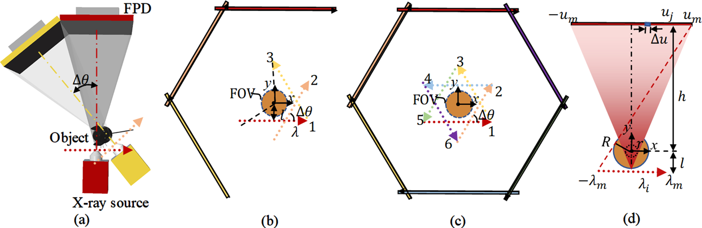
Imaging models: (a) 3D imaging model mSTCT; (b) and (c) are planer imaging geometries of mSTCT and F-mSTCT, respectively; and (d) illustration of each STCT of (b) and (c). The origin of the fixed coordinate system o-xyz is located at the rotated center of the object.

In each STCT, the object is placed close to the source to get a high geometric magnification for the requirement of high resolution, and the source equidistantly and parallelly translates along the row direction of the fixed flat panel detector (FPD) based on the property of the large ray-beam to extend the FOV from the radius r to a larger R (Fig. 1(d)). In mSTCT or F-mSTCT, the complete projection data set within the FOV can be acquired, but each view projection is truncated [18].

In this article, we investigate two-dimensional imaging geometry, and the formula of the source trajectory can be expressed as ${\vec{S}}_{θ_{n}} (λ_{i}) = [λ_{i}, - l] \cdot [\begin{matrix} \cos θ_{n} & \sin θ_{n} \\ - \sin θ_{n} & \cos θ_{n} \end{matrix}],$ (1) where λ_i is the local discrete coordinate of the x-ray source focus (λ is its continuous coordinate), λ_i ∈ [- λ_m, λ_m] (i=1, 2, … , N, N is the number of source sampling points per STCT), λ_m is the half-length of the source translation, and l denotes the origin-to-source distance. u_j is the local discrete coordinate of the x-ray on the detector (u is its continuous coordinate), u_j ∈ [- u_m, u_m] (j = 1, 2, … , J, J is the number of the detector elements), and u_m is the half-size of the detector. The interval angle Δθ between adjacent STCTs meets the relationship: Δθ = 2arctan(u_m/h) (see the original paper [18]), and h is the origin-to-detector distance. In F-mSTCT, T can be determined as T = 2π/Δθ, and ⌈· ⌉ defines rounding numbers upwards. According to the Ref. [18], the calculation of the radius R of the FOV that can acquire the complete projection data set is $R = \frac{λ_{m} h - u_{m} l}{\sqrt{{(l + h)}^{2} + {(λ_{m} + u_{m})}^{2}}} .$ (2)

2.2 BPF-type algorithms for mSTCT

Previously, our research group proposed BPF algorithms for mSTCT, including D-BPF and S-BPF, to avoid the truncation [20]. Therefore, the D-DBP and S-DBP formulas are derived to obtain different DBP images (see Section Introduction, i.e., intermediate images obtained after DBP operations with different differentiated directions), including ${Db}_{η}^{θ_{n}} (\vec{x})$ and ${Sb}_{η}^{θ_{n}} (\vec{x})$ , ${Db}_{η}^{θ_{n}} (\vec{x}) = \frac{1}{2} \int_{- λ_{m}}^{+ λ_{m}} \frac{1}{L^{2}} {\cdot \frac{\partial}{\partial u} {\frac{{(l + h)}^{2} \cdot w_{θ_{n}} (λ, u)}{\sqrt{{(l + h)}^{2} + {(λ - u)}^{2}}} \cdot p_{θ_{n}} (λ, u)} |}_{u = u^{*}} d λ,$ (3) ${Sb}_{η}^{θ_{n}} (\vec{x}) = \frac{1}{2} \int_{- u_{m}}^{+ u_{m}} \frac{1}{H^{2}} {\cdot \frac{\partial}{\partial λ} {\frac{{(l + h)}^{2} \cdot w_{θ_{n}} (λ, u)}{\sqrt{{(l + h)}^{2} + {(λ - u)}^{2}}} \cdot p_{θ_{n}} (λ, u)} |}_{λ = λ^{*}} d u,$ (4) where $\vec{x} = (x, y)$ is the reconstructed point; L = - xsinθ_n + ycosθ_n + l, H = xsinθ_n - ycosθ_n + h; u^* is the local coordinate of the ray from the source focus λ to passing through $\vec{x}$ on the detector, λ^* is the local coordinate of the ray from the detector element u to passing through $\vec{x}$ on the source trajectory. p_{θ
_n} (λ, u) is the projection of the n-th STCT. w_{θ
_n} (λ, u) is a weighting function to eliminate the redundancy data in mSTCT, whose details can be found in the paper [19]. To transform from the DBP image to the object space $f_{θ_{n}} (\vec{x})$ , the inversion of Hilbert transform in the second step needs to be performed for each DBP image along the direction parallel to the source translation [20]. η denotes the angle between the filtering lines of Hilbert transform and the positive y-axis. Finally, overlapping all $f_{θ_{n}} (\vec{x})$ to complete reconstruction within the FOV, i.e., $f_{θ} = \sum_{n = 1}^{T} f_{θ_{n}} (\vec{x})$ .

The previous experiments demonstrated that D-BPF needs fewer projections compared to S-BPF and V-FBP at the same spatial resolution, can reduce source sampling by 75% (e.g., when S-BPF and V-FBP require 1001 projections per STCT, D-BPF only requires 251 projections) [20b]. Since the differential is equivalent to filtering along the detector in D-BPF, its cutoff frequency is influenced by the size and number of elements, whereas others are along the source trajectory and are influenced by the source sampling points.

3 Method

3.1 Problem analysis and strategy

In the mSTCT reconstruction algorithms, our previously proposed D-BPF is verified to be more practical as it significantly improves scanning efficiency and avoids truncation. However, we notice that the reconstructed results within the enlarged FOVs show artifacts. As shown in Fig. 2, these artifacts are exacerbated as the FOV extends, which deviates from the intention of mSTCT imaging. Not only do unstable values appear at the edges, but other artifacts appear in the reconstructed image as the FOV expands. It is significant to improve the reconstruction accuracy under the extreme enlarged FOV, and it may lead to important progress in this field.

Fig. 2

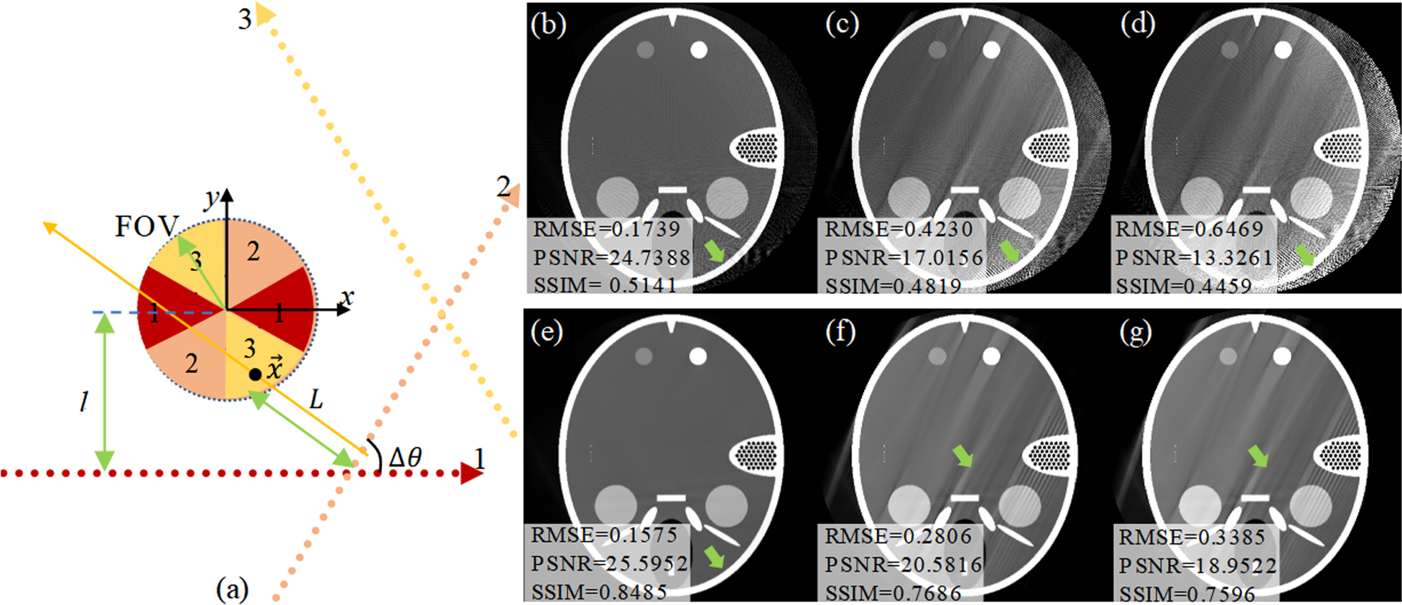
Reconstruction results with the different enlarged FOVs via D-BPF and S-BPF for the half-scan mSTCT imaging geometry consisting of the three-segment STCTs: (a) mSTCT imaging model consists of three-segment STCTs, and the interval between adjacent STCTs is about 62.8°; (b)– (d) reconstructed images when 2λ_m is set to 40 mm, 45 mm, and 50 mm via D-BPF with the number N of source sampling points per STCT being 251, the corresponding radius of the enlarged FOV is 8.3921 mm, 10.1 mm, and 11.77 mm (the half-sizes of the objects are set to them), respectively; and (e)– (g) reconstructed images via S-BPF under the same scanned conditions as (b)– (d) with N being 1001. The reason for the selection of different source sampling points (251 and 1001, respectively) for D-BPF and S-BPF can be found in our previous research [20]. A display window is [0, 3].

Analysis: In F-mSTCT, when not considering redundancy between adjacent STCTs, each reconstructed point is equivalent to being measured twice by complementary rays. Therefore, the errors caused by the factor 1/L² related to the distance from the reconstructed point to the source may be balanced by a value of one far and one near [25, 36]. In the extreme enlarged FOV, there are small values close to zero in the region closer to the source, which makes 1/L² show unstable, intolerable errors and may not be well balanced. Unlike D-DBP, the factor in S-DBP is 1/H², where H denotes the vertical distance from the reconstructed point $\vec{x}$ to the detector. Therefore, the errors generated in S-BPF are theoretically smaller and may be suitable for F-mSTCT reconstruction under the large FOV. Besides, the redundancy weighting established cannot adjust as the FOV of mSTCT extends, so artifacts appear within the reconstructed image from Fig. 2.

Strategy: Attempt to explore the effectiveness and applicability of D-BPF and S-BPF in the F-mSTCT mode (see Fig. 1(c)). The redundancy of F-mSTCT is different from mSTCT, in F-mSTCT, each point to be reconstructed is covered by 360°. However, due to the intersection between source trajectories and detectors, the projections of adjacent STCTs overlap, resulting in redundant projection data and affecting the final reconstruction results. Therefore, we need to derive a redundancy weighting method that is suitable for F-mSTCT and can be adaptively adjusted as the FOV extends. Subsequently, we apply it to D-BPF and S-BPF.

3.2 Redundancy-weighted strategy for F-mSTCT

Inspired by the redundancy-weighted idea in symmetric-geometry computed tomography [37], we analyze and derive the redundant situation and obtained a new redundancy-weighted function applicable to F-mSTCT.

According to the geometric relationship shown in Fig. 3, the projection data p_{θ
_n} (λ, u) of the n-th STCT can be mapped to the equivalent virtual detector that is parallel to the detector past the center of rotation and denoted as q_{θ
_n} (λ, t) one by one. The mapping relationship between p_{θ
_n} (u, λ) and q_{θ
_n} (t, λ) is shown in Equation (5):

Fig. 3

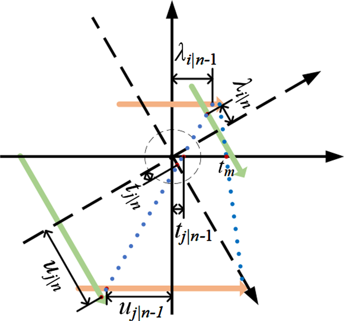
Geometric and schematic of the redundant projection of two adjacent STCTs.

$\begin{matrix} p_{θ_{n}} (λ, u) = q_{θ_{n}} (λ, t), u = \frac{l + h}{l} t - \frac{h}{l} λ \end{matrix}$ (5)

Here, t is the one-dimensional row coordinate of the x-ray on the equivalent virtual detector.

The redundant projection per STCT in F-mSTCT is the same, and the schematic of the redundant projection data of adjacent STCTs is shown in Fig. 3.

Let the range of sampling points of the ray source trajectory be ±λ_m, the range of detector row coordinates be ±u_m, and the maximum range of the virtual detector be ±t_m. t_m is the intersection of the ray represented by (λ_m, u_m) with the t-axis, the maximum value to which t goes, and -t_m is the same as this. All projections of each STCT segment are located within the rectangular coordinate range of [- t_m, t_m] and [- λ_m, λ_m], and the projection data will fill the whole rectangular coordinate range formed by [- t_m, t_m] and [- λ_m, λ_m] when the detector length limitation is not considered.

Then, we mapped the projection data in the t - λ coordinate space to Radon space and redistributed the angular intervals of each STCT segment in Radon space according to the full-scan requirement to obtain the redundancy overlap region between the projection data of two adjacent STCT segments. As shown in Fig. 4(a), in the t - λ coordinate space, the regions A and B of the projection data of the previous STCT segment overlap with the regions A′ and B′ of the later STCT segment, respectively. In addition, a more detailed description of Fig. 4 is in the Supplement.

Fig. 4

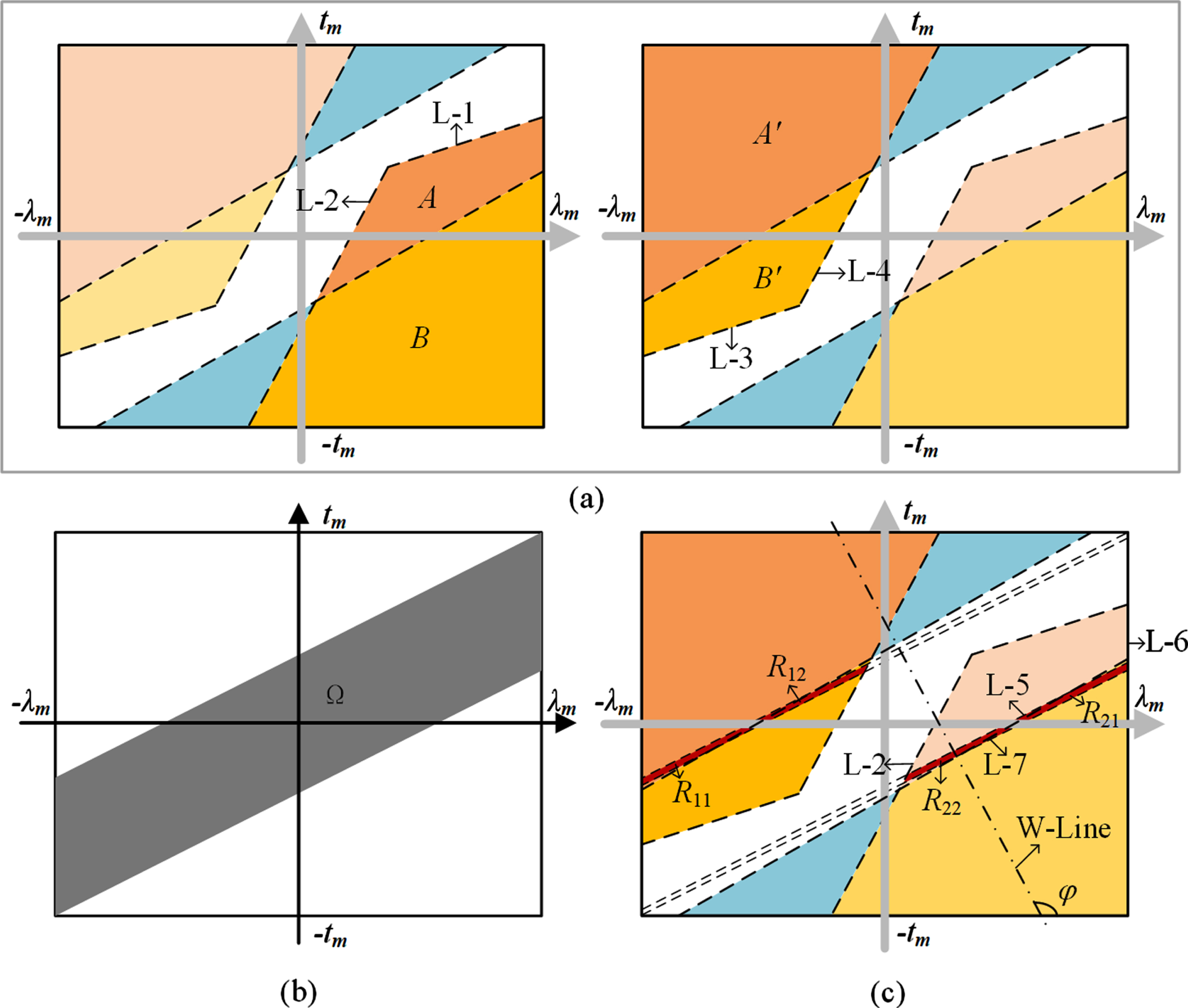
Analysis of the redundant situation for F-mSTCT: (a) a redundant case of two adjacent STCTs in t - λ coordinate space, (b) the effective projection region Ω for each STCT in the t - λ coordinate space, and (c) redundancy-weighted analysis of projection data for STCT.

For the mutually overlapping pair of projection data q_{θ
_n-1} (λ_i|n-1, t_j|n-1) and q_{θ
_n} (λ_i|n, t_j|n) in the redundant regions A, B, A′, B′ shown in Fig. 4(a), there exists the relationship as shown in Equation (6): $\begin{matrix} q_{θ_{n - 1}} (λ_{i | n - 1}, t_{j | n - 1}) = q_{θ_{n}} (λ_{i | n}, t_{j | n}) . \end{matrix}$ (6)

Here, the algebraic relationship between the overlapping projection coordinates (λ_i|n-1, t_j|n-1) and (λ_i|n, t_j|n) shown in Equation (6) satisfies Equation (7). (The detailed derivation of Equation (7) is shown in the Supplement). $\begin{matrix} {\begin{matrix} t_{i | n - 1} = t_{j | n} \sqrt{\frac{{[\frac{(λ_{i | n} - t_{j | n}) l + l^{2} \tan \frac{θ}{2}}{l - (λ_{i | n} - t_{j | n}) \tan \frac{θ}{2}}]}^{2} + l^{2}}{{(λ_{i | n} - t_{j | n})}^{2} + l^{2}}} \\ λ_{i | n - 1} = t_{j | n - 1} + \frac{(λ_{i | n} - t_{j | n}) l + l^{2} \tan \frac{θ}{2}}{l - (λ_{i | n} - t_{j | n}) \tan \frac{θ}{2}} \end{matrix} . \end{matrix}$ (7)

Due to the finite length detector, the projection within the rectangular coordinate range formed by [- t_m, t_m] and [- λ_m, λ_m] in each STCT do not all exist. Only the projection data located within the rectangular coordinate range of [- u_m, u_m] and [- λ_m, λ_m] in the u - λ coordinate space is valid and is mapped to the area Ω in the t - λ coordinate space. Area Ω is called the valid projection (see Fig. 4(b)).

Combining with the valid projection region (Fig. 4(b)), the redundant region of the projection data of one STCT can be obtained, as shown in Fig. 4(c), where the region R₁ (including R₁₁ and R₁₂) is the overlapped redundant region of this segment STCT with the previous segment STCT, and the region R₂ (including R₂₁ and R₂₂) is the overlapped redundant region of this segment STCT with the next segment STCT. For the mutually overlapping pair of projection data q_{θ
_n-1} (λ_i|n-1, t_j|n-1) and q_n (λ_i|n, t_j|n) in the redundant regions R₁₁, R₁₂, R₂₁, R₂₂ shown in Fig. 4(c), they also satisfy the relationship as shown in Equation (6) and Equation (7) as well.

Once the redundant region is determined, the corresponding redundancy-weighted function can be designed. According to the literature [22], the redundancy-weighted function needs to satisfy two conditions: 1) In the redundant region, each point to be reconstructed has only one equivalent x-ray passing through it; 2) The weighting function must be continuous.

As shown in Fig. 4(c), the W-Line is the directional line of redundancy weighting, whose slope tanφ determines the direction of redundancy weighting, and L-2, L-5, L-6, and L-7 are the boundary lines between the redundant region R₂ and the surrounding non-redundant regions. The redundancy-weighted function of the R₂ region is determined by the distance of the projection data points along the direction of the W-Line to the four boundary lines L-2, L-5, L-6, and L-7, and the redundancy-weighted function value of the redundant region R₁ and its corresponding redundancy-weighted function value of the projection data points in the R₂ region in the previous STCT sum to one. In summary, the redundancy-weighted function for the n-th STCT projection data is shown in Equation (8).

$w_{θ_{n}} (λ_{i | n}, t_{j | n}) = {\begin{matrix} 1, & (λ_{i | n}, t_{j | n}) \notin [R_{1}, R_{2}] \\ f (\frac{min ({dis}_{w - 2}, {dis}_{w - 5})}{min ({dis}_{w - 2}, {dis}_{w - 5}) + min ({dis}_{w - 6}, {dis}_{w - 7})}), & (λ_{i | n}, t_{j | n}) \in [R_{2}] \\ 1 - w_{θ_{n - 1}} (λ_{i | n - 1}, t_{j | n - 1}), & (λ_{i | n}, t_{j | n}) \in [R_{1}] \end{matrix} .$ (8)

Here, dis_w-2 denotes the distance of the current projection data point (λ_i|n, t_j|n) along the direction of the W-Line to the L-2 boundary line, and dis_w-5, dis_w-6, and dis_w-7 are the same way. That is, the length of the W-Line passing through the current projection data point (λ_i|n, t_j|n) in the redundant region R₂ is obtained as the denominator, and the distance of the point (λ_i|n, t_j|n) along the direction of the W-Line to the dividing lines L-2 and L-5 is calculated, the smallest of which is taken as the numerator. The ratio obtained above is smoothed by the function f (x) shown in Equation (9) to finally obtain the redundancy weighting function for the redundant region R₂. The redundancy-weighted function of the R₁ region is obtained by calculating the redundancy-weighted function of the R₂ region of the previous section of STCT corresponding to it. (λ_i|n-1, t_j|n-1) and (λ_i|n, t_j|n) in Equation (8) satisfy Equation (7). $\begin{matrix} f (x) = {\begin{matrix} 1, x ⩽ 0 \\ \frac{1 + \sin ((0.5 - x) π)}{2}, 0 < x < 1 \\ 0, x ⩾ 1 \end{matrix} . \end{matrix}$ (9)

Table 1

The pseudo-code for calculating the redundancy-weighted function

Redundancy-weighted function of the n-th STCT
1: Input: ${\hat{w}}_{θ} = 1$ , w_θ = 1, λ_m, u_m.
2: For λ_i\|n = - λ_m : λ_m do
3: For u_j\|n = - u_m: u_m do
4: Calculate t_j\|n by Equation (5);
5: If (λ_i\|n, t_j\|n) ∈ [R₂]
6: Calculate dis_w-2dis_w-5dis_w-6dis_w-7;
7: Calculate w_{θ _n} (λ_i\|n, t_j\|n) by Equation (8);
8: Elseif (λ_i\|n, t_j\|n) ∈ [R₁]
9: Calculate (λ_i\|n-1, t_j\|n-1) by Equation (7);
10: Calculate dis_w-2dis_w-5dis_w-6dis_w-7;
11: Calculate w_{θ _n} (λ_i\|n-1, t_j\|n-1) by Equation (8);
12: Calculate w_{θ _n} (λ_i\|n, t_j\|n) by Equation (8);
13: w_{θ _n} (λ_i\|n, u_j\|n) = w_{θ _n} (λ_i\|n, t_j\|n);
14: End for
15: End for
16: Output: w_{θ _n} (λ_i\|n, u_j\|n).

To illustrate the generation procedure of the proposed redundancy-weighted function and replace w_{θ
_n} (λ, u) in the reconstruction formulas (Equations (3) and (4)) above more visually, Table 1 lists the pseudo-code. Figures 5(a) and (b) show the weighting results of one STCT projection in the t-λ coordinate space and the corresponding u-λ coordinate space, respectively.

Fig. 5

The weighting results when the weighting direction is tanφ = 3π/4: (a) the weighting results of one STCT projection data in the t - λ coordinate space; (b) the weighting results of one STCT projection data in the corresponding u - λ coordinate space. A display window is [0, 1].

4 Experiments

Some numerical experiments are conducted to evaluate our methods. These methods are implemented based on the Astra-Python software tool, and conducted on a computer with an Intel (R) Core i7-8550U CPU @ 1.80 GHz and an NVIDIA GeForce MX250. Table 2 lists scanning parameters, where the length of source translation 2λ_m is set to 40 mm to obtain an enlarged FOV with a radius R of 8.3921 mm (Equation (2)), which exceeds the FOV with a radius r of 6.5402 mm in the standard CT. Additionally, the number T of STCTs in F-mSTCT can be determined to be six, and it is relatively three in mSTCT. The FORBILD phantom, with the size being 2 R×2 R and the reconstructed size being 512×512 pixels, is used to test.

Table 2
Scanning parameters

Parameters Value

Source-to-origin distance l (mm) 13.75

Detector-to-origin distance h (mm) 106.5

Length of source translation 2λ_m(mm) 40

Source sample points per STCT N 251 (D-BPF, FD-BPF, and FW-FBP);

1001 (S-BPF, FS-BPF)

Number of detector elements J 1024

Size of detector element (mm²) 0.127×0.127

Number of STCTs in F-mSTCT T 6

Interval translation angle Δθ (°) 60

Radius of FOV R (mm) 8.3921

Parameters	Value
Source-to-origin distance l (mm)	13.75
Detector-to-origin distance h (mm)	106.5
Length of source translation 2λ_m(mm)	40
Source sample points per STCT N	251 (D-BPF, FD-BPF, and FW-FBP);
	1001 (S-BPF, FS-BPF)
Number of detector elements J	1024
Size of detector element (mm²)	0.127×0.127
Number of STCTs in F-mSTCT T	6
Interval translation angle Δθ (°)	60
Radius of FOV R (mm)	8.3921

As shown in Fig. 6, this experiment can verify effectiveness that the proposed redundancy-weighted function for the F-mSTCT reconstruction.

Fig. 6

Effectiveness illustration of the redundancy-weighted function for the projection in F-mSTCT reconstruction. The display window is [0, 3].

To investigate the performance of FD-BPF and FS-BPF, some experiments are performed under different FOVs, as illustrated in Figs. 7(a)–(c). More specifically, we set 2λ_m to 40 mm, 45 mm, and 50 mm, i.e., the radius of the enlarged FOV is 8.39 mm, 10.1 mm, and 11.77 mm, and the magnification of the FOV is 1.28, 1.54, and 1.8 compared to the standard circular scanning, respectively. In F-mSTCT, we can equate it to detector bias and combine it with smooth redundancy weights to weaken truncation. For this reason, we introduce full scan-weighted FBP (abbreviated as FW-FBP) as a comparison. In the three different FOVs, the reconstructed results, including images and profiles via FW-FBP, FD-BPF, and FS-BPF, are shown in Figs. 7(d)–(g), (h)–(k), and (l)–(o), respectively. The three kinds of metrics, including the root mean square error (RMSE), power signal-to-noise ratio (PSNR) and structural similarity (SSIM), are located at the left-bottom corner of each reconstructed image. The overall error between the reconstructed image and the reference phantom is measured using RMSE. The noise level present in the reconstructed image is measured using PSNR. SSIM is used to assess the similarity between two images. Better reconstruction quality is indicated by a lower RMSE value together with higher PSNR and SSIM values.

Fig. 7

Reconstructed results via FW-FBP, FD-BPF, and FS-BPF under the different enlarged FOVs: (a)– (c) imaging diagrams of different enlarged FOVs; (d)– (f) reconstructed images via FW-FBP under the conditions of (a)– (c); (g) profiles from 0 to 100 pixels in the horizontal center of (d)– (f); (h)– (j) reconstructed images via FD-FBP; (g) profiles of (h)– (j); (l)– (n) reconstructed images via FS-FBP; and (o) the profiles of (h)– (j). The display window is [0, 3].

With the radius of the enlarged FOV being 8.39 mm, FW-FBP can achieve high-quality reconstruction, as shown in Figs. 7(d) and (g). However, as the FOV continuously increases, the images reconstructed through FW-FBP exhibit significant intensity dropouts within the FOV (Fig. 7(g)). Moreover, taking Figs. 2(e)–(g), which show the reconstructed images of D-BPF as references, the reconstruction result of FD-BPF, as originally envisioned, can alleviate the problem of large reconstruction errors. However, as the size of the tested object and FOV increase, some sharp streak artifacts still appear in the reconstructed area near the FOV boundary (Figs. 7(i) and (j)), which are numerically unstable and sharp (Fig. 7(k)) and affect the imaging quality. Thus, FD-BPF still cannot meet the urgent need for high-quality imaging of large objects under large FOVs. In contrast, as shown in Figs. 7(l)–(o) and objective evaluation metrics, FS-BPF can reconstruct high-quality images without visible artifacts, and the profile from 0 to 100 pixels in the central row is close to the truth, even though it requires more projection data (N = 1001) than the two algorithms (N = 251) mentioned above. In high-quality imaging, the issue of reduced efficiency caused by acquiring a large amount of projection data can be accepted.

To further investigate the performance of FS-BPF, we continuously enlarge the FOV and the measured object to let the reconstructed region be extremely close to the source trajectory, as described in Figs. 8(a)–(c). More specifically, 2λ_m is set to 52 mm, 54 mm, and 55 mm, corresponding to the radius of the FOV being 12.4318 mm, 13.0855 mm, and 13.4102 mm, and the magnification of the FOV is about 1.9, 2, and 2.05 compared to the standard circular scanning, respectively. Figures 8(d)–(f) display the reconstructed images and three metrics corresponding to the conditions of Figs. 8(a)–(c), and Fig. 8(g) shows the profile from 350 to 512 pixels in the horizontal center of three images. Besides, we also choose a medical CT slice with 512×512 pixels as the tested object. With N being 1201, the high-quality reconstructed results are presented in Figs. 8(h)–(k) without visible artifacts, even though the reconstructed regions are extremely close to the source.

Fig. 8

Reconstructed results via FS-BPF under the extended FOVs where the reconstruction area is extremely close to the source trajectory: (a)– (c) imaging diagrams of different enlarged FOVs; (d)– (f) reconstructed images under the conditions of (a)– (c); (g) profiles from 350 to 512 pixels in the horizontal center of (d)– (f); (h)–(j) reconstructed images for a medical phantom; and (k) horizontal central profiles of (h)–(j). The window ranges are [0, 3] and [90, 150] (HU) for the FORBILD phantom and medical phantom, respectively.

5 Discussion

Aiming at solving the problem of reconstruction errors under the large FOVs of mSTCT and extending the FOV as much as possible to achieve high-quality imaging, we propose FD-BPF and FS-BPF by constructing F-mSTCT and corresponding to the redundancy weights.

When the FOV is extended infinitely close to the source, FS-BPF still obtain satisfactory reconstructed images even though it requires a large number of projections. Impressively, when the FOV is extended to 2.05 times, the reconstruction results of FS-BPF remain stable. In fact, the result can demonstrate the F-mSTCT reconstruction breaks through the theoretical maximum limit of two times for detector bias expansion FOV imaging methods (the two times are only theoretical values, and practical high-quality imaging is less than two times due to the requirement for enough redundancy).

From the numerical experimental results, we can preliminarily conclude the following:

When the amplification of the FOV only needs to be less than about 1.28 (i.e., the FOV is slightly enlarged), we can use FW-FBP to reconstruct and keep scanning efficiency;

When amplifying FOV requires a range of 1.28–1.54 times and higher scanning efficiency is needed, FD-FBP can be used to reconstruct;

When amplifying FOV exceeds 1.54 times and there is no concern for scanning efficiency, FS-BPF can be used to reconstruct better-quality images.

5.1 Differences on the redundancy weighting for mSTCT and F-mSTCT

Compared with the redundancy-weighted function for mSTCT, our proposed redundancy weighting method has the following advantages:

It has a simpler redundancy profile with only one type of redundancy, whereas the proposed method in mSTCT [19] has three types of redundancy and a more complex redundancy profile;

The redundancy from the geometric relationship between the ray source and the detector was analyzed in mSTCT, while the redundancy of the projection after mapping the projection to the Radon space was analyzed in our proposed method, which makes the process of deriving the redundant region of projection data more accurate and clear;

We optimize the weighting of the redundant projection data in such a way that the direction of the redundancy weighting can be adjusted, which cannot be achieved by the previous weighting method [19] (see reconstructed results in Fig. 2). More specifically, the paper [19] determined the projection redundancy in u-λ coordinate space based on the location of the intersection of one STCT projection line with the source trajectory and detector of an adjacent STCT. It is proven that the redundant region extraction method described in this paper is basically consistent with the redundant regions extracted by this method, and both achieve quite accurate redundant region extraction. Additionally, when designing the redundancy-weighted function, its method is to calculate the redundancy-weighted function by directly calculating the distance from the projection coordinate point to the corresponding redundancy boundary, and the weighting direction and effect are fixed, while in this paper, a W-Line is added as the weighting direction line, which makes the weighting direction adjustable and thus ensures the smooth continuity of the redundancy-weighted function at the boundary under different scanning parameters and then obtains a better reconstruction effect.

5.2 Analysis of reconstruction differences among these methods

Taking F-mSTCT to be equivalent to the detector bias system, FW-FBP utilizes the idea of the weighted FBP to weaken the truncation. Due to a global ramp filter, the truncation error will affect the whole filtered data if the smooth curve for redundant projection is narrow. When 2λ_m≤40 mm, FW-FBP gets competitive results, whereas its errors significantly increase with 2λ_m being greater than 40 mm. The phenomenon of two boundaries being simultaneously truncated may occur with the enlarged size of the FOV and object. In this case, directly using the weighted FBP idea of detector bias (usually truncation only occurs on one side) may not be suitable.

FD-BPF can weaken the unstable errors in areas where the reconstructed points are close to the source. However, as the FOV and reconstructed object are extremely enlarged, the distance parameter L in the backprojection weighting factor 1/L² approaches zero in the region near the source, which leads to highly unstable weighted values that are difficult to be balanced by complementary rays.

In the reconstructed area near the source, the distance parameter H in the backprojection weighting factor 1/H² of FS-BPF is much larger than L due to the high magnification. Therefore, the weighting factor 1/H² has a weak impact on reconstruction errors. Additionally, the projection of one STCT is non-truncated along the source trajectory, which will not produce errors at the truncation points after the finite difference like FD-BPF. Even with the requirement of large projection data, FS-BPF can obtain high-quality images when the FOV is extremely extended and close to the source.

6 Conclusion

In the half-scan mSTCT reconstruction, the backprojection weighting factors cause artifacts and errors as the FOV and object size increase. Besides, the existing redundancy weighting for mSTCT is not working well with adjusting FOVs. To this end, we combine the F-mSTCT geometry with the BPF algorithms to propose FD-BPF and FS-BPF, and design a redundancy-weighted function that can adaptively adjust according to the F-mSTCT geometry. The experiments demonstrate that FS-BPF has the ability to reconstruct high-quality images using large amounts of projection data, even if the extended FOV is extremely close to the source. Finally, according to the different practical requirements for extended FOVs, we provide suggestions on how to choose a reasonable analytical algorithm.

Footnotes

Funding

This research work is supported by Nationa National Natural Science Foundation of China (52075133) and CGN-HIT Advanced Nuclear and New Energy Research Institute (CGN-HIT202215). Authors thank Prof. Fenglin Liu and Dr. Haijun Yu in the Engineering Research Center of Industrial Computed Tomography Nondestructive Testing, Ministry of Education, Chongqing University, for selflessly providing me with learning materials on mSTCT and its reconstruction algorithms.

Disclosures

The authors declare no conflicts of interest.

Data availability

Data underlying the results presented in this paper can be obtained from the authors upon reasonable request.

References

Chung

S.-Y.

, Kim

J.-S.

, Stephan

, Han

T.-S.

Overview of the use of micro-computed tomography (micro-CT) to investigate the relation between the material characteristics and properties of cement-based materials, Constr Build Mater 229 (2019), 116843.

Huang

, Causse

, Brailovski

, Hu

, Trochu

Reconstruction of mesostructural material twin models of engineering textiles based on Micro-CT Aided Geometric Modeling, Compos Part Appl Sci Manuf 124 (2019), 105481.

Wang

, Miller

Current developments and applications of micro-CT for the 3D analysis of multiphase mineral systems in geometallurgy, Earth-Sci Rev 211 (2020), 103406.

Du Plessis

, Broeckhoven

, Guelpa

and Le Roux

S.G.

, Laboratory x-ray micro-computed tomography: a user guideline for biological samples, Gigascience 6(6) (2017), gix027.

Stübling

E.-M.

, Rehn

, Siebrecht

, Bauckhage

, Öhrström

, Eppenberger

, Balzer

J.C.

, Rühli

, Koch

Application of a robotic THz imaging system for sub-surface analysis of ancient human remains, Sci Rep 9(1) (2019), 3390.

Müller

, Sauter

, Shunmugasundaram

, Wenzler

, De Andrade

, De Carlo

, Konukoglu

and Wood

, Deep learning-based segmentation of lithium-ion battery microstructures enhanced by artificially generated electrodes, Nat Commun 12(1) (2021), 6205.

, Bertei

, Finegan

D.P.

, Tan

, Daemi

S.R.

, Weaving

J.S.

, O’Regan

K.B.

, Heenan

T.M.

, Hinds

, Kendrick

and others, 3D microstructure design of lithium-ion battery electrodes assisted by x-ray nano-computed tomography and modelling, Nat Commun 11(1) (2020), 2079.

Yakovlev

M.A.

, Vanselow

D.J.

, Ngu

M.S.

, Zaino

C.R.

, Katz

S.R.

, Ding

, Parkinson

, Wang

S.Y.

, Ang

K.C.

, La

Riviere and others, A wide-field micro-computed tomography detector: micron resolution at half-centimetre scale, J Synchrotron Radiat 29(2) (2022), 505–514.

Sharma

K.S.

, Gong

, Ghasemalizadeh

, Yu

, Wang

, Cao

Interior micro-CT with an offset detector, Med Phys 41(6Part1) (2014), 061915.

10.

Lin

, Yang

, Wu

, Tang

, Zhang

A reconstruction method through projection data conversion under the displaced detector scanning for industrial cone-beam ct, IEEE Trans Nucl Sci 66(12) (2019), 2364–2378.

11.

Herbst

, Schebesch

, Berger

, Choi

J.-H.

, Fahrig

, Hornegger

, Maier

Dynamic detector offsets for field of view extension in C-arm computed tomography with application to weight-bearing imaging, Med Phys 42(5) (2015), 2718–2729.

12.

Nahamoo

, Crawford

C.R.

, Kak

A.C.

Design constraints and reconstruction algorithms for traverse-continuous-rotate CT scanners, IEEE Trans Biomed Eng (1981);(2):79–98.

13.

, Chen

, Zhang

A new reconstruction algorithm for cone-beam CT with unilateral off-centered RT multi-scan, in Industrial and Applied Mathematics in China (World Scientific, 2009) pp. 215–228.

14.

Chen

, Zhang

BPF-based reconstruction algorithm for multiple rotation– translation scan mode, Prog Nat Sci 18(2) (2008), 209–216.

15.

, Li

, Yang

, Heron

D.E.

, Huq

M.S.

A novel off-axis scanning method for an enlarged ellipse cone-beam computed tomography field of view, Med Phys 37(12) (2010), 6233–6239.

16.

Yang

, Li

, Goddu

S.M.

, Tan

CBCT volumetric coverage extension using a pair of complementary circular scans with complementary kV detector lateral and longitudinal offsets, Phys Med Biol 59 (2014), 6327–6339.

17.

Stromer

, Kugler

, Bauer

, Lauritsch

, Maier

A.K.

Data Completeness Estimation for 3D C-Arm Scans with Rotated Detector to Enlarge the Lateral Field-of-View, in Für Die Medizin (2016), pp. 164–169.

18.

, Li

, Tan

, Liu

, Zhou

x-ray source translation based computed tomography (STCT), Opt Express 29(13) (2021), 19743–19758.

19.

, Ni

, Chen

, Ge

, Zhang

, Liu

Analytical reconstruction algorithm for multiple source-translation computed tomography (mSTCT), Appl Math Model 117 (2023), 251–266.

20.

Wang

, Yu

, Huang

, Wang

, Ni

, Li

, Liu

, Cui

BPF Algorithms for Multiple Source-Translation Computed Tomography Reconstruction, arXiv, arXiv:2305.18878 (2023).

21.

Zeng

The fan-beam short-scan FBP algorithm is not exact, Phys Med Biol 60(8) (2015), N131.

22.

Parker

D.L.

Optimal short scan convolution reconstruction for fan beam CT, (2), Med Phys 9 (1982), 254–257.

23.

You

, Zeng

G.L.

Hilbert transform based FBP algorithm for fan-beam CT full and partial scans, IEEE Trans Med Imaging 26(2) (2007), 190–199.

24.

You

, Liang

, Bao

A harmonic decomposition reconstruction algorithm for spatially varying focal length collimators, IEEE Trans Med Imaging 17(6) (1998), 995–1002.

25.

Pan

, Yu

Image reconstruction with shift-variant filtration and its implication for noise and resolution properties in fan-beam computed tomography, Med Phys 30(4) (2003), 590–600.

26.

Wang

, Lu

, Li

, Liang

An alternative solution to the nonuniform noise propagation problem in fan-beam FBP image reconstruction, Med Phys 32(11) (2005), 3389–3394.

27.

Dennerlein

, Noo

Avoiding the backprojection weight in short-scan CT reconstruction, in 2009 IEEE Nuclear Science Symposium Conference Record (NSS/MIC) (IEEE, 2009) pp. 2507–2509.

28.

Dennerlein

, Kunze

, Noo

Filtered Backprojection Reconstruction with Depth-Dependent Filtering, Tsinghua Sci Technol 15 (2010), 17–24.

29.

Narasimhadhan

A.V.

, Rajgopal

FDK-type algorithms with no backprojection weight for circular and helical scan CT, Int J Biomed Imaging 2012 (2012).

30.

Xia

, Cho

, Pan

Backprojection-filtration reconstruction without invoking a spatially varying weighting factor, Med Phys 37(3) (2010), 1201–1209.

31.

Dennerlein

, Noo

, Hornegger

, Lauritsch

Fan-beam filtered-backprojection reconstruction without backprojection weight, Phys Med Biol 52(11) (2007), 3227.

32.

, Hu

, Niu

, Yu

, Vardhanabhuti

, Wang

DRONE: Dual-Domain Residual-based Optimization NEtwork for Sparse-View CT Reconstruction, IEEE Trans Med Imaging 40(11) (2021), 3002–3014.

33.

, Guo

, Chen

, Wang

, Chen

Deep Embedding-Attention-Refinement for Sparse-View CT Reconstruction, IEEE Trans Instrum Meas 72 (2023), 1–11.

34.

Zhang

, Liu

, Yu

, Dong

MetaInv-Net: Meta Inversion Network for Sparse View CT Image Reconstruction, IEEE Trans Med Imaging 40(2) (2021), 621–634.

35.

Okamoto

, Ohnishi

, Haneishi

Artifact Reduction for Sparse-View CT Using Deep Learning With Band Patch, IEEE Trans Radiat Plasma Med Sci 6(8) (2022), 859–873.

36.

Zeng and G.L , Nonuniform noise propagation by using the ramp filter in fan-beam computed tomography, IEEE Trans Med Imaging 23(6) (2004), 690.

37.

Zhang

, Xing

Zhang

, Jin

, Gao

and Chen

, Stationary Computed Tomography with Source and Detector in Linear Symmetric-Geometry: Direct Filtered-Backprojection Reconstruction, Med Phys 47 (2020).