Resolution analysis of a volumetric coded aperture X-ray diffraction imaging system

1 Introduction

X-ray diffraction (XRD), considered the gold standard for the non-destructive analysis of material composition [1], can provide highly accurate information about the molecular makeup of a material. This information is particularly useful in tasks related to discriminating between materials of nearly identical densities and chemical compositions [2–6]. X-ray diffraction imaging (XRDI) involves measuring the XRD signal in a spatially-resolved manner from a 2D or 3D volume [7–10]. This XRDI approach extends the relevance of XRD-based analysis to a wide range of applications [9, 11–14], as many situations require evaluating samples for which spatial correlations must be preserved and traditional ‘nondestructive’ sample preparation methods (such as crystallization or powderization) cannot be implemented [2, 5]. Coded-aperture XRDI (CA-XRDI), in which a detector-side spatial modulation is imposed on the scatter signal to encode scatterer location, is an exciting technology due to its ability to increase useful photon throughput, capture energy-dispersive and angle-dispersive XRD signals, measure large fields of view for fast acquisitions, and be geometrically variable to better suit a wide variety of experimental needs. However, the resolution theories present in the literature are inconsistent with one another, are often vague in their definitions of how resolution is defined, and lack validation across various parameters and their impact on system performance, particularly in the case of 3D imaging.

More specifically, MacCabe et al. [15] developed a resolution estimate for a system involving fan beam illumination and a 2D coded aperture. However, this work assumed that the scatter signal was isotropic and therefore did not apply directly to the structured, small angle scatter signal produced in XRD [15]. Hassan et al. [16] extended the theory of MacCabe et al. to account for a limited angular extent of the scatter signal and included energy-resolved measurements. However, that study was validated using a simple object placed at a single location in the system’s field of view (FOV) and with only a 1D coded aperture and linear detector array [16]. Stryker et al. [9] showed that this theory was consistent with experimental measurements made using a 2D coded aperture, but the study was limited to imaging of 2D projections of thin objects in a single scanning plane.

In this paper, we review existing theories, present a quantitative, self-consistent framework, and validate the models experimentally for CA-XRDI resolution using a home-built three-dimensional coded aperture XRD imaging system [9]. Furthermore, we show that while no single theory is completely accurate, consideration of multiple theories and their context can provide reasonable estimates of resolution throughout a broad range of parameters.

2 Theory

A coded aperture is an attenuating object with a pattern of spatially varying opacity that modulates the signal passing through in a manner that is agnostic of incident angle. Independent scatter points within the field of view of the aperture project unique shadows onto the detector depending on their unique location. If two isotropic sources are laterally separated along the y axis (Δy) as shown in Fig. 1, the code modulations projected onto the detector undergo a shift proportional to the lateral displacement of the scatterer. If separated along the depth direction of the z axis (Δz) shown in Fig. 1, the shadow of the coded aperture is magnified by a factor proportional to the location along z. These are the basic concepts from which prior studies [15, 16] derive their transverse and depth resolution theories.

OPEN IN VIEWER

Fig. 1

Schematic of the experimental setup used in this work. The fan beam is in the y-z plane. The sample is scanned along the x axis at each of the four discrete z_o values to create four unique data sets. The coded aperture and detector are parallel to one another and extend along the x-y plane. In the experiment depicted, the source-to-sample distance (z_o) is 460 mm, the source-to-coded aperture distance (z_m) is 534 mm, and the source-to-detector distance (z_d) is 633 mm. z_m and z_d are constant for all experiments in this study. Depicted at the detector is a coded-aperture modulated Debye ring representing the weighted average momentum transfer value ( q ¯ w ) of the form factor, f (q). L shows the effective detector length, defined as the extent needed to measure f( q ¯ w ), which is deflected by the weighted average angle of θ ¯ w .

In both the Hassan [16] and MacCabe [15] studies, the transverse resolution, Δy _min , of a CA-XRDI system can be estimated using Equation (1) Δ y min = ν ( z d - z o ) ( z d - z m )(1) where ν is the code feature size, z_d is the distance from source to detector, z_o is the distance from source to object, and z_m is the distance from source to the coded aperture. The orientation of the axis and locations of elements are shown in Fig. 1. This equation was derived by considering two points as resolvable only if their separation in y corresponds to a shift of the coded aperture pattern on the detector by the extent of one whole code feature. Although both studies arrive at this resolution relationship, we will refer to this as the Hassan transverse resolution theory.

Equation (1) assumes that the scatter is isotropic and that all spatial information about the scatter’s origin comes from the shadow of the code itself. However, this is not the case for XRD, in which the scatter from each lattice spacing gives rise to a highly structured, non-isotropic signal. For example, non-crystalline materials, such as the one used in this work, and powdered materials both give rise to Debye rings. These rings correspond to an azimuthally-symmetric cone whose apex is the initial scattering location, which can provide additional spatial resolution beyond code feature shifts from isotropic scatter. The Hassan theory of Equation (1) is an overly conservative estimate of resolution since it does not consider the structured and/or limited angle scatter, as is the case for the XRD signal. However, making use of the Debye ring structure described above necessitates a more thorough analysis that considers the energy spectrum of the source, the energy resolution of the detector (if applicable), the breadth of a scattering signal and the detector pixel noise characteristics.

A more simplistic approximation of transverse resolution that includes the case of a Debye-ring-structured signal can be calculated by using similar triangles and calculating the lateral distance that a point source would have to move to shift the Debye-ring structure by one detector element. We consider this single pixel shift of the Debye ring as a minimum requirement for detectability in the transverse resolution dimension, as opposed to requiring one code feature shift at the detector, as in the Hassan theory. This equation will be referred to as the geometric theory, due to its simple use of geometry, and takes the form of Equation (2) below, where p represents the detector’s pixel pitch, and all other variables are the same as Equation (1). Δ y min = p ( z m - z o ) ( z d - z m )(2)

This would represent an idealized transverse resolution in the case of a noiseless detector and perfect knowledge of the photon’s energy. Knowing this is not the case in our experiment, this relationship will be used as setting the floor for the smallest possible resolution. We would expect our measured resolution to be somewhere between the predictions of Equations (1) and (2).

To evaluate the depth resolution, Ref. [16] derives Equation (3) where Δz_min is the minimum resolvable scatterer separation along z, and L is defined as the effective detector length, described more thoroughly below. Δ z min = 2 v ( z d - z o ) 2 ( z d - z m ) L(3)

The depth resolution presented in Ref. [16] differs by a factor of two from the equation given by Ref. [15] in Equation (4) Δ z min = ν ( z d - z o ) 2 ( z d - z m ) L(4)

The factor of two difference between Equations (3) and (4) comes from a choice in defining resolution based on a coded aperture shadow magnification of one code feature (a Ɖ coded-aperture period) at the detector, or a magnification of a full period at the detector (i.e. one open feature and one closed feature), which requires the factor of two. The effective detector length, L, along with the code feature size (which is inversely related to the code frequency), determines the number of code modulations observed at the detector. Using Fourier analysis of a finite-duration signal, one finds that the minimum resolvable depth resolution is directly related to the number of measured code modulations at the detector. Similar to the transverse equations, the Ref. [16] depth resolution equation is likely a conservative estimate, which would predict a larger depth resolution than experimental data may suggest.

In both Equations (3) and (4), the value of L can be slightly ambiguous, and how it is applied is dependent upon the experiment itself. We clarify its role and interpretation here to help provide consistency and applicability of the theories. L corresponds to the extent over which a particular Debye ring, modulated by the coded aperture, covers the detector.

The extent of the coverage depends on the deflection angle of the scattered signal, which is determined by the momentum transfer of the coherent scatter, the location in the FOV of the interaction, and the incident photon’s energy. The relationship between energy and deflection angle is given by Bragg’s law as the momentum transfer value, q. We define q in the same manner seen in the work by Greenberg in Ref. [1], Hassan et al. in Ref. [16] and Stryker et al. in Ref. [17]. q = 1 2 d = E hc sin ( θ 2 )(5)

Here, d is the effective lattice spacing for crystalline materials (and represents average molecular spacing for non-crystalline materials), E is the incident photon energy, h is Planck’s constant, c is speed of light, and θ is the deflection angle. We now have a way to convert between a measured Debye ring’s scattering angle and the momentum transfer of the scatter when the incident photon’s energy is known.

It should be noted that a scattering object usually does not produce a single scattering ring, but often a structured, continuous distribution of intensity across momentum transfer values. We refer to this scattering intensity modulation as the form factor, f (q), which is the square of the conventional modulation to the scattering field, F (q). Form factors are unique for each material and are the source of material specificity in XRD techniques. They can present as a multitude of narrow rings with varying intensity, or as broad sloping structures, or even a combination of the two. Coherently scattered X-rays are the primary cause of this unique structure, which is why from here forward the term “form factor” will specifically be referencing coherent scatter component of our measured signal. To make our use of L generalizable across both a variety of system architectures and sample materials, we define our Debye ring extent at the detector based on the weighted average momentum transfer value, q ¯ w , calculated from the measured f (q). q ¯ w = ∑ ( I i * q i ) ∑ I i(6)

I _i represents the intensity (I) of the normalized scatter signal at each interval (i). In Equation (6), the range and intervals of the summations are derived from the range of q values our system measures, and the q-resolution used in our reconstruction models. For our system, the range for q is between 0.05 and 0.4 Å^–1 (0.5–4 nm^–1), with intervals steps of 0.01 Å^–1. We can use this weighted average momentum transfer value ( q ¯ w ) to calculate the weighted average deflection angle ( θ ¯ w ) by adjusting Equation (5) to read as q ¯ w = 1 2 d = E hc sin ( θ ¯ w 2 ) .

By converting the continuous distribution of a form factor to a single value of the weighted average deflection angle ( θ ¯ w ) , and using 60 keV for E due to this being the dominant incident photon energy from our source [17], we can calculate a single value of L using trigonometry and the known geometry of each experimental configuration, as depicted in Fig. 1, to derive Equation (7). L = 2 * ( Z d - Z o ) * tan ( θ ¯ w )(7)

The weighted average momentum transfer value for the material used in this study (polylactic acid, or PLA) was 0.22 Å^–1. Therefore, for Z_o values of 310, 360, 410, and 460 mm, we have calculated L values of 58.8, 49.7, 40.6, and 31.5 mm respectively. Combining these L values with Equations (3) and (4) gives the two resolution values which set the bounds for our expected experimentally measured resolution value for each experiment, as seen in Table 1. It should be noted that L is geometrically dependent, and that this calculation assumes the depth in the sample at which the scatter interaction takes place. Furthermore, since the value of L changes based on the weighted average of a sample’s form factor, and a change in L would change the depth resolution calculation, these definitions imply that for a fixed geometry resolution is also material-dependent.

In the experiment described in this paper, we used a coded aperture with a 2D random code and a signal dominated by X-rays at 60 keV [17], and focused on coherent scatter angles that ranged between the typical regimes of small-angle X-ray scatter (SAXS) and wide-angle X-ray scatter (WAXS). This gives a range of momentum transfer values between q = 0.05 and q = 0.4 Å^–1 with a resolution of Δq = 0.01 Å^–1.

Using Equations (1–4) and the varying geometries of this experiment, we calculated the expected resolution values in both the transverse and depth dimensions using each of the approximate relations above. Table 1 Displays the calculated expected resolution values for both the transverse and depth directions using each of the theories described above. The values are in millimeters and serve as ‘rule of thumb’ values that may be expected in this experiment, which helped guide our choices in gap width when designing the PLA phantoms.

The CA-XRDI system used in this experiment is shown schematically in Fig. 1. It was designed to scan thin biological samples over a lateral FOV of 15×15 cm with a scan time on the order of 10’s of minutes [9]. The system employs a stationary X-ray primary fan-beam with a sample stage that linearly translates the sample through the beam (i.e., orthogonal to the plane of the fan). The X-ray source is a tungsten anode Monoblock source (XRB160x4111, Spellman) with a 0.5 mm focal spot and typically operated at 160 kV and 3 mA. The detector is a Xineos-2329, made by Teledyne DALSA [18], which is located in the x-y plane at a distance of 630 mm from the source focal spot (z_d). A 2D random-feature coded aperture [17] oriented parallel to the detector surface is situated between the detector and sample stage, as shown in Fig. 1. The coded aperture is 530 mm above the source (z_m) and displays a 2D random pattern of open and closed features, either of which have a minimum width of 0.75 mm, and an open-to-close ratio of 40-to-60% respectively. The sample is placed at either 310, 360, 410, or 460 mm above the source (z_o) for each experimental configuration. The lowest sample location, z_o = 310 mm,.

The system was designed for scanning thin (<1 cm thick) samples at z_o = 310 mm, which corresponds to the configuration used by Stryker et al. [9]. To explore the system performance at a range of different sample scanning planes, we designed elevated sample stages to allow for changing the sample scanning plane without impacting any other aspects of the measurement. These stages, shown in Fig. 2, incorporate the same platform material as the original setup (i.e., thin sheet of radiochromic film) and avoid any additional structures in the fan beam that might introduce additional scatter. Three additional stages were constructed to allow for the four sample scanning locations stated above (z_o = 310, 360, 410, and 460 mm).

OPEN IN VIEWER

Fig. 2

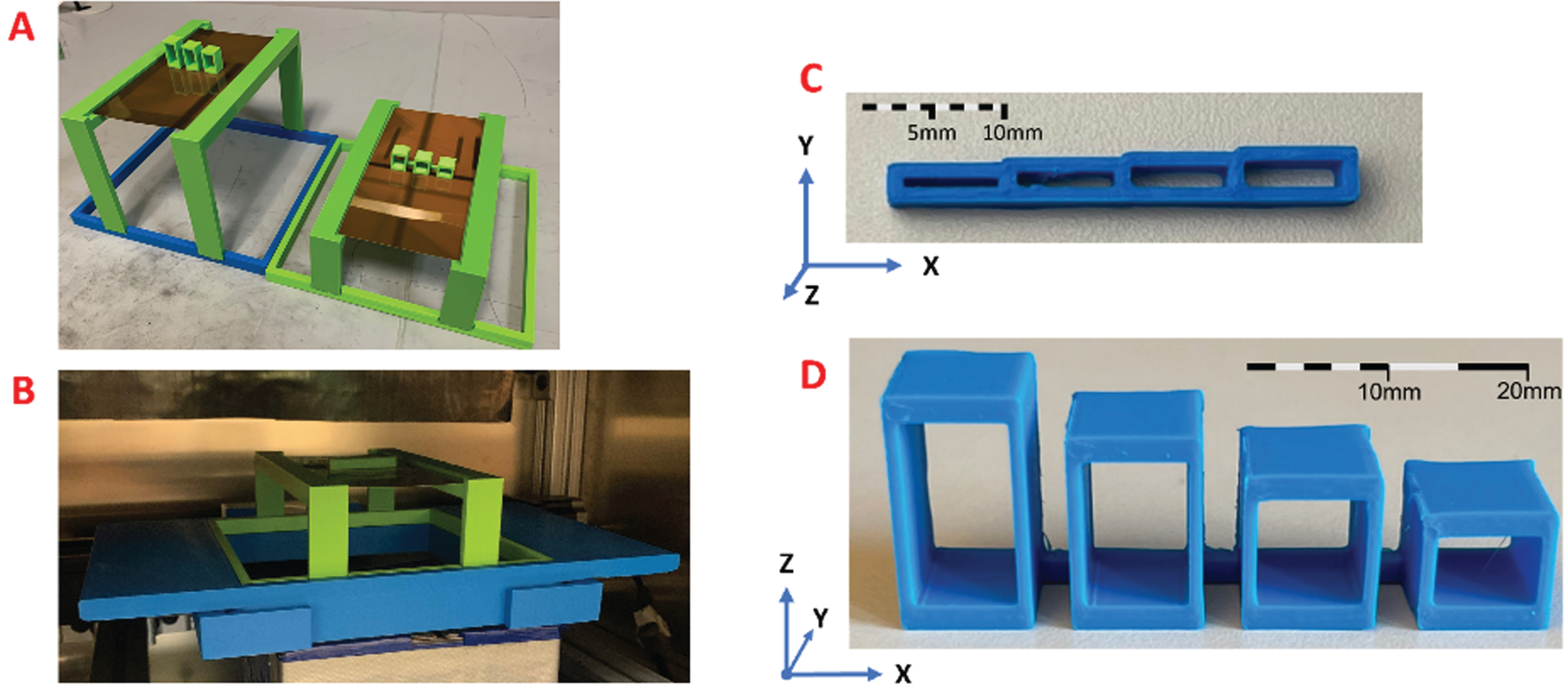
Depiction of 3D printed stages and the resolution phantoms used in this study. A) shows the 5 and 10 cm height stages next to each other with example phantoms placed on the object stage. B) shows how the 5 cm stage fits in the original sample holder to create an elevated surface inside the XRDI system. C) shows the transverse resolution phantom. From left to right, the gap widths (wall-center to wall center) are 1.8 mm, 2.2 mm, 2.6 mm, and 3 mm, with each wall being 1 mm thick and extending 3 mm in the z dimension. D) shows the depth resolution phantom, with gaps of 17, 14, 11, and 8 mm from left to right (wall-center to wall center), with the top and bottom gap walls being 2 mm each (floor and ceiling). The side walls were 1 mm thick, and the phantom extends 10 mm in the y dimension.

We next designed two resolution phantoms to evaluate the spatial resolution at each location: a transverse phantom and a depth phantom. These phantoms, shown in Fig. 2 were 3D-printed with an Ultimaker S3 printer using a 0.4 mm nozzle set to print with polylactic acid (PLA) at 100% infill. The transverse phantom had four different gap widths of 1.8, 2.2, 2.6, and 3 mm measured from wall-center to wall-center. The walls themselves were all 1 mm thick. The transverse phantom was 3 mm tall in the z-axis to provide ample signal while also avoiding mixing in any depth-related imaging artifacts due to geometric or self-attenuation effects. The depth phantom had gap widths of 17, 14, 11, and 8 mm from wall-center to wall-center. The walls comprising the floor and ceiling of these gaps were 2 mm thick, and the side walls were 1 mm thick. The phantom extended 10 mm in the y-axis direction. The choice of gap sizes used in this experiment was guided by calculations using the resolution relationships derived in both Ref. [16] and Ref. [15] as shown in Equation (1) [15, 16].

Each phantom was scanned separately at each of the four object locations. The x, y, and z axes shown in Fig. 2 are the same orientation as the axes labeled in Fig. 1. The phantoms were placed carefully with their longest dimension parallel to the x-axis to ensure that only one gap was scanned at a time. To enable straightforward analysis of the resolution along the above-defined axes, the phantoms were placed at the center of the fan beam. Each phantom was scanned through the fan beam along the x-direction. An image was reconstructed from the measured scatter signal using a physics-based forward model and a maximum likelihood estimation (MLE) iterative reconstruction algorithm constructed in our previous studies [15, 19]. Choices in forward matrix sampling, reconstruction algorithm, and iteration number all have an impact on the resulting reconstructed image [20]. While we had previously optimized these factors for 2D reconstructions [2], in this work we generated a forward matrix covering a full 3D volume with a voxel size that was 3–5 times smaller than the anticipated spatial resolution. In particular, we used 3 mm per slice along z over a range of 42 mm, 0.2 mm per slice in y along a 32 mm FOV, and 1 mm along the x direction. These voxel sizes resulted in a roughly 20 Gb forward matrix that was used for reconstructing all eight of the phantom measurements made in this study. Iteration number and reconstruction algorithm remained the same across all studies.

The reconstructed objects consist of 4-dimensional data sets, f (x, y, z, q), which represent three spatial dimensions (x,y,z) and a fourth dimension (q) for the XRD form factor associated with the material in each voxel. Summing over all momentum transfer values in each voxel results in a 3D data set where each voxel represents the total scatter intensity, f (x, y, z), at location x, y, z. Figure 3 shows the reconstructed scatter intensity for the transverse and depth phantoms, with Fig. 3A and 3B displaying a 3D rendering of each phantom at z_o = 460 mm.

OPEN IN VIEWER

Fig. 3

A) and B) are the volumetric representations of the reconstructed scatter intensity data for the transverse and depth phantoms, respectively. These images are enlarged for viewing but maintain proper dimensional ratios. C) and E) show slices through the 3D transverse phantom reconstruction in the f (x, y) plane at z_o = 310 mm and z_o = 460 mm, respectively. Similarly, images D) and F) show slices through the 3D depth phantom reconstruction in the f (x, z) plane at z_o = 310 mm and z_o = 460 mm, respectively. The colorization of the images represents the intensity of the total scatter detected originating from that voxel, referred to as a scatter intensity image. The orange and purple brackets on images C–F represent the regions of interest used to define the gap regions plotted in Fig. 4.

The right two columns of Fig. 3 show slices through the 3D object in the f (x, y) plane (Fig. 3C and 3E) and in the f (x, z) (Fig. 3D and 3F). These images are colorized based on the total scatter intensity in the reconstruction and do not provide any information about the associated form factor at each pixel. Looking at the intensity along a line of fixed y or z provides quantitative information about the contrast and distinguishability of the two regions of a given resolution phantom. For robust results, we quantified the contrast by averaging the measurements over five adjacent slices through each gap separation of each phantom and at each value of z _o . This yielded eight contrast data sets with four data points per set. The orange and purple boxes in Fig. 3C through 3F show example regions that were used to create these plots. The intensity slices from these example regions are shown in Fig. 4, where each point in Fig. 4 represents the mean value of the pixel at that point in the gap and the error bars are the standard deviation of the mean value.

OPEN IN VIEWER

Fig. 4

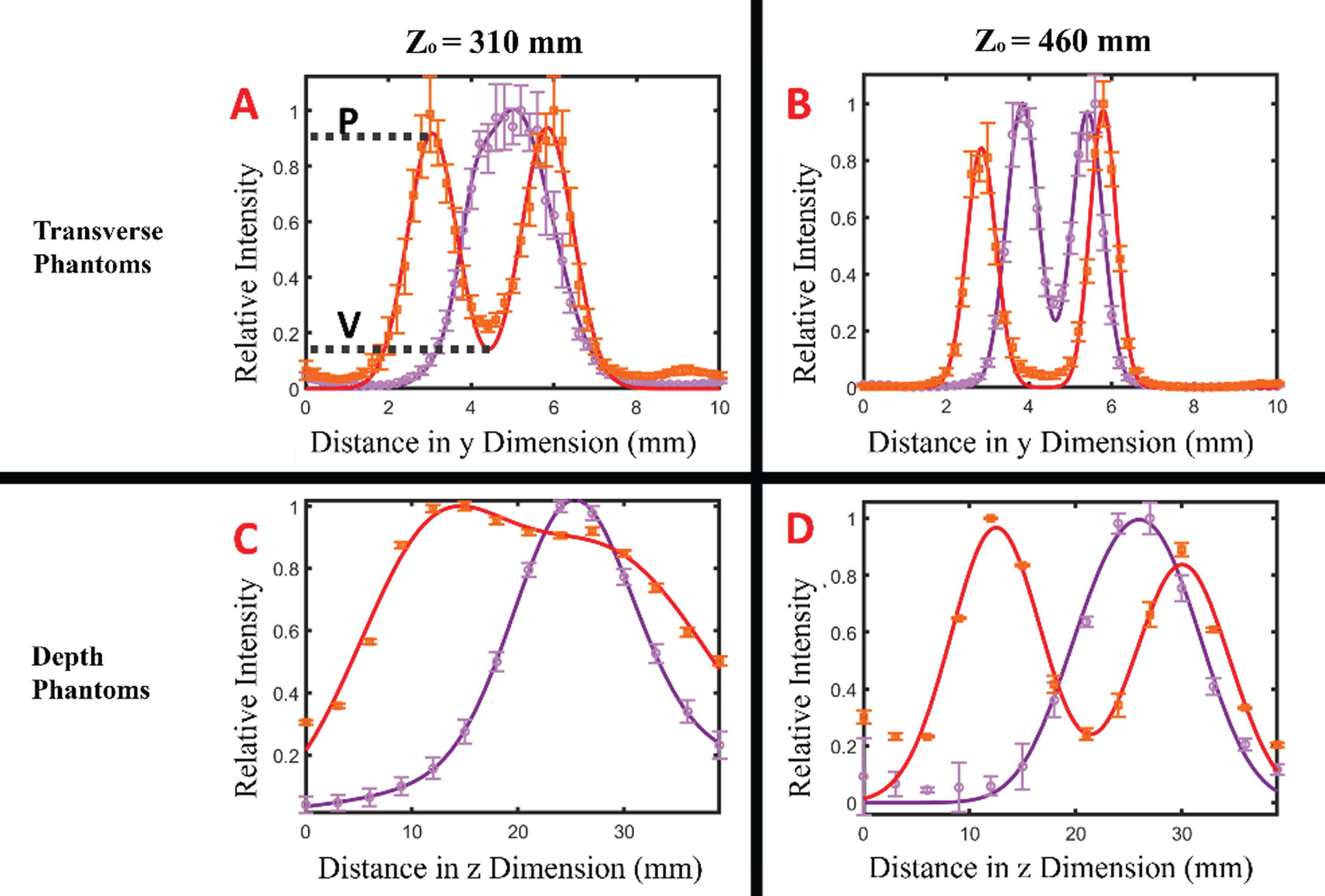
Reconstructed scatter intensity through the transverse and depth resolution phantoms at z_o = 310 mm in plots A) and C) respectively, as well as at z_o = 460 mm in plots B) and D) respectively. They display the contrast (C) between the highly scattering PLA walls, represented by the peaks (P), and the lightly scattering air gaps, represented by the valleys (V), of the scanned phantoms shown in Fig. 3. The data points are the intensity at each voxel along the gap width. Five data sets were collected and averaged for each single plot, with the variation among those 5 plots represented as the error bars. The orange and purple lines correspond to the orange and purple regions of interest seen in Fig. 3. The smooth line of best fit was parameterized as the sum of two Gaussians and optimized using MATLAB’s “Curve Fitting” application. The peaks and valleys from this fit were used in the contrast definition given in Equation (9).

The curves plotted in Fig. 4 are unweighted Gaussian curves of best fit created using MATLAB’s “Curve Fitting” application (MATLAB 2021b, Curve Fitting Toolbox, The MathWorks, Inc., Natick, MA, United States). We assumed that data could be well-represented as the sum of two Gaussians as described in Equation (8). y = a 1 e - ( ( x - b 1 c 1 ) 2 ) + a 2 e - ( ( x - b 2 c 2 ) 2 )(8)

The amplitudes a₁ and a₂, shifts b₁ and b₂, and widths c₁, and c₂ were adjusted to find the curve that most closely fit the data to minimize the root mean squared error (RMSE). The fits generated from this application had average RMSE values of 0.03 and 0.04 for the transverse and depth data respectively, which suggested that the measured point spread function was reasonably well-described as a Gaussian. To determine the system resolution, we used two different approaches: 1) the Gaussian fit widths were used as a description of the full width at half max (FWHM) resolution of the system and 2) the contrast between wall and gap regions of the phantom were used to determine resolvable features based on a Sparrow criterion-like metric. While relating c_1,2 to FWHM resolutions is straightforward, the slightly different heights and fitted widths of the measured signal requires some additional description for evaluating the contrast metric. C = ( P - V ) P(9)

To evaluate the contrast quantitatively, we defined the peak-to-valley ratio stated in Equation (9), consistent with the definitions of Ref. [16], and represented in Fig. 4A. C, P, and V represent the contrast, peak value, and valley value respectively. However, the well-defined peak and valley seen in Fig. 4A is not representative of how distinguished these features are in all data sets. When two Gaussians are the same amplitude, a resolvable valley will have both a positive second derivative, and a first derivative of zero. But when two peaks are not the same height (which was common in the data), there can be an inflection point where the second derivative changes from a negative to a positive value, but the first derivative never reaches zero. There is a continuous downward slope in this case. Figure 4, image C is an example of this. Therefore, we have chosen to define the valley as the intersecting point between the two individual Gaussians and use the intensity value at that location to compare it to the peak value. The peak value is defined as the average peak intensity of the two Gaussians for that measurement. The values of P and V are derived from the fits in Equation (8). If there was a second derivative sign change, from negative to positive, between the two peaks, then this calculation would give a valley value that was less than the average peak height, and therefore a positive, non-zero contrast. This analysis is consistent with the “Modified Sparrow” criterion, which is traditionally applied when evaluating contrast for asymmetric sources [21–23], and was used consistently across all data sets herein. If there was no valley, the contrast value was set to zero and the points were considered unresolvable as defined by the modified Sparrow criterion.

For some cases, the two walls were always resolvable, thus precluding us from determining the minimum resolution in this way. In these cases, we extrapolated our experimental measurements using our Gaussian model and the measurements using Equation (10) V = a 1 e - ( ( x intersect ) 2 2 σ 2 ) + a 2 e - ( ( x intersect - δ ) 2 2 σ 2 )(10) where X intersect = δ 2 + σ 2 δ [ ln ( a 1 / - a 2 ) ] is the location of the minima, δ is the gap separation, σ is the standard deviation of the Gaussian, and a_1,2 are the amplitudes of the Gaussians. The same value of σ is used to describe each Gaussian, to define a singular value of resolution. All parameters were extracted directly from the measured data. σ is inversely proportional to the resolvability of two Gaussians separated by some distance. Therefore, σ can determine the contrast between two Gaussians, which can be used to best fit a set of contrast values that vary due to their relative distance.

The final step of this analysis is to determine the value of σ in Equation (10) such that the calculated value of V, combined with the measured data’s Gaussian fitting parameters, results in contrast values that best fit the measured contrasts of the reconstructed phantom gaps. To accomplish this, we determined the value of σ that minimized the sum-squared error between Equation (10)’s predicted contrast and the measured contrast from the reconstruction. This process assumed that the Gaussian width of each reconstructed wall was constant. The resulting value of σ could then be used to estimate resolution between two gaps of any distance, which could be interpolated or extrapolated to the threshold at which contrast became zero. Examples of this approach can be seen in Fig. 5. The limit at which this occurs is what we will consider minimum system resolution, as this most closely resembles the Sparrow criterion.

OPEN IN VIEWER

Fig. 5

Contrast as a function of gap separation for the transverse and depth phantoms. The data points were calculated using Equation (9) and the Gaussian fit plots seen in Fig. 4, plots B and D. Using Equation (10), a value of sigma was optimized to create contrast trend plots that best fit these data points and is represented by the dashed blue line. The point at which contrast first takes a positive non-zero value is defined as the minimum resolution. Both plots show triangular data points which represent their respective theories for conservative and idealized minimum resolution values (see Table 1).

Figure 6A and 6B show the transverse and the depth resolution as a function of sample location, respectively, both for the predictions of the different resolution theories described above as well as for the experimental measurements of the resolution using different metrics. The “Gaussian Fit FWHM” data points represent the average calculated FWHM values from the Gaussian fitting parameters used to describe the reconstructed measurements. The “Contrast Resolution” data points represent the smallest resolvable gap width, as defined by the threshold at which contrast becomes a positive, non-zero value, for a given sample scanning height according to the sigma optimization of Equation (10).

OPEN IN VIEWER

Fig. 6

Transverse and depth resolution as a function of z_o. In both plots A) and B), the dashed blue line represents the transverse and depth resolution, respectively, as predicted by the Ref. [16] theories. The dashed orange line represents the ideal measurement case of our proposed Geometric theory for transverse resolution, and the dashed green line is the depth resolution prediction based on the Ref. [15] theory. These plots display how the measured resolutions (contrast-based resolution and FWHM based resolution) compare against the various theoretical estimates.

We see that the theoretical predictions of approximately 0.4–2.4 mm transverse resolution and 7–26 mm depth resolution agreed generally with the measured values ranging from 0.6–2 mm and 7–16 mm, respectively (as shown in detail in Table 1). In addition, both theory and experiment showed improved resolution for larger values of z_o throughout the considered field of view.

We also considered how the system geometry and varying spatial resolution impacted the system’s momentum transfer (q) resolution. Figure 7 shows the combined XRD coherent and Compton scatter form factor to give a normalized total angular-scatter intensity plot for PLA obtained through measurement in a commercial diffractometer (red line) and in our system (blue line with error bars) for each value of z_o. The diffractometer used is a Bruker AXS D2 Phaser (Bruker –Billerica, MA. Manufactured 2013), which has been converted to momentum transfer space based on the copper k-alpha line at approximately 8.04 keV. Due to the relatively small angle of the scatter being considered and the relatively low energy of the X-rays (compared to an electron’s rest-mass), these plots are a good approximation of the coherent scatter form factor for a similar measurement. The data points and associated error bars measured in our system arise from averaging and considering the standard deviation across the angular scatter intensity of 20 reconstructed voxels associated with the PLA walls of the phantom. Plots A, B, C, and D of Fig. 7 represent the sample scanning locations of z_o = 310, 360, 410, and 460 mm respectively. In each plot the peak around q = 0.1 Å^–1 generally aligns with the ground truth peak and the shapes are consistent with the ground truth. However, the momentum transfer resolution degrades as z_o increases (the 310, 360, 410, and 460 mm sample plane measurements show a RMSE of 0.16, 0.14, 0.21. and 0.28 normalized total scattering intensity, respectively), thus indicating an important potential tradeoff between spatial resolution and momentum transfer resolution. This tradeoff stems from the fact that the momentum transfer resolution depends on the angular uncertainty of the measurement, which comes both from localization of the scatter (i.e., spatial resolution) and localization of the measured X-ray (i.e., coded detector resolution). These quantities vary in conflict with one another as a function of z_o, thus suggesting an optimal value for a given sample size and composition.

OPEN IN VIEWER

Fig. 7

A), B), C), D), Average combined XRD coherent and Compton scatter form factors to give a normalized total angular-scatter intensity for the PLA walls of the depth resolution phantom measurements at z_o = 310, 360, 410, and 460 mm, respectively. Error bars were plotted as one standard deviation derived from 20 different pixels used to create the average coherent scatter form factor in the plots. In addition, the plotted orange line represents a ground truth PLA total scatter signal based on measurements made with a commercial diffractometer.

A useful imaging modality should have quantities such as spatial resolution that are measurable, predictable, and well understood. The existing literature on CA-XRDI has provided an initial basis for characterizing such systems but has neither been directly interpretable and/or applicable to a broad set of circumstances nor consistent among its predictions.

This work reviews the existing resolution models for CA-XRDI systems and proposes a new ‘geometric’ model that is specifically relevant to limited angle coded aperture scatter systems. In addition, we provided experimental validation of first-principle theories across a broad range of the relevant parameter space using custom, 3D printed phantoms. By reconstructing a 4D data-cube consisting of the XRD form factor throughout a 3D volumetric space, we showed that the transverse and depth spatial resolutions are bounded by the various theories considered.

In particular, we found that the Ref. [16] theory was an overly-conservative estimate for our transverse CA-XRDI resolution due to its assumptions about isotropic, unstructured scatter being the only source of spatial information. Conversely, our Geometric theory can be described as the idealized best-case scenario for resolution due to its assumption about perfect scatter sources and detector responses. Similarly for the case of depth resolution, the Hassan theory for depth resolution was likely a conservative estimate due to it defining resolvable signal as a full code period difference due to magnification at the detector. The MacCabe theory, on the other hand, more reasonably predicted a better resolution and matched our finding because, for sufficiently fine pixel sampling at the detector, shifts of less than one whole period shift could be reasonably detected.

In general, we found that the experimentally observed resolution values sat between the more and less conservative resolution estimation theories against which we compared our findings. The FWHM data points were, conceptually, closer to PSF-type characterizations of resolution and, therefore, tended to align well with the more idealized resolution limit for transverse and depth measurements (Geometric and MacCabe theories, respectively). The contrast-based resolution metric akin to the Sparrow criterion (or “Contrast Resolution” in Fig. 6) tended to provide a larger estimate of resolution more consistent with the more conservative Hassan theories.

While the resolution theories provide a reasonable estimate for the measured spatial resolution, we note that there are several effects that were not considered by the theories that may impact the results. First, residual model mismatch between the forward model and experimental data can result in reconstruction artifacts and reduced resolution. For example, the current reconstruction calculation does not correct phenomena such as self-attenuation or multiple scattering, which become more apparent as objects become thicker and more attenuating to the incident X-rays. Second, it should be noted that the nature of an iterative reconstruction process tends to accentuate high frequency information, such as that seen at a boundary between a wall and air gap. This can result in increased noise as well as artificially sharpened peaks if too many iterations are used. Finally, the theories discussed here do not explicitly consider the finite size of the focal spot, focal spot drift, source and detector spectral characteristics, or the finite thickness of the coded aperture, which can provide additional fundamental limitations to the spatial resolution. The construction of higher-resolution, faster 3D XRDI systems operating on increasingly complex samples will benefit from the results presented here but will also require a deeper evaluation of the nuanced aspects of the system that determine the spatial resolution.