Decomposition iteration strategy for low-dose CT denoising

Abstract

In the medical field, computed tomography (CT) is a commonly used examination method, but the radiation generated increases the risk of illness in patients. Therefore, low-dose scanning schemes have attracted attention, in which noise reduction is essential. We propose a purposeful and interpretable decomposition iterative network (DISN) for low-dose CT denoising. This method aims to make the network design interpretable and improve the fidelity of details, rather than blindly designing or using deep CNN architecture. The experiment is trained and tested on multiple data sets. The results show that the DISN method can restore the low-dose CT image structure and improve the diagnostic performance when the image details are limited. Compared with other algorithms, DISN has better quantitative and visual performance, and has potential clinical application prospects.

Keywords

LDCT decomposition image denoising iteration CNN

1 Introduction

Larger doses of radiation can cause harm to the human body. When patients absorb more than the normal dose of X-ray radiation, metabolic abnormalities will be caused, and even cancer and other diseases [1]. With the widespread use of medical CT, the potential risk of radiation dose in patients cannot be ignored. However, dose reduction leads to decreased photon density and increased noise in the scan, necessitating the development of denoising methods to ensure image quality and retain the clinical information contained within [2]. Therefore, reducing the scan dose while obtaining high-quality LDCT images is a challenging task that requires the use of advanced methods and techniques.

To improve the quality of CT images, researchers have proposed a variety of image denoising methods that can be categorized into three types: projection domain processing before reconstruction, iterative reconstruction processing during reconstruction, and post-processing after reconstruction. Projection domain methods include bilateral filtering [3] and structural adaptive filtering [4], but these methods may lead to image edge blurring and detail structure loss. The method based on iterative reconstruction (IR) first initializes the image and then updates the initial value through the forward projection operation to gradually approach the real target image. The commonly used methods include total variation (TV) and its variants [5, 6], and dictionary learning [7, 8]. Both methods require the use of raw projection domain data, which is hard to obtain in practical studies, increasing the research difficulty. Compared with other techniques, image post-processing techniques can be used to process LDCT images directly and can be easily combined with existing clinical procedures. Traditional image post-processing algorithms include improved BM3D method [9 –12], non-local means method [13, 14], partial differential equation (PDE) method [15 –17], dictionary learning [18], wavelet transform [19], etc. Although these operators can reduce noise to some extent, they often result in excessively smoothed or erroneous LDCT images after denoising. This is because these traditional methods may not fully consider the complex and diverse noise characteristics of LDCT images, resulting in compromised image details and important pathological information.

Using the nonlinear mapping ability of deep convolutional neural networks, some methods based on deep learning have obtained better results in reducing LDCT image noise. Chen et al. [20] proposed a neural network with an encoder-decoder structure (REDCNN) for LDCT images. Fan et al. [21] designed a quadratic auto encoder (Q-AE) network using secondary neurons and auto encoders, which effectively improved the denoising effect of LDCT images. Kang et al. [22] proposed a method for the study of deep convolutional neural networks for the reconstruction of LDCT images using directional wavelets. However, these methods still have the problem of processing noise while maintaining image details. Liang et al. [23] proposed the EDCNN algorithm in 2017, whose core idea is to use convolutional neural networks to extract edge information in images and fuse this information together through dense connections to achieve efficient and accurate LDCT image denoising. Jiang et al. [24] proposed FSNet using a novel hybrid convolutional and adaptive aggregation approach for LDCT image denoising by learning frequency separation networks, and achieved better performance. The method proposed by Gholizadeh-Ansari et al. [25] uses a CNN architecture that includes perceptual loss and edge detection layers. The perceptive loss layer used the pre-trained VGG-16 network to calculate the feature similarity between the reconstructed image and the corresponding NDCT image as a measure of image quality. The edge detection layer is designed to preserve the edges and important structures in the reconstructed image and prevent over-smoothing. Li et al. [26] introduced a novel LDCT denoising algorithm which is based on deep convolutional neural network and multi-scale feature fusion, which can be used to effectively remove noise from LDCT images while retaining more detailed information. Generative adversarial network (GAN) has great application potential and can bring more accurate and efficient solutions for LDCT image processing. Wolterink et al. [27] proposed a novel LDCT image denoising algorithm based on GAN. The algorithm relies on the generative power of GAN to produce realistic high-quality LDCT images by learning the mapping relationship between LDCT images and NDCT images through adversarial learning. Yang et al. [28] designed a GAN algorithm based on Wasserstein distance and perceptual loss for LDCT image denoising. The algorithm employs GAN to achieve high-quality LDCT image reconstruction, which effectively reduces the noise level of LDCT images. Geng et al. [29] proposed a medical image denoising algorithm using content-noise complementary learning under GAN networks. The algorithm achieves the operation of processing both noise and content information under the same network structure through two modules: the noise module and the content module, thus improving the effectiveness of medical image denoising. Han et al. [30] proposed an LDCT image denoising network using a dual encoder single decoder. The network learns the feature representations of LDCT images and high-dose CT images separately by using a dual encoder model, and combines them to reconstruct low-dose CT images. Marcos et al. [31] proposed a GAN network with the introduction of the SE module and CBAM module. The enhanced attention module is used to preserve the structural details of LDCT images. However, the training process of GAN is usually unstable and may produce artifacts inconsistent with NDCT. The proposal of the multi-domain network also provides a new possibility for LDCT image denoising. Lyu et al. [32] proposed a two-domain network, U-DuDoNet, to add artifacts in the sinogram and image domains using U-Net to directly model the artifact generation process to remove CT image noise. Yin et al. [33] presented a region progressive three-dimensional residual convolution network DP-ResNet, which designs networks in the sinusoidal domain, filtered back projection domain and image domain to achieve denoising. In recent years, researchers have tried to apply transformer to medical image denoising. Wang et al. [34] proposed a Transformer-based LDCT image denoising method CTformer. Different from the traditional CNN-based method, CTformer adopts pure Transformer structure to avoid convolution operation, making the model more efficient and easy to optimize.

Although the CNN-based low-dose CT noise reduction method has achieved satisfactory results, due to its abstract mapping function fitting process and lack of intuitive interpretation, two problems are proposed: (1) How to use the physical model to make the designed LDCT noise reduction network interpretable. (2) How to improve the model’s ability to maintain low-frequency smoothing and reconstruct high-frequency details. Therefore, for the denoising task of LDCT images, it is necessary to explore a new strategy to better utilize the unique characteristics of physical models and CT images and combine physical models with deep learning.

In the image denoising task, it has undergone an evolution from model-driven to data-driven. The advantage of model-driven is that it is easier to explain and can denoise single samples, but its shortcomings are also obvious, that is, it relies heavily on prior estimation. If the prior estimation is inaccurate, there will be obvious problems. At the same time, the algorithm design is difficult and the robustness is poor. The biggest problem of data-driven is unexplainable, which is actually to fit an end-to-end mapping through a large amount of data, but this mapping is expressed as a neural network. The quality of data-driven results depends heavily on the rationality of network design. If we can combine data-driven and model-driven, we can solve the inherent unexplainable problems in deep learning, and make full use of data features to make the whole model more reasonable and have better generalization ability. Therefore, a new strategy needs to be explored in image denoising tasks to better combine data-driven and model-driven. To solve these problems, we fully consider the physical model of the task when designing the network, and build a reasonable network according to the corresponding relationship of the physical model. We propose a purposeful and interpretable decomposition iteration strategy network (DISN) for LDCT denoising. The method shown in this paper resulted in good noise reduction on the 2016 NIH AAPM Mayo Clinic LDCT dataset [35], the piglet dataset [36] and the clinical dataset. The main salient points in this paper are the following:

DISN based on decomposition iteration is a new architecture for the interpretability of LDCT denoising networks.

Since there is a certain correlation between noise/artifact and inherent information, in order to preserve the edge/texture in the iterative process, we use the Hessian matrix to realize the frequency distribution of the image and decompose the LDCT image into low and high frequency, which effectively improves the ability of the model to maintain low frequency smoothing and reconstruct high frequency details.

For the decomposed high frequency and low frequency information, the corresponding network is designed respectively, and in order to better process the obtained low frequency content features and the processed high frequency texture features, a fusion network is also designed.

To verify the capability of the LDCT image denoising network, several data sets were used, including the 2016 NIH AAPM Mayo Clinic LDCT dataset, piglet data with different radiation doses, and clinical data. After verification, the proposed DISN has good noise suppression and edge detail protection ability.

The remainder of this article is constructed as shown below. The second part reviews the knowledge related to LDCT image noise reduction, and introduces the DISN framework in detail, including the use of the Hessian matrix to decompose the image, the design of low frequency network and high frequency network after decomposition, the network design of high frequency and low frequency information fusion. The third part gives the specific experimental design and relative comparison experiment. Finally, we will discuss the related issues of LDCT image noise reduction in the fourth part, and make a summary of this paper.

2 Methods

2.1 Noise reduction model

The LDCT image denoising model can be represented as a reflection projection process from LDCT image X to NDCT image Y: $X = T (Y)$ (1)

T denotes the nonlinear degradation process from the NDCT image Y to the corresponding threshold LDCT image X. The denoising process can be transformed into the mapping f: $\underset{f}{arg min} {∥ f (X) - Y ∥}_{2}^{2}$ (2) where f is the optimal approximation function obtained through deep learning.

2.2 Decomposition iterative framework

In LDCT image denoising tasks, it is usually assumed to be a linear model, which can be expressed as: $X = B + N$ (3)

In this model, X denotes a noisy LDCT image, B denotes a clean CT image to be recovered, and N denotes noise. We can develop state-of-the-art denoising networks by learning the resulting mapping from noisy images to potentially clean images.

However, as CT images can be made up of low and high frequency information, in this work we make use of an alternative composition of images, whose model can be expressed as: $X = H + L$ (4) where H is the high frequency information of the LDCT image and L is the low frequency information of the LDCT image.

Decomposition iteration idea is integrated into the LDCT image denoising process to learn in the DISN process rather than a simple linear combination of the noisy image and the denoised clean image. DISN is an iterative framework with n iterations summarized in the following steps:

In considering the forward problem, we assume the existence of a mapping such that: $D (I) = (L, H)$ (5)

That is, the input to the network is the low-dose CT image I to be processed, and the input image is first decomposed into low and high frequency information. However, in this process, we iterate by using the residuals, so there is: $D (Δ I_{n}) = (Δ L_{n}, Δ H_{n})$ (6)

In the initial condition, ΔI₀ = I. For the current residual image ΔI_n, the residual components ΔL_n, ΔH_n can be decomposed using the image decomposition.

In considering this task from an inverse problem perspective, this paper argues that there exists a mapping such that: $F (Δ L_{n}, Δ H_{n}) = Δ I_{n}$ (7)

The input of the network is the processed low and high frequency information, and the output of the network is the image after noise reduction in the DISN process, and F (·) is the network that fuses low-frequency information and high-frequency information. $L_{n} = L_{n - 1} + L (Δ L_{n})$ (8) $H_{n} = H_{n - 1} + H (Δ H_{n})$ (9)

Because of the large difference between low and high-frequency information, we designed a sub-network, L (·) for the low-frequency network dealing with low frequency information and H (·) for the high frequency network dealing with high-frequency information, respectively. Then refine the low and the high frequency information L_n, H_n by adding these residual components. $Δ Z_{n} = F_{n} - F_{n - 1}$ (10)

With infinite iterations, n→ ∞ when ΔI_n → 0 such that the LDCT images converge to the NDCT images. Based on the whole decomposition iteration strategy, we propose a purposeful and interpretable decomposition iteration network (DISN), which is a new, specific LDCT noise reduction method aiming to improve the detail fidelity instead of blindly designing or using a deep CNN architecture. The whole process is shown in Fig. 1.

Fig. 1

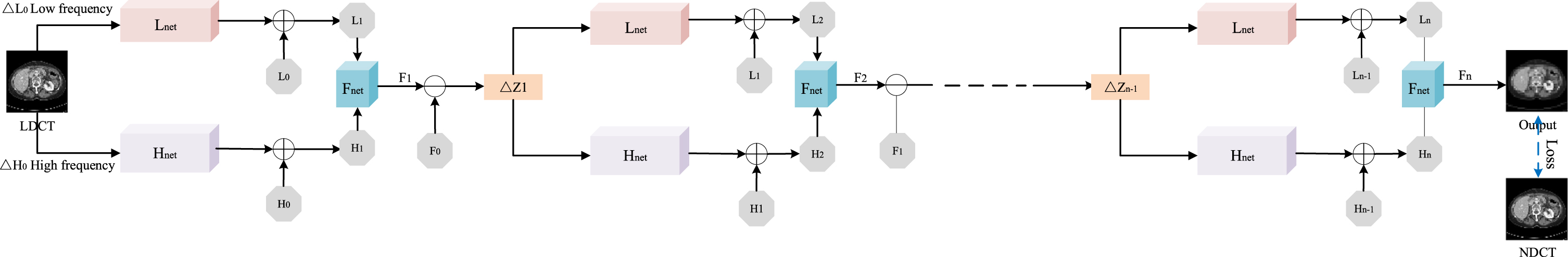
The proposed decomposition iterative strategy (DISN) pipeline for LDCT denoising.

This study combines a physical model and explores a decomposition iteration strategy suitable for low-dose CT image denoising. In this study, the image denoising is carried out in an iterative manner, and the image is decomposed into high-frequency and low-frequency parts, and the multi-stage denoising effect is realized by image difference. First, the low-dose CT image is decomposed into a high-frequency part and a low-frequency part using the Hessian matrix. The high frequency part mainly contains the details of the image, and the low frequency part contains the overall structure and background information. Then, the deep learning network is used to denoise the high-frequency part to restore the details and remove the noise. Using deep learning network to the low frequency part. It is processed separately to improve the clarity of the overall structure and the accuracy of the background information. Finally, the noise reduction processed.

2.3 Attention mechanism

In the CT image decomposition stage, we use the Hessian Filter method. the Hessian matrix, a filter based on the second-order gradient information of an image, was early applied to tasks such as edge detection and corner point detection in computer vision. Since Hessian Filter is very sensitive to noise, this method is also widely used in LDCT image denoising, usually by extracting the high-frequency part of the image (i.e., noise), then filtering it using Hessian Filter to eliminate the high-frequency noise, and finally obtaining the low-frequency part and reconstructing it with the original image. The Hessian matrix is determined by the image’s partial derivatives in the horizontal and vertical directions are determined as: $H = [\begin{matrix} I_{xx} & I_{xy} \\ I_{yx} & I_{yy} \end{matrix}]$ (11)

The Hessian matrix is represented in Eq.(11). as a symmetric matrix of second-order partial derivatives, where I_xx, I_yy, and I_xy(I_yx) denote the horizontal, vertical, and mixed second-order partial derivatives of x. The maximum eigenvalue of the Hessian matrix can be used to describe the intensity of the edges of image structure and has a good measurement capability in terms of residual images, which can effectively improve the image detail fidelity. It should be noted that the calculation of the Hessian matrix requires needs to use its second derivative, which can be obtained by applying some specific filters. $I_{xx} = [\begin{matrix} 0 & 0 & 0 \\ 1 & - 2 & 1 \\ 0 & 0 & 0 \end{matrix}] I_{yy} = I_{xx}^{T}, I_{xy} = I_{yx} = [\begin{matrix} 1 & 0 & - 1 \\ 0 & 0 & 0 \\ - 1 & 0 & 1 \end{matrix}]$ (12)

Characterize image detail fidelity using the maximum eigenvalue of the Hessian matrix, which is usually calculated using the eigenvalue decomposition. The eigenvalue and the corresponding eigenvector of the Hessian matrix represent the magnitude and direction of the curvature of the point in a given direction, respectively. The Hessian matrix in Eq.(12). is a real symmetric matrix, so the relationship between the eigenvalues (λ1> λ2), trace tr(H(x)) and determinant |H(x)| can be deduced using the knowledge of linear algebra. A real symmetric matrix has many important properties, among which are that all its eigenvalues are real and the eigenvectors are orthogonal. These properties make it easier to perform eigenvalue decomposition to obtain the eigenvalues and eigenvectors of a Hessian matrix. $| λ E - H | = 0, | λ [\begin{matrix} E - I_{xx} & E - I_{xy} \\ E - I_{yx} & E - I_{yy} \end{matrix}] | = 0$ (13)

For a pixel in an image, its Hessian matrix is 2×2, so there must be two eigenvalues. $tr (H) = I_{xx} + I_{yy} = λ_{1} + λ_{2}, | H | = I_{xx} I_{yy} - I_{xy} I_{yx} = λ_{1} λ_{2}$ (14)

Since only a pixel-by-pixel gradient is required, this Hessian filtering process can be accelerated using the specific convolution in (12).

More generally, λ is an algebraic combination of the second-order gradients of x and λ ∝ ∑_i=-1,0,1 ∇ xⁱ, where ∇ denotes the gradient extractor through (12).

The Hessian filter takes the high frequency information portion of the original image and then subtracts it from the original LDCT image to obtain the low frequency information of the image.

2.4 DISN architecture

To fully extract the features in LDCT images, the designed DISN consists of three sub-networks, namely, low frequency network L_net, which processes low frequency information, high frequency network H_net, which processes high frequency information, and fusion network F_net. The DISN is an iterative framework in which each sub-network shares parameters at different stages. In this section, we introduce the network architectures of the low frequency network, the high frequency network, and the fusion network.

2.4.1 Low frequency network architecture

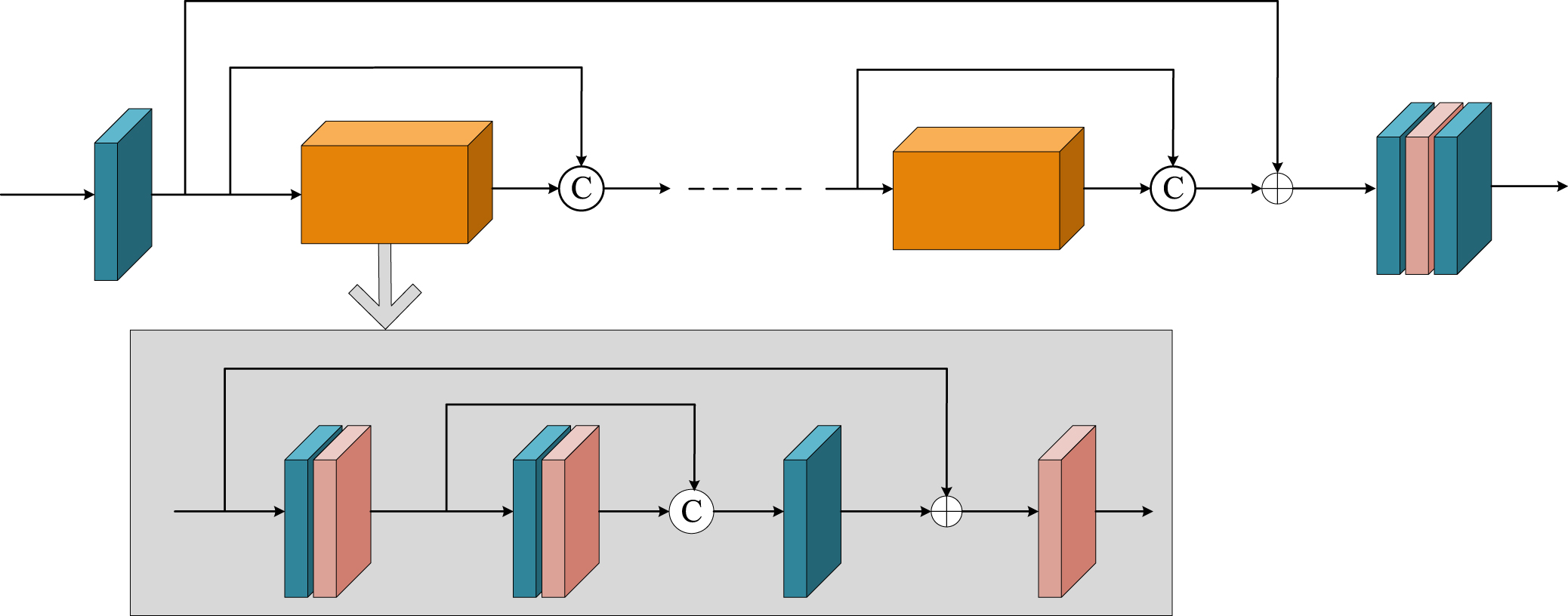
We designed the low-frequency network architecture to adequately train to extract low-frequency content features. The architecture consists of multichannel residual blocks (MCRB) and multiscale residual blocks (MSRB). As shown in Fig. 2, the number of sub-blocks consisting of multichannel residual blocks and multiscale residual blocks we set is 3. The multiscale residual block first acquires multiscale features using Pooling operations with different kernel sizes and step sizes, and then fuses and feeds all scales into the Conv + PReLU and Conv + PReLU + Conv layers with the original input signal to learn the residuals. MSRB can learn features at different scales and fuse all different features to learn the main features. In addition, we use a multi-channel residual block to process the important low-frequency information, which consists of multiple channel attention modules and residual blocks. The shallow information is extracted first, and then the information is channelized by three channel attention modules to obtain the important low-frequency information. The information obtained from all channel attention modules is fused and fed into the Conv + PReLU + Conv layer with the original input signal to learn the residuals as a way to learn the processing results of low-frequency information.

Fig. 2

(a) Low frequency network architecture (b) MSRB module (c) MCRB module.

2.4.2 High frequency network architecture

In order to improve the training effect and fully extract the high-frequency content features, we deeply studied the design of the network architecture. Finally, we successfully constructed a unique high-frequency network architecture. The core of the architecture is a cascaded multi-block network composed of three residual structures, represented by a gray box, as shown in Fig. 3. First, the entire network performs preliminary processing of the input data through the Conv layer, with the aim of extracting initial information. This layer plays an important role in the network, which can quickly and effectively filter out useful features from the original data. Then, the network enters the first residual structure block. This structural block is composed of several different layers, which are carefully designed to capture and transmit feature information. The design of this residual structure is inspired by the residual learning idea in deep learning, which optimizes network training through skip connections. Then, the network will experience another cycle of residual structure blocks. In this process, the network further improves its ability to extract high-frequency information by learning residuals. This design allows the network to better understand and extract high-frequency details in the input signal. Finally, after multiple residual structure processing, the network performs the final extraction process through the Conv + PReLU + Conv layer. The design goal of this layer is to accurately extract and optimize high-frequency information. In this way, the network completes the task of fully extracting high-frequency content features from the input signal. In general, our designed high-frequency network architecture can effectively extract and optimize high-frequency content features through a multi-block cascaded residual structure and an accurate Conv layer. This design idea has achieved remarkable results in the process of network training, which provides higher accuracy and efficiency for our model in dealing with high-frequency information.

Fig. 3

High frequency network architecture.

2.4.3 Fusion network architecture

Most of the existing fusion methods treat channel and pixel features in the same way when dealing with image features. However, this method may not fully consider the importance of different parts of the image and different types of information. Therefore, we design a unique fusion network (as shown in Fig. 4), which is mainly composed of local residual learning, channel attention module and pixel attention module. The local residual learning part allows the network to establish multiple local residual connections, which enables the network to better focus on the important information in the image and ignore some less important information. In this way, the network can focus more on dealing with effective information that has a greater impact on the results. The introduction of the channel attention module and the pixel attention module provides the network with additional flexibility, enabling it to adjust the processing method according to different tasks and input images. These modules can extend the representation ability of Convolutional Neural Network, making the network more flexible and effective in processing different types of image information.

Fig. 4

Fusion network architecture.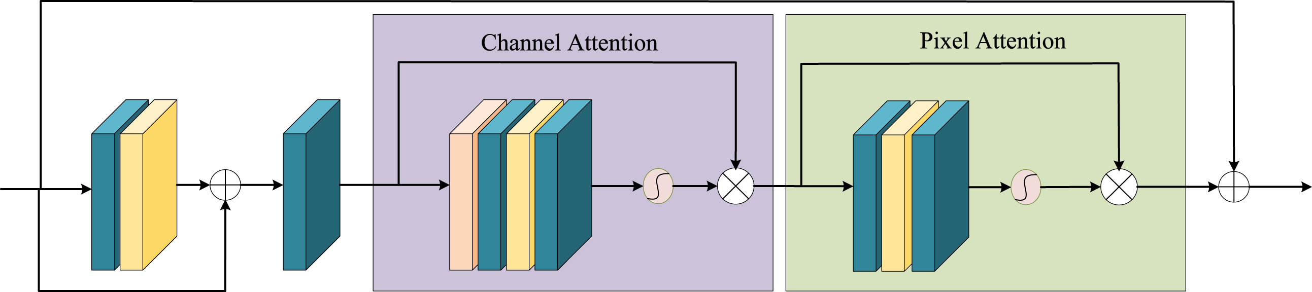

f_{1} = conv (ReLU (f_{0}))

(15)

f_{2} = conv (f_{0} + f_{1})

(16)

f_{3} = f_{channel} = f_{2} \otimes sigmoid (Averagepool (conv (ReLu (cnov (f_{2})))))

(17)

f_{fusion} = f_{0} + f_{3} \otimes sigmoid (conv (ReLU (conv (f_{3}))))

(18)

2.5 Learning objectives

To train a DISN network for LDCT image denoising, we can apply supervision on the NDCT image and the denoised image LDCT after N iterations. The L1 loss function, also known as mean absolute error (MAE), is a measurement method that measures the difference between two vectors. It calculates the average absolute value of the difference between the predicted value and the true value. The L1 loss function is more robust to outliers. When the L1 loss function is used, the predicted results of the model tend to be closer to the median of the true value. Therefore, we use L1 loss to train the final DISN. $L (P) = \frac{1}{N} | | NDCT - DISN (LDCT) | |_{1}$ (19)

3 Experiment configuration and results

In this section, we test performance and generality of proposed denoising method by validating it on different datasets. Specifically, we choose the Mayo dataset, the Piglet dataset and the clinical dataset for our experiments. As can be seen in Fig. 5, different types of medical images have different noise characteristics. The CT images in the Mayo dataset are scanned using a thin-layer technique with high voxel resolution, and the Mayo low-dose CT dataset has a lower scan dose and is louder relative to noise compared to conventional CT scans. The Piglet dataset contains CT image data from five piglets born less than 24 hours after birth, with different application scenarios and the same type of noise compared to the human CT dataset. The noise of the clinical dataset is more expressive compared to the simulated dataset noise. During the training process, we utilized a data augmentation strategy of randomly cropping patches. Specifically, we set the patch size to 60×60 with a sliding interval of 60 pixels for both the input batch of LDCT images and the corresponding target batch of NDCT images. We experimented with several parameter combinations and ultimately chose the following parameters: an Adam optimizer was used to optimize the network weights during training, with an initial learning rate α of 0.0002, a batch size of 6, and two exponential decay factors β1 = 0.5 and β2 = 0.999. We performed 500 training iterations to converge the model with 3 epochs. Our network model was developed using the PyTorch framework and implemented on an Intel (R) Core (TM) i9-10900X CPU @3,10 GHz; 32 GB RAW, GPU NVIDIA RTX A5000. Although patch-based training was employed, the proposed network can handle images of any size. All test images are directly fed into the network without decomposition.

Fig. 5

LDCT images of different data sets.

We used five metrics to compare and analyze the post-experimental images. Structural similarity based on the structural difference (SSIM) [37], peak signal-to-noise ratio (PSNR) based on pixel grayscale difference, gradient similarity deviation (GMSD) [38] based on gradient change, feature similarity metric measure (FSIM) [39] based on feature difference, and multiscale pixel domain implementation metric (VIFS) [40] based on visual perception is used. SSIM calculates the product of luminance similarity, contrast similarity, and structural similarity, and then predicts the local image quality at a certain location. The higher the SSIM, the higher the similarity of the denoised image to the reference image. The FSIM combines the similarity of the phase coherence map and the gradient magnitude map between the reference image and the processed image. VIFS is to extract information of different frequencies on multiple scales of the image, and then use this information to calculate the similarity between images, to obtain the similarity evaluation index. As with SSIM, the higher the FSIM and VIFS values, the better the image quality. The GMSD represents the similarity between the reference image and the processed image in terms of the gradient magnitude map at the pixel level, and the GMSD score is lower for good processing. The implementation of these metric methods procedures is based on their official code, and their parameters are set according to the recommendations of the documentation.

3.1 Mayo experiments

3.1.1 Experimental details

The dataset used in this section is the Mayo CT dataset. Paired NDCT images and corresponding 25% -dose CT (LDCT) images from 10 patients were taken, where quarter-dose data were simulated by adding Poisson noise to the full-dose projection data. The image size is 512×512 and the data format is DICOM. Therefore, the network model uses LDCT images as input and NDCT images as supervised images. The dataset was segmented before training, and the CT images of 9 patients (812 pairs) were randomly selected as the training set, and the images of the remaining 1 patient (83 pairs) were used as the test set. By dividing the data in this way, we can ensure that there is enough data in the training set for network learning, but also be able to evaluate and validate the model’s abilities to generalize on a separate test set. In the context of visual effectiveness and quantifiable assessment, we compared the residual-based REDCNN [20], edge-based EDCNN [23], quadratic self-encoder QAE [21], transformer-based CTformer [34], physical model-based CNCL [29], GAN network-based WGAN_VGG [28], and multi-scale architecture of MSFLNet [26]. For a fair comparison, all methods use the configurations recommended in the corresponding papers.

3.1.2 Qualitative assessment

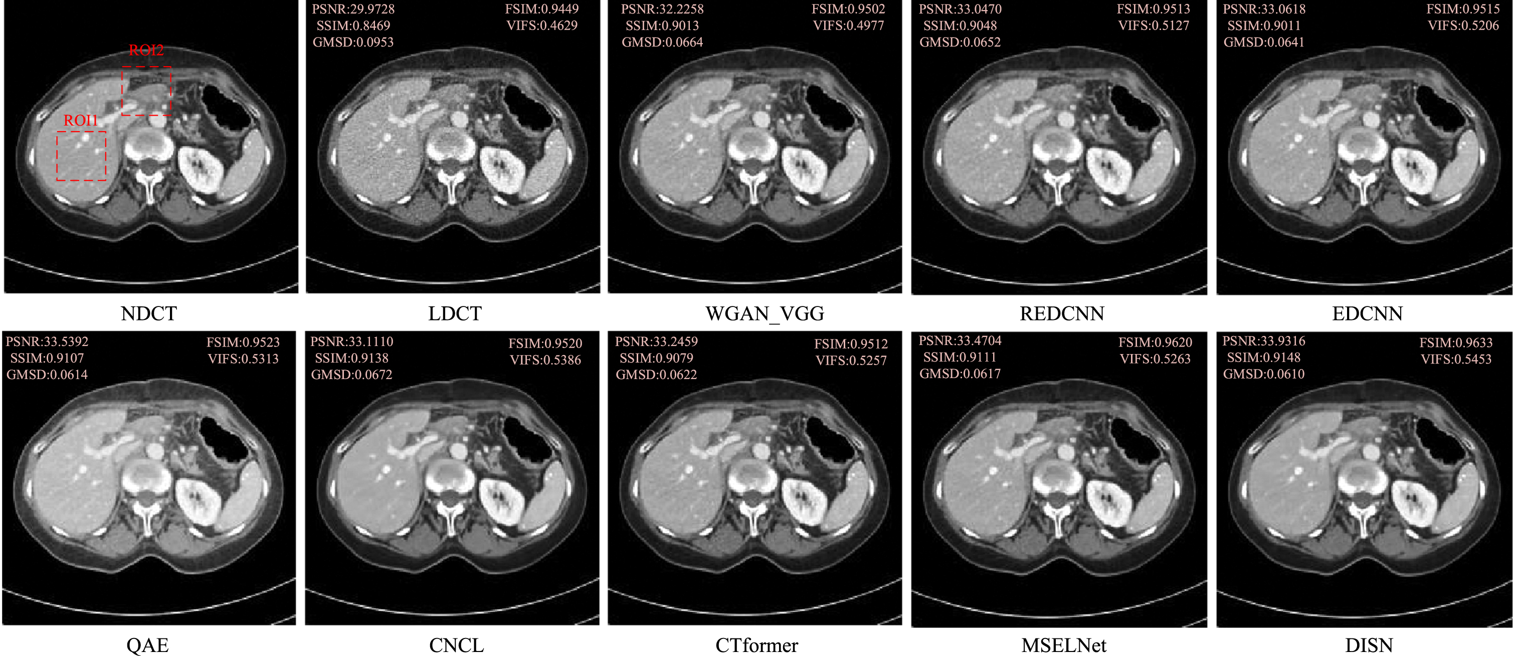
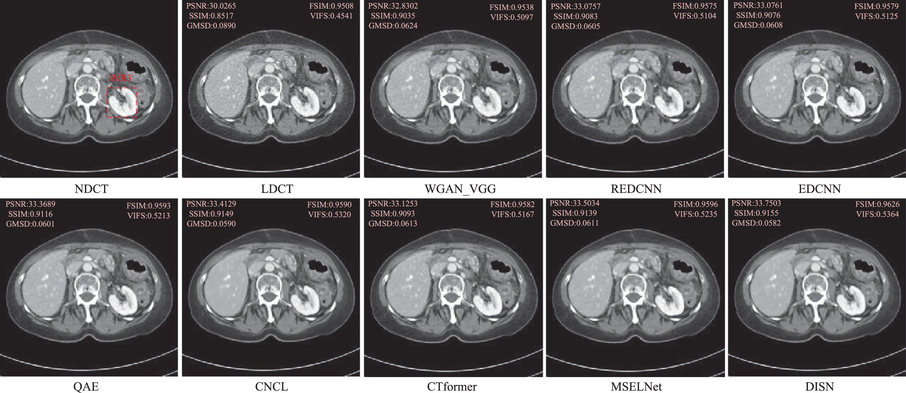
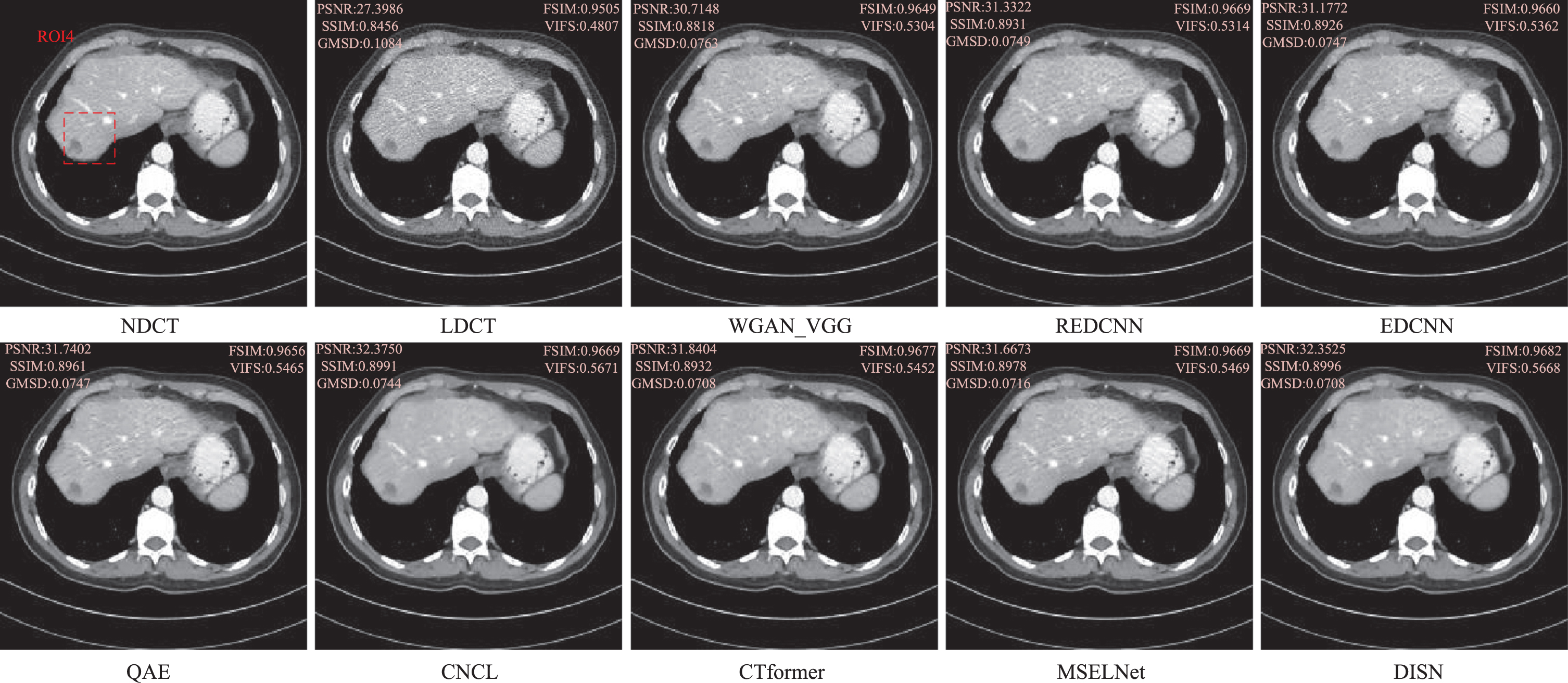
In the qualitative evaluation, these methods showed different degrees of noise suppression ability. As can be seen in Figs. 6∼8, we selected three representative CT images from the test set, and all CT images in the axial view are shown in the [–160HU, 240HU] window to visually analyze several representative denoising results, Fig. 6 and 7 are CT images of the abdomen, and Fig. 8 is a CT image with a lesion. To show the noise reduction effect more clearly, we zoomed in on the region of interest (ROI), as shown in Fig. 9. Although REDCNN has a certain effect on noise suppression, the processing results over-smoothed the image details. EDCNN pays attention to preserving image edge information, effectively avoiding the information loss caused by image edge blur, but in some complex edge regions, the denoising effect is limited to a certain extent, resulting in sharpening and false edges in the restored image. Although QAE can restore low-dose CT images better, it relies too much on high-frequency information, which leads to a bit of blurring in detail processing after noise reduction, and the whole image looks a bit smooth and introduces artifacts. CT former removes most of the global features and local relationship information of LDCT images by learning CNCL effectively removes the noise and artifacts in LDCT images, but there are problems of image smoothing and loss of details, etc. MSFLNet can learn the high frequency detail information of LDCT images through multi-level feature extraction and fusion, and has better restoration ability, but compared with the image clarity, some details of processing are still lacking. Our DISN has the best noise reduction effect compared to these algorithms, and achieves better results in artifact removal and tissue detail protection. This experimental result shows that our decomposition-based iterative denoising strategy has a strong noise and artifact removal capability. In conclusion, DISN has excellent capabilities in removing noise and artifacts and restoring image details and textures.

Fig. 6

The noise reduction results of sample 1 in AAPM data set are visually displayed.

Fig. 7

The noise reduction results of sample 2 in AAPM data set are visually displayed.

Fig. 8

The noise reduction results of sample 3 in AAPM data set are visually displayed.

Fig. 9

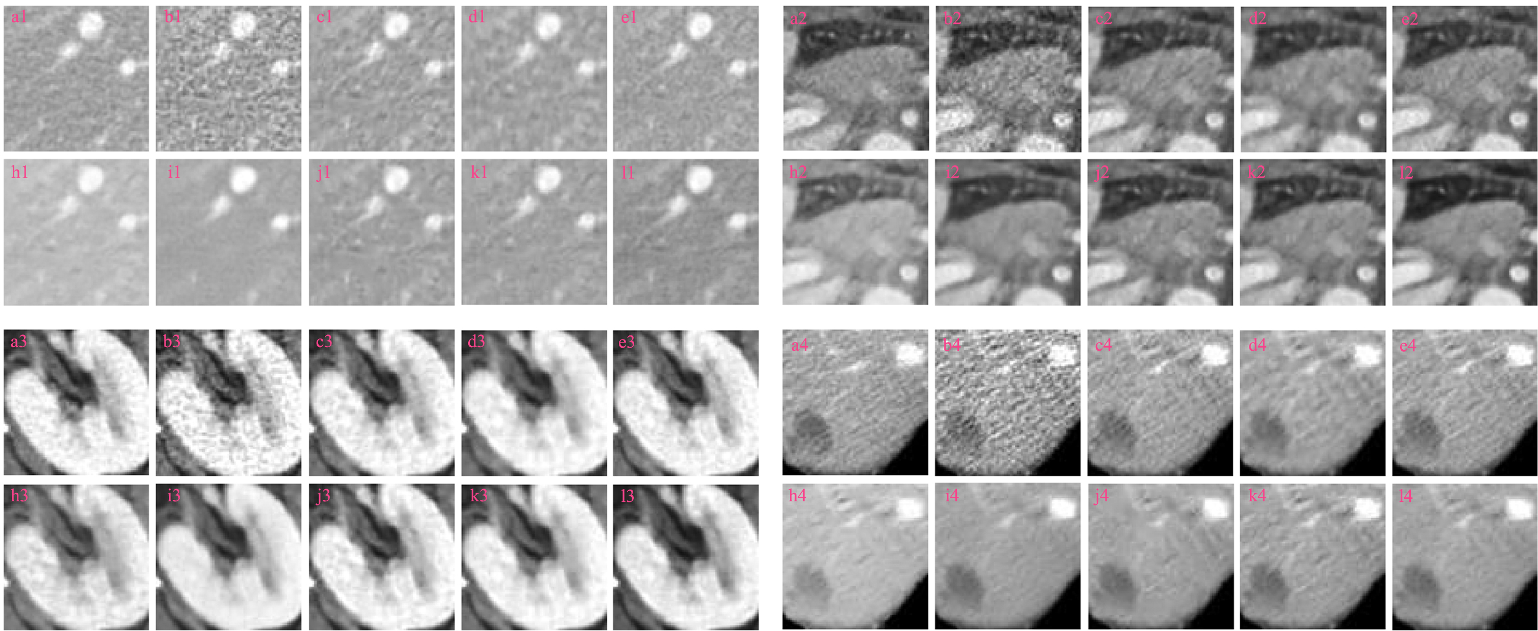
Magnification ROIs.

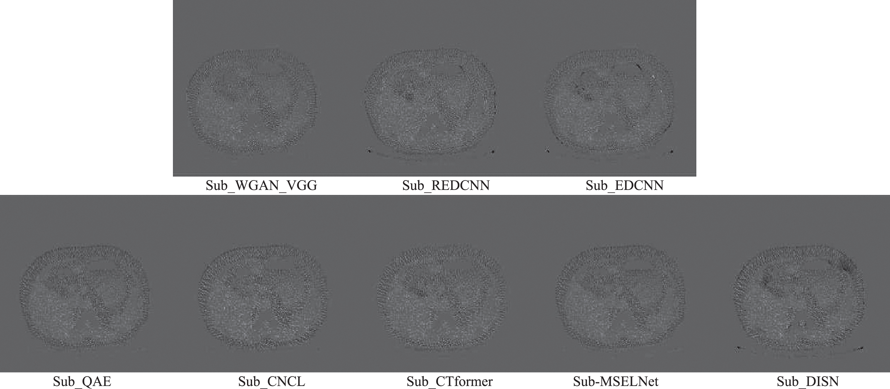
Texture information from CT images is very important for physicians when making a diagnosis. Texture can provide information about the microstructure and the tissue type within the tissue and can help physicians more accurately determine the nature and distribution of lesions. Therefore, it is crucial to suppress artifacts and recover texture and details in LDCT image noise reduction. Figure 10 show the difference images obtained by subtracting different denoised results from LDCT. Evidently, the artifacts (or details) residuals in these difference images can reflect the noise reduction performance of different methods.Among them, the more amount of artifacts (or details) in the difference images, the more amount of artifacts (or details) are suppressed (or damaged) in the noise reduction process. Our study finds that our proposed DISN has a strong noise artifact suppression ability and can suppress the noise to the maximum extent, so its denoising effect is more excellent than other methods.

Fig. 10

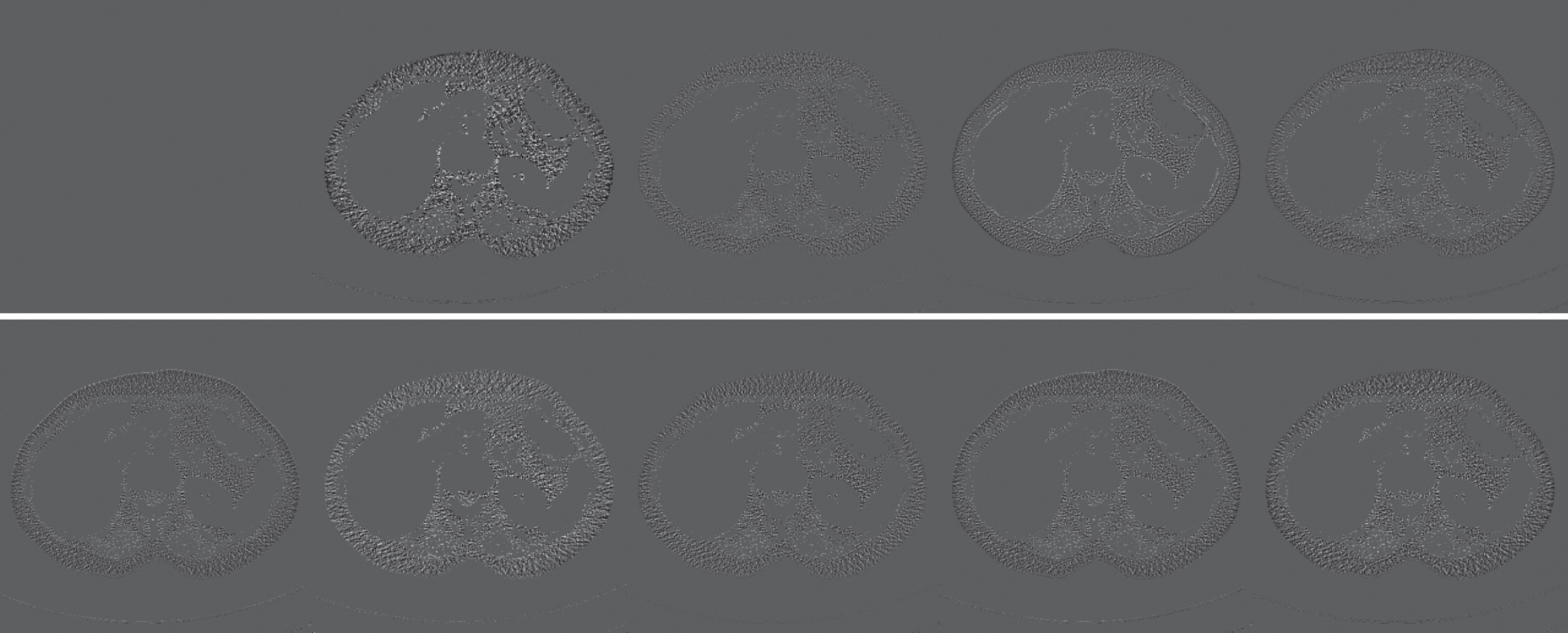
Different methods are used to obtain difference images (Fig. 6).

3.1.3 Quantitative assessment

To quantitatively analyze the effectiveness of different noise reduction methods, Table 1 lists the metrics of these methods for the test data set. The best values are shown in red and the second best values are shown in blue. From the table, DISN shows a more excellent performance in all objective metrics, especially in the two metrics in PSNR and SSIM, where there is a significant improvement. Specifically, WGAN_VGG and CNCL perform poorly in PSNR, while REDCNN and WGAN_VGG score lower in VIFS, which is consistent with excessive image smoothing and low contrast in visual judgment. Although CNCL is at a disadvantage in PSNR, its SSIM and VIFS values still rank second best. both QAE and CT Form CNN-based methods have some advantages. MSELNet performs best in the metrics of FSIM. Although DISN is not the best in the performance index of FSIM, it is not much different from the best MSELNet and performs best in the remaining evaluation indexes, which indicates that the method has the ability of both noise/artifact suppression and feature information retention, and its denoising result is close to the real NDCT image, and its performance is excellent.

Table 1
Comparison with different algorithms on the Aapm Dataset

SSIM↑ PSNR↑ GMSD↓ FSIM↑ VIFS↑

LDCT 0.8585±0.0124 30.2805±0.5197 0.0876±0.0063 0.9452±0.0039 0.4643±0.0157

WGAN_VGG 0.9006±0.0059 32.2831±0.0312 0.0675±0.0020 0.9609±0.0018 0.4970±0.0059

REDCNN 0.9132±0.0074 33.3665±0.3933 0.0584±0.0030 0.9621±0.0023 0.5193±0.0132

EDCNN 0.9081±0.0081 33.2217±0.4164 0.0605±0.0031 0.9614±0.0025 0.5204±0.0138

QAE 0.9161±0.0074 33.6436±0.4001 0.0581±0.0030 0.9625±0.0023 0.5302±0.0137

CNCL 0.9186±0.0064 33.1521±0.5604 0.0636±0.0040 0.9598±0.0022 0.5371±0.0107

CTformer 0.9141±0.0075 33.3942±0.3801 0.0589±0.0030 0.9625±0.0023 0.5259±0.0131

MSELNet 0.9174±0.0053 33.6490±0.3575 0.0585±0.0040 0.9640±0.0100 0.5370±0.0035

DISN 0.9200±0.0070 34.0164±0.3672 0.0578±0.0035 0.9630±0.0021 0.5443±0.0054

	SSIM↑	PSNR↑	GMSD↓	FSIM↑	VIFS↑
LDCT	0.8585±0.0124	30.2805±0.5197	0.0876±0.0063	0.9452±0.0039	0.4643±0.0157
WGAN_VGG	0.9006±0.0059	32.2831±0.0312	0.0675±0.0020	0.9609±0.0018	0.4970±0.0059
REDCNN	0.9132±0.0074	33.3665±0.3933	0.0584±0.0030	0.9621±0.0023	0.5193±0.0132
EDCNN	0.9081±0.0081	33.2217±0.4164	0.0605±0.0031	0.9614±0.0025	0.5204±0.0138
QAE	0.9161±0.0074	33.6436±0.4001	0.0581±0.0030	0.9625±0.0023	0.5302±0.0137
CNCL	0.9186±0.0064	33.1521±0.5604	0.0636±0.0040	0.9598±0.0022	0.5371±0.0107
CTformer	0.9141±0.0075	33.3942±0.3801	0.0589±0.0030	0.9625±0.0023	0.5259±0.0131
MSELNet	0.9174±0.0053	33.6490±0.3575	0.0585±0.0040	0.9640±0.0100	0.5370±0.0035
DISN	0.9200±0.0070	34.0164±0.3672	0.0578±0.0035	0.9630±0.0021	0.5443±0.0054

The distribution characteristics of PSNR and SSIM for the different methods on the test dataset were compared by box-line plots, as shown in Fig. 11. The box line plot sums up the data set with five statistics (maximum, minimum, lower and upper quartiles, and median). Based on the width of the frame and the distribution range of PSNR and SSIM in Fig. 11, we can find that DISN has better robustness compared to other denoising methods. In terms of the grey line (median), the order of different denoising methods is as follows: (PSNR)WGAN < REDCNN < EDCNN < CNCL <CTformer < QAE < MSELNet < DISN,(SSIM)WGAN < EDCNN < REDCNN < CTformer < QAE < CNCL < MSELNet < DISN. DISN has the highest median, which confirms its best performance in terms of average quantization performance.

Fig. 11

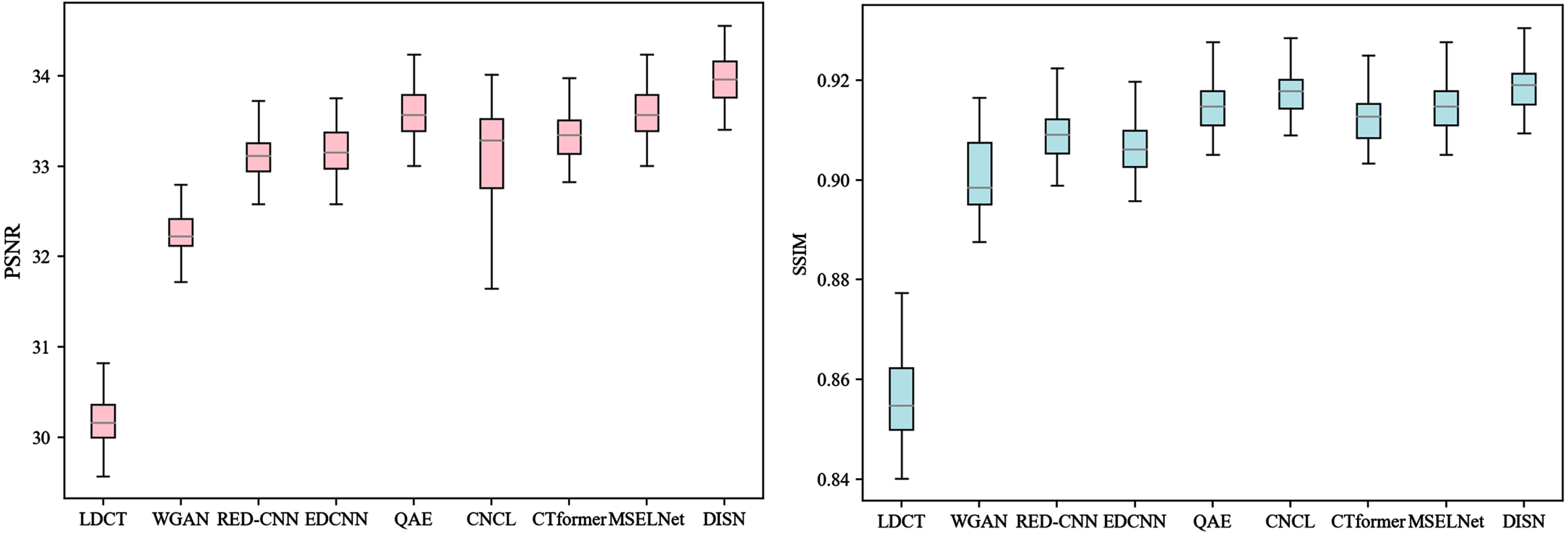
Boxplot of denoised results using different denoising methods on AAPM testing set.

To illustrate that physicians usually focus on the region of interest (ROI) related to medical diagnosis, we use PSNR and SSIM in the figure to quantify the performance of each method within the same ROI, as shown in Fig. 12. Comparing the PSNR of various methods within the same region of interest, it can be found that our proposed DISN is always in the lead and its performance is superior to other methods.

Fig. 12

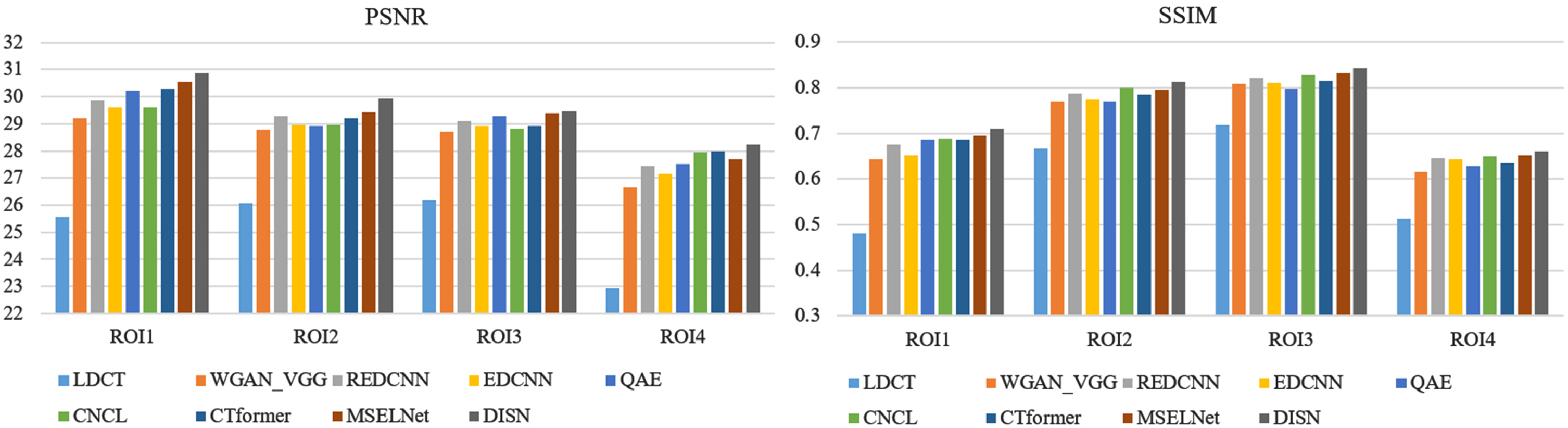
Histogram of ROI of denoised images obtained by different methods.

3.2 Mayo experiments

3.2.1 Experimental details

We obtained a 512×512 piglet CT dataset with different dose ranges of 50%, 25%, 10% and 5% using a Discovery CT750 HD type GE scanner with 300 mAs as the normal dose. We selected 400 pairs of piglet images (tube currents of 150 mAs and 300 mAs, respectively) as training inputs and trained the model. To validate the applicability of the model on different dose datasets, we tested it on four different dose datasets, each containing 40 pairs of images. In evaluating the model performance, we compared the model with five state-of-the-art methods BM3D, REDCNN, EDCNN, QAE, and CT former. We have compared these methods in a comprehensive manner in both visual effectiveness and quantitative evaluation.

3.2.2 Qualitative assessment

In Fig. 13, we display the results of various methods of processing representative piglet sections, which were obtained at different doses of 50%, 25%, 10% and 5%. Since our dataset was trained based on 150 mAs LDCT images, the results obtained by the BM3D method were excessively smooth and the results obtained by the CNN-based method can keep some denoising ability when testing images from datasets with 150 mAs LDCT images and 75 mAs LDCT images. Specifically, the REDCNN, CT form, and QAE methods produce results with blurred details. The EDCNN method preserves edges and details but has inferior denoising performance, while the performance of the DISN network results are very similar to those of the respective NDCT images. The REDCNN method performs well when the test images are from LDCT images at 30 mAs, while our proposed DISN method is closer to the results of NDCT images relative to the other methods. However, when the images are heavily noise-contaminated (15 mAs), all methods fail to achieve satisfactory results, but then the conventional noise reduction method BM3D has some outstanding advantages.

Fig. 13

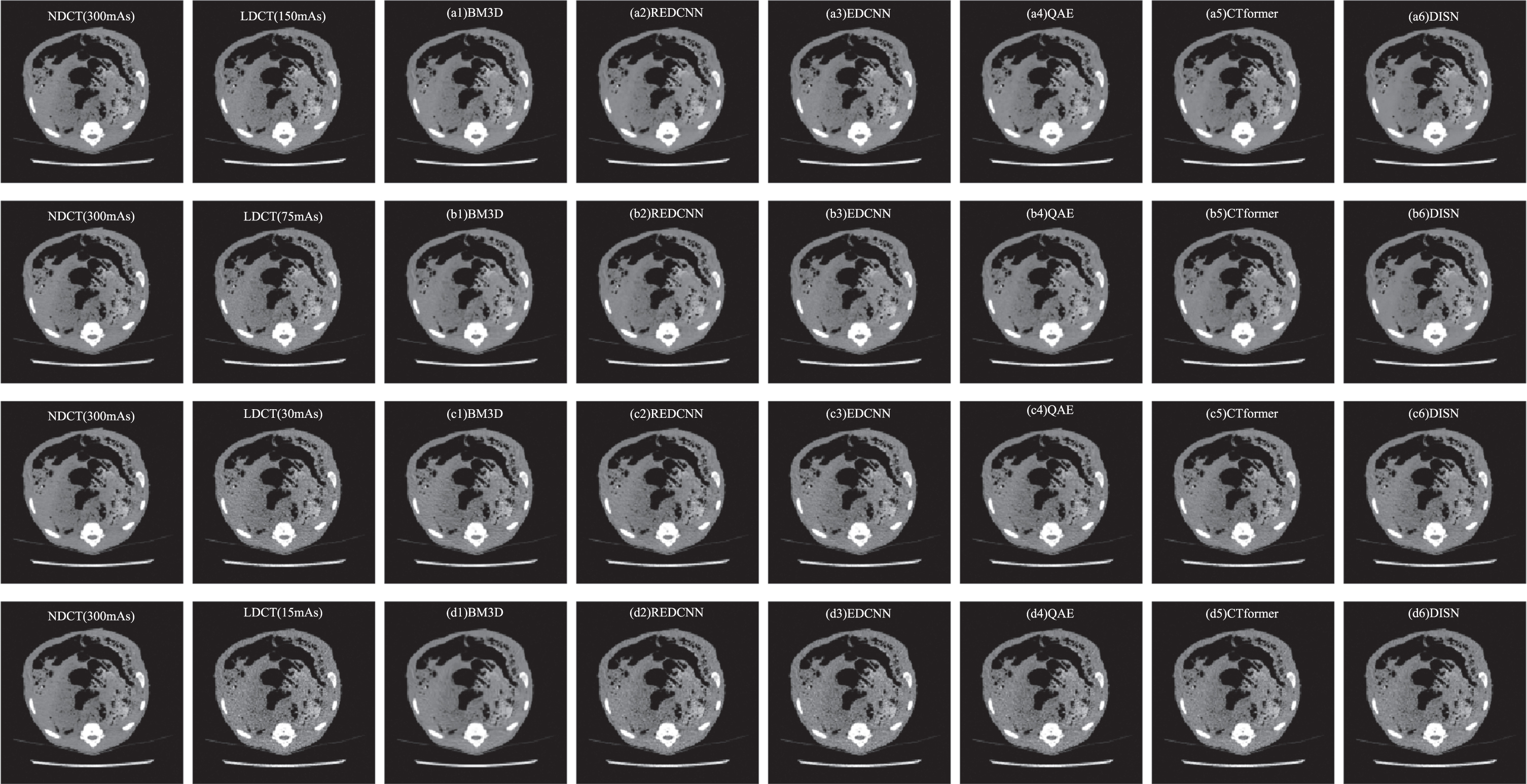
The noise reduction results of the sample in piglet data set are visually displayed.

3.2.3 Quantitative assessment

The average quantitative properties achieved during robustness validation experiments on the whole Piglet dataset are shown in Table 2, where the best and second best values are shown in red and blue. At doses of 50% (150 mA) and 25% (75 mA), the best results for all metrics were achieved with our proposed DISN method. At a dose of 10% (30 mAs), both REDCNN and DISN methods showed good results in all metrics. At 10% dose and 5% dose, conventional denoising method BM3D has the advantage of being unconstrained by the training data set by adjusting the hyperparameters and has better quantitative metrics than the deep learning-based method.

Table 2
Comparison with different algorithms on the Piglet Dataset

DOSE LEVEL METHOD SSIM↑ PSNR↑ GMSD↓ FSIM↑ VIFS↑

50% LDCT 0.9041 31.6362 0.0721 0.9651 0.4657

BM3D 0.9290 32.5492 0.0659 0.9677 0.4794

REDCNN 0.9323 32.8117 0.0685 0.9658 0.4897

EDCNN 0.9237 32.6239 0.0629 0.9692 0.4859

QAE 0.9315 32.6588 0.0672 0.9662 0.4829

CTformer 0.9314 32.8068 0.0680 0.9664 0.4887

DISN 0.9363 33.2140 0.0624 0.9701 0.5104

25% LDCT 0.8683 28.6568 0.1042 0.9429 0.3847

BM3D 0.9079 29.8138 0.0894 0.9509 0.4055

REDCNN 0.9106 30.0259 0.0859 0.9528 0.4168

EDCNN 0.8982 29.8145 0.0868 0.9526 0.4106

QAE 0.9074 29.8093 0.0867 0.9520 0.4074

CTformer 0.9058 29.9176 0.0860 0.9528 0.4106

DISN 0.9154 30.3036 0.0822 0.9583 0.4329

10% LDCT 0.8444 27.8282 0.1296 0.9324 0.3627

BM3D 0.8810 29.6173 0.1035 0.9479 0.3953

REDCNN 0.8929 30.3414 0.0898 0.9547 0.4058

EDCNN 0.8772 29.7752 0.1012 0.9494 0.3974

QAE 0.8842 29.7131 0.0971 0.9505 0.3914

CTformer 0.8782 29.7070 0.0944 0.9514 0.3899

DISN 0.8942 30.0086 0.0882 0.9543 0.4080

5% LDCT 0.8073 25.0477 0.1692 0.9017 0.2922

BM3D 0.8766 28.3753 0.1096 0.9383 0.3388

REDCNN 0.8456 27.1331 0.1361 0.9244 0.3263

EDCNN 0.8323 26.5800 0.1464 0.9181 0.3187

QAE 0.8346 26.4767 0.1452 0.9179 0.3126

CTformer 0.8310 26.5983 0.1387 0.9213 0.3124

DISN 0.8453 27.0593 0.1321 0.9265 0.3201

DOSE LEVEL	METHOD	SSIM↑	PSNR↑	GMSD↓	FSIM↑	VIFS↑
50%	LDCT	0.9041	31.6362	0.0721	0.9651	0.4657
	BM3D	0.9290	32.5492	0.0659	0.9677	0.4794
	REDCNN	0.9323	32.8117	0.0685	0.9658	0.4897
	EDCNN	0.9237	32.6239	0.0629	0.9692	0.4859
	QAE	0.9315	32.6588	0.0672	0.9662	0.4829
	CTformer	0.9314	32.8068	0.0680	0.9664	0.4887
	DISN	0.9363	33.2140	0.0624	0.9701	0.5104
25%	LDCT	0.8683	28.6568	0.1042	0.9429	0.3847
	BM3D	0.9079	29.8138	0.0894	0.9509	0.4055
	REDCNN	0.9106	30.0259	0.0859	0.9528	0.4168
	EDCNN	0.8982	29.8145	0.0868	0.9526	0.4106
	QAE	0.9074	29.8093	0.0867	0.9520	0.4074
	CTformer	0.9058	29.9176	0.0860	0.9528	0.4106
	DISN	0.9154	30.3036	0.0822	0.9583	0.4329
10%	LDCT	0.8444	27.8282	0.1296	0.9324	0.3627
	BM3D	0.8810	29.6173	0.1035	0.9479	0.3953
	REDCNN	0.8929	30.3414	0.0898	0.9547	0.4058
	EDCNN	0.8772	29.7752	0.1012	0.9494	0.3974
	QAE	0.8842	29.7131	0.0971	0.9505	0.3914
	CTformer	0.8782	29.7070	0.0944	0.9514	0.3899
	DISN	0.8942	30.0086	0.0882	0.9543	0.4080
5%	LDCT	0.8073	25.0477	0.1692	0.9017	0.2922
	BM3D	0.8766	28.3753	0.1096	0.9383	0.3388
	REDCNN	0.8456	27.1331	0.1361	0.9244	0.3263
	EDCNN	0.8323	26.5800	0.1464	0.9181	0.3187
	QAE	0.8346	26.4767	0.1452	0.9179	0.3126
	CTformer	0.8310	26.5983	0.1387	0.9213	0.3124
	DISN	0.8453	27.0593	0.1321	0.9265	0.3201

3.3 Real clinic experiments

Due to the more complex noise introduced under natural conditions, we performed robustness validation experiments on real clinical CT images and compared them with relevant comparison experiments. The dataset was approved by the hospital ethics committee. In this section, a representative slice is selected for validation, and two ROI regions from the slice, upper left and upper right, are selected for comparison, as shown in Fig. 14. In the LDCT image, there are severe noise and artifacts that have a significant impact on the observation of texture and lesion. The image after WGAN_VGG processing still has some noise. REDCNN and QAE can suppress noise and artifacts to some extent, but the processed image is blurred. Compared with CT former, EDCNN has more artifacts in the processed images, but the outline of the ROI lesion in the upper right corner is clearer. CNCL and MSELNet can produce better results, but the CNCL processed images still have obvious artifacts and the brightness needs to be improved. Therefore, DISN-processed images are easy to diagnose by physicians and have practical application value.

Fig. 14

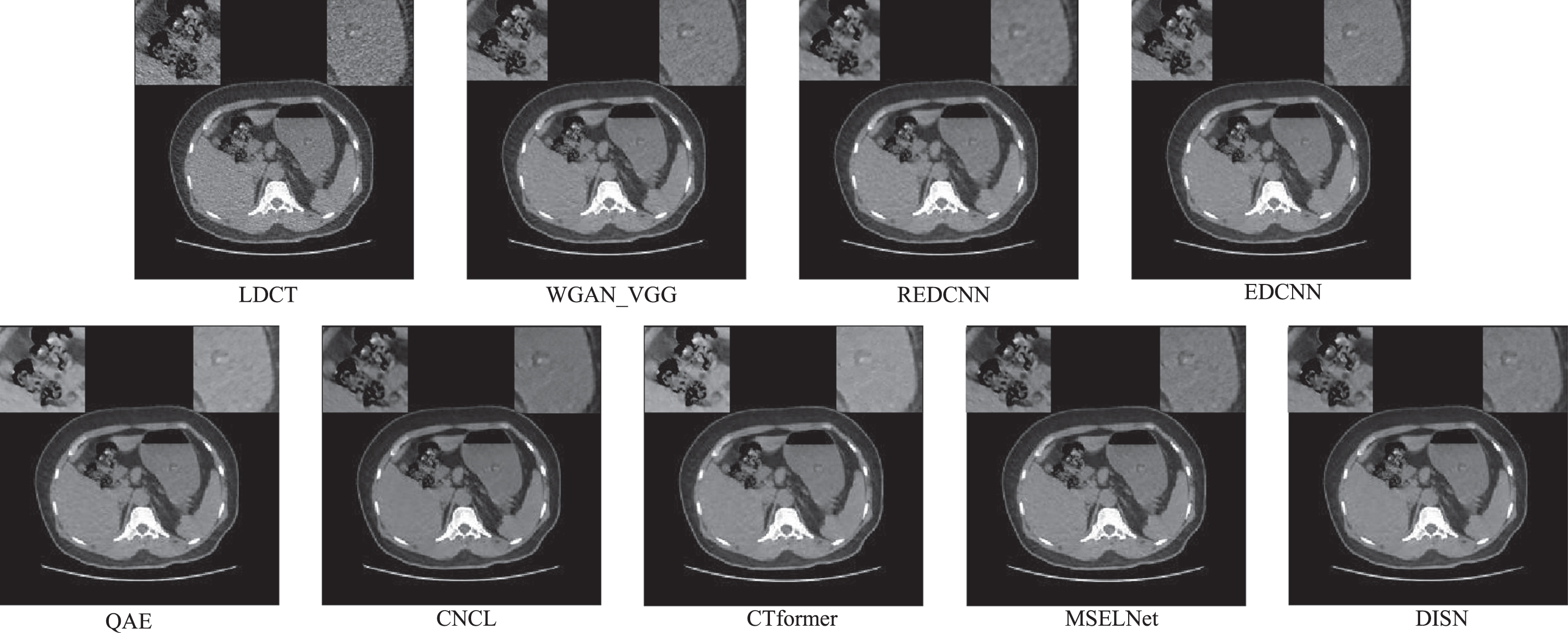
The noise reduction results of the sample in clinic data set are visually displayed.

In LDCT image noise reduction, it becomes particularly important to suppress artifacts and recover texture details. Figure 15 show the difference images obtained by subtracting different denoised results from LDCT. Evidently, the artifacts (or details) residuals in these difference images can reflect the noise reduction performance of different methods. Among them, the more amount of artifacts (or details) in the difference images, the more amount of artifacts (or details) are suppressed (or damaged) in the noise reduction process. Our study finds that our proposed DISN has a strong noise artifact suppression ability and can maximize noise suppression.

Fig. 15

Different methods are used to obtain difference images (Fig. 14).

3.4 Analytical experiments

3.4.1 Number of iterations

We had the number of iterations of DISN models set to 3, 4 and 5 and evaluated their quantitative performance. The experimental results demonstrate that the performance of the DISN model does not improve greatly with increasing the number of iterations, but adds to the number of parameters and training time. Considering the above conditions, the number of iterations of the DISN model is finally set to 3.

3.4.2 Fusion network

By doing 3 iterations, we consider the impact of the fusion network on the whole network. Instead of directly summing the high-frequency information and low-frequency information after obtaining them, our network adds a fusion network to process this information. We selected another representative slice from the Mayo dataset and enlarged the ROI region for better comparison. As can be seen in Fig. 16, if the high-frequency information and low-frequency information are directly summed, the obtained image has some blurring and the details are not obvious.

Fig. 16

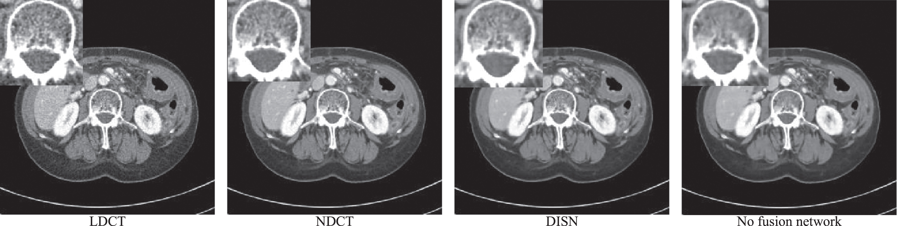
The effect of fusion network on noise reduction of LDCT image.

4 Conclusion

In this study, we proposed a new LDCT image denoising algorithm, interpretable decomposition iterative network (DISN). The algorithm uses a physical model to design a low-dose CT noise reduction network and improves the model’s ability to maintain low-frequency signals and high-frequency details. The purpose is to suppress noise and artifacts caused by radiation dose reduction on CT images. This method solves the blind design or use of deep neural network architecture, combines data-driven and model-driven, solves the unexplained problems inherent in deep learning, and makes full use of data features to make the whole model more reasonable and has better generalization ability. In order to preserve the edge/texture in the iterative process, this paper uses the Hessian matrix to realize the frequency distribution of the image, and designs the corresponding low frequency, high frequency and fusion network. Experiments show that this method can effectively remove the noise and artifacts in CT images, maintain the integrity of CT image structure and pathological information, and improve the diagnostic performance of CT images. Compared with the existing mainstream algorithms, the visualization effect and quantitative indicators of the algorithm are significantly improved, and it has certain generalization ability. However, this method still has some shortcomings. Since the noise in LDCT is distributed over the entire spectrum, if the frequency of the entire noise can be calculated, the accuracy of noise extraction can be improved, thereby further improving the noise reduction ability of LDCT. Although this method has certain interpretability, it still needs to combine the traditional denoising method with the network to design a more accurate and credible method.

Funding

National Nature Science Foundation of China under Grant (61801438), Postgraduate Education Innovation Project of Shanxi Province (2022Y582), the Research Project Supported by Shanxi Scholarship Council of China under Grant 2021-111.

Footnotes

Acknowledgments

We would like to thank the editors and reviewers for their reviews that improved the content of this paper.

Conflict of interest

The authors declare no conflicts of interest.

Data availability

The basic data for the results of this paper can be found in the references.

References

Naidich

D.P.

, Marshall

C.H.

, Gribbin

, Arams

R.S.

, McCauley

D.I.

, Low-dose CT of the lungs: preliminary observations, Radiology 175(3) (1990), pp. 729–31, doi: 10.1148/radiology.175.3.2343122.

Boas

F.E.

, Fleischmann

, CT artifacts: Causes and reduction techniques, Imaging in Medicine 4 (2012), pp. 229–240.

Manduca

, et al. Projection space denoising with bilateral filtering and CT noise modeling for dose reduction in CT, Medical Physics 36(11) (2009), pp. 4911–4919, doi: 10.1118/1.3232004.

Balda

, Hornegger

, Heismann

, Ray Contribution Masks for Structure Adaptive Sinogram Filtering, Ieee Transactions on Medical Imaging 31(6) (2012), pp. 1228–1239, doi: 10.1109/tmi.2012.2187213.

Lee

, et al. A Feasibility Study of Low-Dose Single-Scan Dual-Energy Cone-Beam CT in Many-View Under-Sampling Framework, Ieee Transactions on Medical Imaging 36(12) (2017), pp. 2578–2587, doi: 10.1109/tmi.2017.2765760.

Liu

, Li

, Xiang

, Wang

, Tan

, Low-Dose CBCT Reconstruction Using Hessian Schatten Penalties,–, Ieee Transactions on Medical Imaging 36(12) (2017), pp. 2588–2599, doi: 10.1109/tmi.2017.2766185.

Liu

, et al. 3D Feature Constrained Reconstruction for Low-Dose CT Imaging,–, IEEE Transactions on Circuits and Systems for Video Technology 28(5) (2018), pp. 1232–1247, doi: 10.1109/TCSVT.2016.2643009.

Zhang

, Mou

, Wang

, Yu

, Tensor-Based Dictionary Learning for Spectral CT Reconstruction, Ieee Transactions on Medical Imaging 36(1) (2017), pp. 142–154, doi: 10.1109/tmi.2016.2600249.

Dabov

, Foi

, Katkovnik

, Egiazarian

, Image denoising by sparse 3-D transform-domain collaborative filtering, Ieee Transactions on Image Processing 16(8) (2007), pp. 2080–2095, doi: 10.1109/tip.2007.901238.

10.

Hashemi

, Paul

N.S.

, Beheshti

, Cobbold

R.S.C.

, Adaptively Tuned Iterative Low Dose CT Image Denoising,Art no. 68, Computational and Mathematical Methods in Medicine 2015 (2015), 2015, Art no. 638568, doi: 10.1155/2015/638568.

11.

Huang

, Ma

, Liu

, Feng

, Chen

Projection data restoration guided non-local means for low-dose computed tomography reconstruction, 2011 IEEE International Symposium on Biomedical Imaging: From Nano to Macro, Chicago, IL, USA, (2011), pp. 1167–1170, doi: 10.1109/ISBI.2011.5872609.

12.

Kang

, Slomka

, Nakazato

, Woo

, Berman

D.S.

, Jay Kuo

C.-C.

, Dey

Image denoising of low-radiation dose coronary CT angiography by an adaptive block-matching 3D algorithm, Proc. SPIE 8669, Medical Imaging 2013: Image Processing, 86692G (13 March 2013).

13.

Chen

, et al. Thoracic low-dose CT image processing using an artifact suppressed large-scale nonlocal means, Physics in Medicine and Biology 57(9) 2012, doi: 10.1088/0031-9155/57/9/2667.

14.

YinYong

J.L.

A Non-Local Means Approach for PET Image Denoising. In: Dossel, O., Schlegel, W.C. (eds) World Congress on Medical Physics and Biomedical Engineering, September 7 - 12, 2009, Munich, Germany. IFMBE Proceedings, vol 25/2. Springer, Berlin, Heidelberg (2009). https://doi.org/10.1007/978-3-642-03879-236.

15.

Perona

, Malik

, Scale-space and edge detection using anisotropic diffusion, IEEE Transactions on Pattern Analysis and Machine Intelligence 12(7) (1990), 629–639, doi: 10.1109/34.56205.

16.

Rafsanjani

H.K.

, Sedaaghi

M.H.

, Saryazdi

, An adaptive diffusion coefficient selection for image denoising, Digital Signal Processing 64 (2017), pp. 71–82, doi: 10.1016/j.dsp.2017.02.004.

17.

Yuan

, Improved anisotropic diffusion equation based on new non-local information scheme for image denoising, Iet Computer Vision 9(6) (2015), 864–870, doi: 10.1049/iet-cvi.2014.0415.

18.

Chen

, et al. Improving abdomen tumor low-dose CT images using a fast dictionary learning based processing, Physics in Medicine and Biology 58(16) (2013), pp. 5803–5820, doi: 10.1088/0031-9155/58/16/5803.

19.

, Zhang

, Multiscale Wiener filtering method for low-dose CT images, 3rd International Conference on Biomedical Engineering and Informatics, Yantai, China (2010), pp. 428–431, doi: 10.1109/BMEI.2010.5639560.

20.

Chen

, et al. Low-Dose CT With a Residual Encoder-Decoder Convolutional Neural Network, Ieee Transactions on Medical Imaging 36(12) (2017), pp. 2524–2535, doi: 10.1109/tmi.2017.2715284.

21.

Fan

, et al. Quadratic Auto encoder (Q-AE) for Low-Dose CT Denoising, Ieee Transactions on Medical Imaging 39(6) (2020), pp. 2035–2050, doi: 10.1109/tmi.2019.2963248.

22.

Kang

, Min

, Ye

J.C.

, A deep convolutional neural network using directional wavelets for low-dose X-ray CT reconstruction, Medical Physics 44(10) (2017), pp. e360–e375, doi: 10.1002/mp.12344.

23.

Liang

, Jin

, Li

, Wang

, EDCNN: Edge enhancement-based Densely Connected Network with Compound Loss for Low-Dose CT Denoising, 2020 15th IEEE International Conference on Signal Processing (ICSP), Beijing, China (2020), pp. 193–198, doi: 10.1109/ICSP48669.2020.9320928.

24.

Jiang

, Wang

, He

, Du

, Learning a Frequency Separation Network with Hybrid Convolution and Adaptive Aggregation for Low-dose CT Denoising, 2021 IEEE International Conference on Bioinformatics and Biomedicine (BIBM), Houston, TX, USA (2021), pp. 919–925, doi: 10.1109/BIBM52615.2021.9669891.

25.

Gholizadeh-Ansari

, Alirezaie

, Babyn

, Deep Learning for Low-Dose CT Denoising Using Perceptual Loss and Edge Detection Layer, Journal of Digital Imaging 33(2) (2020), pp. 504–515, doi: 10.1007/s10278-019-00274-4.

26.

, et al. Multi-Scale Feature Fusion Network for Low-Dose CT Denoising, Journal of Digital Imaging Early Access 2023, doi: 10.1007/s10278-023-00805-0.

27.

Wolterink

J.M.

, Leiner

, Viergever

M.A.

, Igum

, Generative adversarial networks for noise reduction in low-dose CT, IEEE Transactions on Medical Imaging 36(12) (2017), 2536–2545, doi: 10.1109/TMI.2017.2708987.

28.

Yang

, et al. Low-Dose CT Image Denoising Using a Generative Adversarial Network With Wasserstein Distance and Perceptual Loss, Ieee Transactions on Medical Imaging 37(6) (2018), pp. 1348–1357, doi: 10.1109/tmi.2018.2827462.

29.

Geng

, et al. Content-Noise Complementary Learning for Medical Image Denoising, Ieee Transactions on Medical Imaging 41(2) (2022), pp. 407–419, doi: 10.1109/tmi.2021.3113365.

30.

Han

, Shangguan

, Zhang

, Cui

, Ren

, A Dual-Encoder-Single-Decoder Based Low-Dose CT Denoising Network, Ieee Journal of Biomedical and Health Informatics 26(7) (2022), pp. 3251–3260, doi: 10.1109/jbhi.2022.3155788.

31.

Marcos

, Alirezaie

, Babyn

Low Dose CT Image Denoising Using Boosting Attention Fusion GAN with Perceptual Loss, 2021 43rd Annual International Conference of the IEEE Engineering in Medicine & Biology Society (EMBC), Mexico, (2021), pp. 3407–3410, doi: 10.1109/EMBC46164.2021.9630790.

32.

Lyu

, Fu

, Peng

, Zhou

S.K.

U-DuDoNet: Unpaired Dual-Domain Network for CT Metal Artifact Reduction. In: de Bruijne, M., et al. Medical Image Computing and Computer Assisted Intervention –MICCAI 2021. MICCAI 2021. Lecture Notes in Computer Science(), vol 12906. Springer, Cham. (2021). https://doi.org/10.1007/978-3-030-87231-129.

33.

Yin

, et al. Domain Progressive 3D Residual Convolution Network to Improve Low-Dose CT Imaging, Ieee Transactions on Medical Imaging 38(12) (2019), pp. 2903–2913, doi: 10.1109/tmi.2019.2917258.

34.

Wang

, Fan

, Wu

, Liu

, Wang

, Yu

CTformer: Convolution-free Token2Token Dilated Vision Transformer for Low-dose CT Denoising, arXiv preprint arXiv:2202.13517, 2022.

35.

McCollough

, Overview of the Low Dose CT Grand Challenge, Medical Physics 43(6) (2016), pp. 3759–3760, doi: 10.1118/1.4957556.

36.

Piglet Dataset. [Online]. Available: http://homepage.usask.ca/?xiy525/publication/sagan/.

37.

Wang

, Bovik

A.C.

, Sheikh

H.R.

, Simoncelli

E.P.

, Image quality assessment: from error visibility to structural similarity, IEEE transactions on image processing: a publication of the IEEE Signal Processing Society 13(4) (2004), pp. 600–612, doi: 10.1109/tip.2003.819861.

38.

Xue

, Zhang

, Mou

, Bovik

A.C.

, Gradient Magnitude Similarity Deviation: A Highly Efficient Perceptual Image Quality Index, Ieee Transactions on Image Processing 23(2) (2014), pp. 684–695, doi: 10.1109/tip.2013.2293423.

39.

Zhang

, Zhang

, Mou

, Zhang

, FSIM: A Feature Similarity Index for Image Quality Assessment, Ieee Transactions on Image Processing 20(8) (2011), pp. 2378–2386, doi: 10.1109/tip.2011.2109730.

40.

Sheikh

H.R.

, Bovik

A.C.

, Image information and visual quality, IEEE transactions on image processing: a publication of the IEEE Signal Processing Society 15(2) (2006), pp. 430–44, 2006-Feb 2006, doi: 10.1109/tip.2005.859378.