Expected Anomalies in the Fossil Record

Abstract

The problem of intermediates in the fossil record has been frequently discussed ever since Darwin. The extent of ‘gaps’ (missing transitional stages) has been used to argue against gradual evolution from a common ancestor. Traditionally, gaps have often been explained by the improbability of fossilization and the discontinuous selection of found fossils. Here we take an analytical approach and demonstrate why, under certain sampling conditions, we may not expect intermediates to be found. Using a simple null model, we show mathematically that the question of whether a taxon sampled from some time in the past is likely to be morphologically intermediate to other samples (dated earlier and later) depends on the shape and dimensions of the underlying phylogenetic tree that connects the taxa, and the times from which the fossils are sampled.

Keywords

fossil record null models phylogenetic trees

Introduction

Since Darwin's book On the Origin of Species by Means of Natural Selection, or the Preservation of Favoured Races in the Struggle for Life [2], there has been much debate about the evidence for continuous evolution from a universal common ancestor. Initially, Darwin only assumed the relatedness of the majority of species, not of all of them; later, however, he came to the view that because of the similarities of all existing species, there could only be one ‘root’ and one ‘tree of life’ (cf. [11]). All species are descended from this common ancestor and indications for their gradual evolution have been sought in the fossil record ever since. Usually, the improbability of fossilization or of finding existing fossils was put forward as the standard answer to the question of why there are so many ‘gaps’ in the fossil record. Such gaps have become popularly referred to as ‘missing links’, i.e. missing intermediates between taxa existing either today or as fossils.

Of course, the existence of gaps is in some sense inevitable: every new link gives rise to two new gaps, since evolution is generally a continuous process whereas fossil discovery will always remain discontinuous. Moreover, a patchy fossil record is not necessarily evidence against evolution from a common ancestor through a continuous series of intermediates—indeed, in a recent approach, Elliott Sober (cf. [11]) applied simple probabilistic arguments to conclude that the existence of some intermediates provides a stronger support for evolution than the non-existence of any (or some) intermediates could ever provide for a hypothesis of separate ancestry. Moreover, some lineages appear to be densely sampled, whereas of others only few fossiliferous horizons are known (cf. [10]). This problem has been well investigated and statistical models have been developed to master it (see e.g. [6, 7]), [12]).

In this paper, we suggest a further argument that may help explain missing links in the fossil record. Suppose that three fossils can be dated back to three different times. Can we really expect that a fossil from the intermediate time will appear (morphologically) to be an ‘intermediate’ of the other two fossils? We will explore this question via a simple stochastic model.

In order to develop this model, we first state some assumptions we will make throughout this paper: firstly, we will consider that we are sampling fossil taxa of closely related organisms and which differ in a number of morphological characteristics. We assume this group of taxa has evolved in a ‘tree-like’ fashion from some common ancestor; that is, there is an underlying phylogenetic tree, and the taxa are sampled from points on the branches of this tree.

It is also necessary to say how morphological divergence might be related to time, as this is important for deciding whether a taxon is an intermediate or not. In this paper, we make the simplifying assumption that, within the limited group of taxa under consideration (and over the limited time period being considered), the expected degree of morphological divergence between two taxa is proportional to the total amount of evolutionary history separating those two taxa. This evolutionary history is simply the time obtained by adding together the two time periods from the most recent common ancestor of the two taxa until the times from which each was sampled (in the case where one taxon is ancestral to the other, this is simply the time between the two samples). This assumption on morphological diversity would be valid (in expectation) if we view morphological distance as being proportional to the number of discrete characters that two species differ on, provided that two conditions hold: (i) each character has a constant rate of character state change (substitution) over the time frame T that the fossils are sampled from, and (ii) T is short enough that the probability of a reverse or convergent change at any given character is low. We require these conditions to hold in the proofs of the following results. We will discuss other possible relations of morphological diversification and distance towards the end of this paper.

The simplest scenario is the case where the three samples all lie on the same lineage, so that the evolutionary tree can be regarded as a path (cf. Fig. 1). In this case, the path distance (and hence expected morphological distance) between the outer two fossils is always larger than the distance that either of them has from the fossil sampled from an intermediate time. But for samples that straddle bifurcations in a tree, it is quite easy to imagine how this intermediacy could fail; for example, if the two outer taxa lie on one branch of the tree and the fossil from the intermediate time lies on another branch far away (cf. Fig. 2). But this example might be unlikely to occur, and indeed we will see that if sampling is uniform across the tree at any given time, in expectation the morphological distances remain intermediate even for this case (cf. Fig. 2). Yet for more complex trees, this expected outcome can fail, and perhaps most surprisingly, the distance between the earliest and latest sample can, in expectation, be the smallest of the three distances in certain extreme cases.

Figure 1.

When the tree consists of only one lineage from which samples are taken at times T₁, T₂ and T₃, then clearly the distance d_1,3 is always larger than d_1,2 and d_2,3. Consequently, E₁ ₃ > max{E_1,2, E_2,3}.

Figure 2.

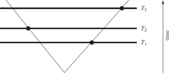
For samples taken from different lineages of a tree, the distance d_1,3 of one particular sample from time T₁ to the one of T₃ can be smaller than the distance of either of them to the sample taken at time T₂. Yet in expectation we always have E₁₃ > max{E_1,2, E_2,3} for two-branch trees. For more complex trees this can fail as we show in Example 2.7.

Thus, in order to make general statements, we will consider the expected degree of relatedness of fossils sampled randomly from given times. Our results will depend solely on the tree shape (including branch lengths) of the underlying tree and the chosen times.

Results

We begin with some notation. Throughout this paper, we assume a rooted binary phylogenetic tree to be given with an associated time scale 0 < T₁ < T₂ < T₃. The number of T_i-lineages (of lineages extant at time T_i) is denoted by n_i. For instance, in Figure 3, the number n₁ of T₁-lineages is 3, whereas the numbers n₂ and n₃ of T₂- and T₃-lineages are both 5. If not stated otherwise, extinction may occur in the tree. Every bifurcation in the tree is denoted by b₁, where b₀ is the root. Note that in a tree without extinction, the total number of bifurcations up to time T₃ (including the root) is n₃ − 1. For every b_i let t_i denote the time of the occurrence of bifurcation b_t. We may assume that the root is at time t₀ = 0.

Figure 3.

A rooted binary phylogenetic tree with three times T₁, T₂, T₃ at which taxa have been sampled. The dotted branches refer to taxa that do not contribute to the expected distances from one of these times to another and thus are not taken into account. On the other hand, bifurcation b₂ at time t₂ shows that extinction may have an impact on the expected values. Such branches have to be considered.

Now, for every b_i, we make the following definitions:

P_{i}^{j, k} : n_{j, i}^{l} . n_{k, i}^{r} + n_{j, i}^{r} . n_{k, i}^{l}

for all

j, k \in {1, 2, 3}, j \neq k

where

n_{j, i}^{r}

denotes the number of descendants the subtree with root b_i has at time T_j to the left of its root b_i, and

n_{j, i}^{l}

is defined analogously for the descendants on the right hand side of b_i.

It can be seen that bifurcations for which at least one branch of offspring dies out in the same interval where the bifurcation lies always have $P_{i}^{j, k}$ value 0. Consequently, if either t₀ < t_i < T_i or T_i < t_i < T₂ or T₂ < t_i < T₃ and one of b_i's branches becomes extinct in the same interval, respectively, then $P_{i}^{j, k}$ is 0 for all j, k. Note that the number $P_{i}^{j, k}$ denotes the number of different paths in the tree from time T_j to time T_k in the subtree with root b_i and in which no edge is taken twice.

Example 2.1

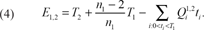
Consider the tree given in Figure 3. Here, the values $P_{i}^{j, k}$ for bifurcation b₁ corresponding to time t₁ are $P_{i}^{1, 2} = n_{1, 1}^{l} \cdot n_{2, 1}^{r} + n_{1, 1}^{r} \cdot n_{2, 1}^{l} = 1 \cdot 2 + 1 \cdot 1 = 3$ , $P_{1}^{1, 3} = 1 \cdot 3 + 1 \cdot 1 = 4$ and $P_{1}^{2, 3} = 1 \cdot 3 + 2 \cdot 1 = 5$ .

In the sampling, select uniformly at random one of the T_i-lineages as well as one of the T_j-lineages to get the expected length E_{i, j} of the path connecting a lineage at time T_i with one at time T_j in the underlying phylogenetic tree. Then, the expectation that a fossil from the intermediate time T₂ also will be an intermediate taxon of two taxa taken from T₁ and T₃, respectively, refers to the assumption that E_1,3 > max {E_1,2, E_2,3}. We will show in the following lemma that this last inequality can fail and describe the precise condition for this to occur. Moreover, we later show that E_1,3 can be strictly smaller (!) than both E_1,2 and E_2,3—that is the temporally most distant samples can, on average, be more similar than the temporally intermediate sample is to either of the two.

Note that if $P_{i}^{j, k}$ is 0, the corresponding branch does not contribute to the expected distance from one time to another. We can therefore assume without loss of generality that all bifurcations b_i have at least one descendant on their left-hand side and at least one on their right-hand side, each in at least one of the times T₁, T₂, T₃. In Figure 3, branches that therefore need not be considered are represented with dotted lines.

In order to simplify the statement of our results, for all bifurcations b_i set

Q_{i}^{j, k} : = \frac{2. P_{i}^{j, k}}{n_{j} n_{k}}

for all

j, k \in {1, 2, 3}, j \neq k

Lemma 2.2

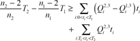
Given a rooted binary phylogenetic tree with times 0 < T₁ < T₂ < T₃ and the root at time t₀ = 0. Then, E_1,3 ≤ E_1,2 if and only if

T_{3} - T_{2} \leq \sum_{i : 0 < t_{i} < T_{1}} (Q_{i}^{1, 3} - Q_{i}^{1, 2}) t_{i}

Proof.

E_{1, 3} = \frac{1}{n_{1} n_{3}} [\underset{\begin{array}{l} every T_{3} - lineage \\ has an ancestor in T_{1} \end{array}}{\underset{︸}{n_{3} (T_{3} - T_{1})}} + \sum_{i : 0 < t_{i} < T_{1}} [P_{i}^{1, 3} (T_{3} - T_{1} + 2 (T_{1} - t_{i}))] + \underset{ways along the root}{\underset{︸}{P_{0}^{1, 3} (T_{3} + T_{1})}}]

(1)

In the above bracket, the three summands refer to different paths from time T₁ to time T₃. The first summand belongs to those paths that go directly from T₁ to T₃ and thus have length T₃–T₁. There are n₃ such ways as every T₃-lineage has an ancestor in T₁. The second summand sums up all paths going along one of the bifurcations b_i for i ≠ 0. For every i, there are by definition exactly $P_{i}^{1, 3}$ such paths. Similarly, the third summand refers to all paths along the root b₀, whose length is determined by taking the distance from T₁ to the root plus the distance from there to T₃.

As there are altogether n₁n₃ different paths from T₁ to T₃ in the tree, we have:

n_{3} + \sum_{i : 0 < t_{i} < T_{1}} P_{i}^{1, 3} + P_{0}^{1, 3} = n_{1} n_{3} .

(2)

Then, by (1) and (2), we get

E_{1, 3} = \frac{1}{n_{1}} . \frac{1}{n_{3}} . (n_{1} n_{3} T_{3} + (n_{1} n_{3} - 2 n_{3}) T_{1} - 2. \sum_{i : 0 < t_{i} T_{1}} P_{i}^{1, 3} t_{i}),

and thus

E_{1, 3} = T_{3} + \frac{n_{1} - 2}{n_{1}} T_{1} - \sum_{i : 0 < t_{i} < T_{1}} Q_{i}^{1, 3} t_{i} .

(3)

Analogously,

E_{1, 2} = T_{2} + \frac{n_{1} - 2}{n_{1}} T_{1} - \sum_{i : 0 < t_{i} < T_{1}} Q_{i}^{1, 2} t_{i} \cdot

(4)

Thus, with (3) and (4), we can conclude:

\begin{array}{l} E_{1, 3} \leq E_{1, 2} & \Leftrightarrow T_{3} - & \sum_{i : 0 < t_{i} < T_{1}} Q_{i}^{1, 3} t_{i} & \leq T_{2} - \sum_{i : 0 < t_{i} < T_{1}} Q_{i}^{1, 2} t_{i} \\ \Leftrightarrow & T_{3} - T_{2} & \leq \sum_{i : 0 < t_{i} < T_{1}} (Q_{i}^{1, 3} - Q_{i}^{1, 2}) t_{i} . \end{array}

Corollary 2.3

For a given tree there exist times 0 > T₁ < T₂ < T₃ such that E_1,3 ≤ E_1,2 if and only if $\sum_{i : 0 < t_{i} < T_{1}} (Q_{i}^{1, 3} - Q_{i}^{1, 2}) t_{i} > 0$ .

Proof. If, $\sum_{i : 0 < t_{i} < T_{1}} (Q_{i}^{1, 3} - Q_{i}^{1, 2}) t_{i} \leq 0$ , then by Lemma 2.2 we need T₂ ≥ T₃ in order to get E_1,3 ≤ E_1,2. Hence, there are no values 0 < T₁ < T₂ < T₃ such that T₃ – T₂ fulfills the required condition, and so E_1,3 > E_1,2 for all choices of T_i. Conversely, suppose $\sum_{i : 0 < t_{i} < T_{1}} (Q_{i}^{1, 3} - Q_{i}^{1, 2}) t_{i} > 0$ . Then, select T₁, T₂ with 0 < T₁ < T₂ and set

T_{3} : = \frac{1}{2} \cdot \sum_{i : 0 < t_{i} < T_{1}} (Q_{i}^{1, 3} - Q_{i}^{1, 2}) t_{i} + T_{2}

Then, T₃ > T₂ and

T_{3} - T_{2} = \frac{1}{2} \cdot \sum_{i : 0 < t_{i} T_{1}} (Q_{i}^{1, 3} - Q_{i}^{1, 2}) t_{i} \leq \sum_{i : 0 < t_{i} < T_{1}} (Q_{i}^{1, 3} - Q_{i}^{1, 2}) t_{i} \cdot

By Lemma 2.2, this choice of 0 < T₁ < T₂ < T₃ leads to E_1,3 ≤ E_1,2.

Corollary 2.4

If either (i) n₁ = 2 or (ii) no extinction occurs in the tree and n₂ = n₃, then E_1,3 > E_1,2.

Proof, (i) Note that if n₁ = 2, obviously only one bifurcation, say b_î (for some î such that 0 ≤ t_î < T₁), contributes to the number n₁ of lineages at time T₁, all the branches added by additional bifurcations become extinct before T₁. Thus: $P_{\hat{i}}^{1, 3}$ , $P_{\hat{i}}^{1, 2} \neq 0$ and $P_{\hat{i}}^{1, 3}$ , $P_{\hat{i}}^{1, 2} = 0$ for all i ≠ î. Analogously to the proof of Lemma 2.2 we have for n₁ = 2: n₁n₃ = 2n₃ = n₃ + $P_{\hat{i}}^{1, 3}$ and n₁n₂ = 2n₂ = n₂ + $P_{\hat{i}}^{1, 2}$ . Thus, n₂ = $P_{\hat{i}}^{1, 2}$ and n₃ = $P_{\hat{i}}^{1, 3}$ .

Therefore, $Q_{\hat{i}}^{1, 2} = Q_{\hat{i}}^{1, 3} = 2 / n_{1}$ and $Q_{\hat{i}}^{1, 2} = Q_{\hat{i}}^{1, 3} = 0$ for all î ≠ î Thus, $\sum_{i : 0 < t_{i} < T_{1}} (Q_{i}^{1, 3} - Q_{i}^{1, 2}) t_{i} > 0$ and it follows with Corollary 2.3 that E_1,3 > E_1,2. (ii) In this case, obviously $(Q_{i}^{1, 2} - Q_{i}^{1, 3})$ for all i : 0 < t_i < T₁ and therefore $\sum_{i : 0 < t_{i} < T_{1}} (Q_{i}^{1, 3} - Q_{i}^{1, 2}) t_{i} = 0$ .

Thus, by Corollary 2.3, E_1,3 > E_1,2.

Lemma 2.2 essentially states that the expected degree of relatedness from taxa of time T₁ to taxa of time T₃ can be larger than the one to taxa of time T₂, but it requires the distance from T₂ to T₃ to be “small enough”. Whether such a solution is feasible can be checked via Corollary 2.3. Lemma 2.2 shows already how the role of intermediates depends on the times the fossils are taken from. Corollary 2.4(i) on the other hand shows how the tree itself has an impact on the expected values: if the tree shape (including branch lengths) is such that at time T₁ only two taxa exist, then the just mentioned scenario cannot happen as the condition of Corollary 2.3 is not fulfilled.

However, we can prove an even stronger result, namely that not only E_1,3 < E_1,2 is possible, but E_1,3 < min {E_1,2, E_2,3) can be obtained for a suitable choice of times T₁, T₂, T₃. For this, we need the following lemma.

Lemma 2.5

Given a rooted binary phylogenetic tree with times 0 < T₁ < T₂ < T₃ and the root at time t₀ = 0. Then E_1,3 ≤ E_2,3 if and only if

\frac{n_{2} - 2}{n_{2}} T_{2} - \frac{n_{1} - 2}{n_{1}} T_{1} \geq \sum_{i : 0 < t_{i} < T_{1}} (Q_{i}^{2, 3} - Q_{i}^{1, 3}) t_{i} + \sum_{i : T_{1} < t_{i} < T_{2}} Q_{i}^{2, 3} t_{i}

Proof. As in the proof of Lemma 2.2, we have (cf (3))

E_{1, 3} = T_{3} + \frac{n_{1} - 2}{n_{1}} T_{1} - \sum_{i : 0 < t_{i} < T_{1}} Q_{i}^{1, 3} t_{i} .

(5)

Analogously,

E_{2, 3} = T_{3} + \frac{n_{2} - 2}{n_{2}} T_{2} - \sum_{i : 0 < t_{i} < T_{1}} Q_{i}^{2, 3} t_{i} .

(6)

Thus, E_1,3 ≤ E_2,3 if and only if

\frac{n_{1} - 2}{n_{1}} T_{1} - \sum_{i : 0 < t_{i} < T_{1}} Q_{i}^{1, 3} \leq \frac{n_{2} - 2}{n_{2}} T_{2} - \sum_{i : 0 < t_{i} < T_{1}} Q_{i}^{2, 3} t_{i},

which holds precisely if

\frac{n_{2} - 2}{n_{2}} T_{2} - \frac{n_{1} - 2}{n_{1}} T_{1} \geq \sum_{i : 0 < t_{i} < T_{1}} (Q_{i}^{2, 3} - Q_{i}^{1, 3}) t_{i} + \sum_{i : T_{1} < t_{i} < T_{2}} Q_{i}^{2, 3} t_{i} .

With the help of the two lemmas we can now state the following theorem.

Theorem 2.6

Given a rooted binary phylogenetic tree with times 0 < T₁ < T₂ < T₃ and the root at time 0. Then, E_1,3 ≤ min {E_1,2, E_2,3} if and only if the following two conditions hold.

(i)

T_{3} - T_{2} \leq \sum_{i : 0 < t_{i} < T_{1}} (Q_{i}^{1, 3} - Q_{i}^{1, 2}) t_{i},

(ii)

\frac{n_{2} - 2}{n_{2}} T_{2} - \frac{n_{1} - 2}{n_{1}} T_{1} \geq \sum_{i : 0 < t_{i} < T_{1}} (Q_{i}^{2, 3} - Q_{i}^{1, 3}) t_{i} + \sum_{i : T_{1} < t_{i} < T_{2}} Q_{i}^{2, 3} t_{i} .

Proof. The Theorem follows directly from Lemmas 2.2 and 2.5.

The following example demonstrates the influence of times 0 < T₁ < T₂ < T₃ according to the above theorem.

Example 2.7

Consider again Figure 3.

(1) Assume t₁ = 15, T₁ = 100, t₂ = 107, t₃ = 109, T₂ = 110, T₃ = 130. Then, E_1,2 = 137.33, E_2,3 = 155.28 and E_1,3 = 155.33. Hence, for this choice of times, we have E_1,3> max{E_1,2, E_2,3}.

(2) Consider the same times as in the previous case, but choose T₂ = 129 instead of T₂ = 110. This means to move T₂ further away from T₁ and closer to T₃. This change is enough to give completely different expected values: E_1,2 = 156.33, E_2,3 = 166.68 and E_1,3 = 155.33. Hence, for this choice of times, we have E_1,3 < min {E_1,2, E_2,3}.

Discussion

The analysis of the fossil record provides an insight into the history of species and thus into evolutionary processes. Stochastic models can provide a useful way to infer patterns of diversification, and they form a useful link between molecular phylogenetics and paleontology [8]. Such models would greatly benefit from incorporation of potential fossil ancestors and other extinct data points to infer patterns of evolution. In this paper we have applied a simple model-based phylogenetic approach to study the expected degree of similarity between fossil taxa sampled at intermediate times.

‘Gaps’ in the fossil record are problematic [10] as they can be interpreted as ‘missing links’. Therefore, numerous studies concerning the adequacy of the fossil record have been conducted (see, for example, [3, 9, 13]), and it is frequently found that even the available fossil record is still incompletely understood. This is particularly true for ancestor-descendant relationships (see, for instance, [4, 5]). For example Foote [5] reported the probability that a preserved and recorded species has at least one descendant species that is also preserved and recorded is on the order of 1%–10%. This number is much higher than the number of identified ancestor-descendant pairs. Thus, it remains an important challenge to recognize such pairs [1]. This is also essential with regard to ancestor-intermediate-descendant triplets, as it is possible that there are in fact fewer ‘gaps’ than currently assumed, i.e. that intermediates are present but not yet recognized. Such issues have an important bearing on any conclusions our results might imply concerning the testing of hypotheses of continuous morphological evolution, or concerning the shape of the underlying evolutionary tree based on the non-existence of certain intermediates.

Another challenge is to investigate different phylogenetic models for describing the expected degree of morphological separation between different fossil taxa sampled at different times. Our findings strongly depend on the assumption that morphological diversification is proportional to the distance in the underlying phylogenetic tree. This is justified if morphological difference is proportional to the number of differing discrete characters, that each of these characters changes at a constant rate over the time period of sampling, and that homoplasy is rare. This last assumption requires the rate of character change to be sufficiently small in relation to the time period of the sampling—the appearance of reverse or convergent character states will lead to a more concave (rather than linear) relationship between morphological divergence and path distance. A similar concave relationship might be expected for continuous morphological evolution as described by neutral Brownian-motion.

Thus, the impact of different assumptions on the role of intermediates could be further investigated. But even if we assume that diversification is proportional to time, there may be other ways to measure ‘distance’ that could be usefully explored—for instance, one could define the distance between two taxa to be the maximum (rather than the sum) of the two divergence times of the taxa back to their most recent common ancestor. This definition of distance allows the degree of relatedness to be higher for taxa on the same clade than for other taxa. In this case, there exist analogous results to Lemmas 2.2 and 2.5 (results not shown), but the formulae are somewhat different, particularly for Lemma 2.5.

Footnotes

Acknowledgement

We would like to thank Elliott Sober for bringing the mathematical aspects of intermediates in the fossil record to our attention, and for helpful comments. We also thank Matt Philips, David Penny and two anonymous reviewers for some helpful suggestions.

References

Alroy

1995. Continuous track analysis: A new phylogenetic and biogeographic method. Syst. Biol., 44: 152–78.

Darwin

C.R.

1859. On the Origin of Species by Means of Natural Selection, or the Preservation of Favoured Races in the Struggle for Life. Published again in 2001 by Adamant Media Corporation, ISBN. 1402171935.

Durham

J.W.

1967. The incompleteness of our knowledge of the fossil record. J. Paleont., 41: pp. 559–65.

Engelmann

G.F.

, and Wiley

E.O.

1977. The place of ancestor-descendant relationships in phylogeny reconstruction. Syst. Zool., 26: 1–11.

Foote

1996. On the probability of ancestors in the fossil record. Paleobiol., 22(2): 141–51.

Marshall

C.R.

1990. The fossil record and estimating divergence times between lineages: maximum divergence times and the importance of reliable phylogenies. J. Mol. Evol., 30: 400–8.

Marshall

C.R.

1990. Confidence intervals on stratigraphic ranges. Paleobiology., 16(1): 1–10.

Nee

2004. Extinct meets extant: simple models in paleontology and molecular phylogenetics. Paleobiology., 30(2): 172–8.

Newell

N.D.

1959. Adequacy of the fossil record. J. Paleont., 33: 488–99.

10.

Schoch

R.M.

1982. Gaps in the fossil record. Nature., 299: 490.

11.

Sober

2008. Evidence and Evolution: the logic behind the science. Cambridge Unversity Press (in prep.).

12.

Strauss

, and Sadler

P.M.

1989. Classical Confidence Intervals and Bayesian Probability Estimates for Ends of Local Taxon Ranges. Math. Geol., 21(4): 411–27.

13.

Valentine

J.W.

1989. How good was the fossil record? Clues from the Californian Pleis-tocene. Paleobiol., 15: 83–94.