Human Gait Feature Extraction Including a Kinematic Analysis toward Robotic Power Assistance

Abstract

The present work proposes a method for human gait and kinematic analysis. Gait analysis consists of the determination of hip, knee and ankle positions through video analysis. Gait kinematic for the thigh and knee is then generated from this data. Evaluations of the gait analysis method indicate an acceptable performance of 86.66% for hip and knee position estimation, and comparable findings with other reported works for gait kinematic. A coordinate systems assignment is performed according to the DH algorithm and a direct kinematic model of the legs is obtained. The legs' angles obtained from the video analysis are applied to the kinematic model in order to revise the application of this model to robotic legs in a power assisted system.

Keywords

gait analysis kinematic analysis medical diagnosis

1. Introduction

Nowdays a huge amount of research exists on human-robot interaction and hybridization between humans and robots. Results of this research can be seen in recent years through daily reports in the media. The different applications of robotics into human life can be considered a very challenging research area with massive benefits [1]. Exoskeleton and active orthosis [2] are of special interest because they are assistive technologies for physically challenged persons [1, 3]. In rescue operations, firefighters and paramedics can carry equipment, tools, food, medication and surgical instruments, without extra effort and exhaustion, when necessary to cover long distances [3]. In industrial applications, a worker can carry heavy loads without stress or injuries. The combination of intelligent control with great manoeuvrability, by the pilot, and the high power of the exoskeleton, make these systems an excellent tool to enhance human capabilities, or recuperates a person with a physical disability to a productive life.

Incorporation of robot systems to interact with humans requires systems able to perceive human stimulus such that the robot system may achieved the related action associated with the human stimulus [4]. A robot system aimed to simulate human gait must receive gait information that allows the system to mimic this action. Human gait is related to the style or characteristics involved in a person's walking [5]. Gait analysis has proved to be relevant to several fields, including biomechanics, robotics, sport analysis, rehabilitation engineering, etc. [6, 7, 8, 9].

The research reported in this paper presents an effort to extract real or natural gait information that is used posteriorly to generate robotic bipedal gait simulations and the implementation of these movements in a mechatronic structure. The gait information is extracted through a vision system used to automatically analyse human gait. The system is able to provide information related to hip, knee and ankle trajectories, as well as gait cycle analysis, cycle time, step and stride length, speed and cadence. The system was developed using the CASIA Gait Database [13].

The paper is organized in the following sections. The proposed method for visual gait analysis is reported in Section II. Evaluation of the method is analysed in Section III. Simulations of gait in a robot system are provided in Section IV. Finally, Section V presents the results and conclusions of the work.

2. Algorithm to Obtain the thigh and knee kinematic

2.1. Introduction

The algorithm developed determines automatically position marks of the hip, knee and ankle associated to the different gait phases. This information is then used to define the thigh and knee kinematic.

The gait analysis algorithm is base on the Approximated Median method [14]. This method is used to segment the human silhouette from videos and then gait markers of the hip, knee and ankle are found. Finally, angles are extracted from the silhouette. In addition, the gait features, cycle time, step and stride length, speed and cadence are extracted.

The initial condition of the segmentation algorithm considers the first video frame as the initial background which is continuously updated through the analysis to generate the updated background needed to extract the human silhouette.

2.2. Segmentation Stage

Considering a video I(x,y,t) of size R x C a background subtraction is achieved between the background and the hue colour space of a new frame, I(x,y,t)^h. The initial background model is the hue component of the HSV colour space of the video

f_{b} (x, y, t_{1}) = I {(x, y, t_{1})}^{h}

(1)

The background update is achieved by [14]

f_{b} (x, y, t + 1) = {\begin{cases} ⌊ f_{b} (x, y, t) + \frac{1}{σ} ⌋ \begin{matrix} ​ & i f \end{matrix} \begin{matrix} ​ & I {(x, y, t)}^{h} > f_{b} (x, y, t) \end{matrix} \\ ⌊ f_{b} (x, y, t) - \frac{1}{σ} ⌋ \begin{matrix} ​ & i f \end{matrix} \begin{matrix} ​ & I {(x, y, t)}^{h} < f_{b} (x, y, t) \end{matrix} \end{cases}

(2)

In order to avoid the incorporation of slow objects into the background, a parameter σ is included in (2) to modify the background update rate. Figure 1a shows the background model for the videos analysed in this work.

Once the background is modelled, the dynamic objects can be obtained, Figure 1c, by [14]

f_{s} (x, y, t) = | I {(x, y, t)}^{h} - f_{b} (x, y, t) |

(3)

f_{g} (x, y, t) = {\begin{matrix} 0 \\ 1 \end{matrix} \begin{matrix} ​ & i f \\ ​ & i f \end{matrix} \begin{matrix} ​ & f_{s} (x, y, t) < τ \\ ​ & f_{s} (x, y, t) > τ \end{matrix}

(4)

where τ is the threshold to decide between dynamic object and static information. Its value was 29 and it was determined by analysis of the videos considered in this work. Also, a median filter may be applied to clean up f_g(x,y,t) of possible isolated pixels.

Figure 1.

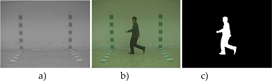
a) Background model f_b(x,y,t), b) one frame, c) object segmentation, video 019-nm-06-090 CASIA gait database

2.3. Gait Mark Location in Non-occlusion Frames

Based on the image f_g(x,y,t) and the corresponding pixel coordinates of the human silhouette, (x_s,y_s), segmented in section B, the height λ of the person is computed by [15]

λ = \max (y_{s}) - \min (y_{s})

(5)

The height is the first computation because other parameters like neck, shoulder, hip, knee and ankle row positions depend on it. Based on anatomic studies [16, 17], the estimation of the neck, shoulder, hip, knee and ankle row positions are [15, 18]

\begin{array}{l} y_{n e c k} = \min (y_{s}) + 0.13 * λ y_{s h o u l d e r} = \min (y_{s}) + 0.182 * λ \\ y_{h i p} = \min (y_{s}) + 0.50 * λ y_{k n e e} = \min (y_{s}) + 0.75 * λ \\ y_{a n k l e} = \min (y_{s}) + 0.90 * λ \end{array}

(6)

Figure 2.

Silhouette regions, b) skeletonization, video 124-nm-04-090 CASIA gait database

Base on the previous estimations the human silhouette is divided horizontally into several horizontal regions, Figure 2a. These regions are used to obtain better linearization of the skeleton model of the silhouette. The regions are defined as follows: region 1 [min(y_s), y_neck], region 2 [y_neck, y_shoulder], region 3 [y_shoulder, y_hip], region 4 [y_hip,y_knee] and region 5 [y_knee,y_ankle]. Skeletonization is achieved by applying Equation (7) to each row of the different regions [18].

x_{μ} = (x_{i} + x_{f}) / 2

(7)

The hip coordinates correspond to the midpoint of the row y_hip. For regions 1 to 3, x_i corresponds to the first column silhouette of a row y_i and x_f is the last column of y_i, such that x_μ represents the medium column in [x_i, x_f]. The regions 4 and 5 include both legs, therefore the previous methodology is applied separately to each leg. When noise is detected in the calculation of x_μ, out of a range of more than 5 pixels with respect the previous row, x_μ is adjusted to its previous value. The resulting skeleton is shown in Figure 2b.

The segments of this skeleton are used to estimate the body marks relevant to the gain analysis. These segments are determined by computing the angles of the skeleton segments θ_s [18]

θ_{s} = \tan^{- 1} ({(\sum_{r = 1}^{n} x_{r} - \bar{x})}^{2} / \sum_{r = 1}^{n} (y_{r} - \bar{y}) (x_{r} - \bar{x}))

(8)

For example θ₁ corresponds to the segment slope of the region, [min(y_s), y_neck]. The coordinates (x_r,y_r) are the positions of the non-linearized segment of the skeletons, $\bar{x}$ and $\bar{y}$ correspond to the mean values of the linear regression used to linearize the skeleton segment and n is the number of points of the segment s. Using the θ_s angles the estimation of the location, (x_p, y_p), of the gait body marks is achieved by [18]

(x_{p}, y_{p}) = [x_{p - 1} + L_{p} \cos (θ_{s}), y_{p - 1} + L_{p} \sin (θ_{s})]

(9)

Figure 3.

a) Silhouette segments, b) gait mark estimations, video 124-nm-04-090 CASIA gait database

where p = {neck, hip, knee, ankle}, (x_p-1, y_p-1) corresponds to the previous gait body mark and L_p stands for the segment length. This length is approximated considering the height of the person under analysis according to [16, 17]. This estimation is improved later and it is explained in Section J. The gait body segments, as well as the gait body marks resulting from the previous process, are illustrated in Figure 3.

2.4. Knee and Ankle Mark Location During Occlusion Frames of the Stance Limb, Initial and mid-Swing

One of the problems involved in gait body mark location and where the previous method does not work is during leg occlusion. This situation occurs in the stages of mid-stance and mid-swing. Therefore, knee and ankle detection is performed during occlusion frames as follows. The stance limb marks during occlusion are obtained from its marks prior to the occlusion. This is because the knee and ankle movements are minimal. The new knee position is calculated by

(x_{φ}, y_{φ}, t + 1) = {\begin{matrix} (x_{φ} - 1, y_{φ}, t) \begin{matrix} ​ & i f \end{matrix} \begin{matrix} ​ & ε = 1 \end{matrix} \\ (x_{φ} + 1, y_{φ}, t) \begin{matrix} ​ & i f \end{matrix} \begin{matrix} ​ & ε = 2 \end{matrix} \end{matrix}

(10)

where (x_φ,y_φ) corresponds to the previous knee position, ε is a movement direction indicator, 1 indicates a movement from right to left of the person and 2 from left to right from the camera point of view. The ankle location during the occlusion frames is considered the same as the previous position

(x_{α}, y_{α}, t + 1) = (x_{α}, y_{α}, t)

(11)

2.5. Knee and Ankle Mark Location During Occlusion Frames of the Swinging Limb, Initial Swing

The next step is to calculate the swinging limb marks during occlusion. In the CASIA database, occlusion occurs during 4 or 5 frames. The two first frames correspond to initial swing and the other frames to the mid-swing.

Figure 4.

Silhouette contour during occlusion, b) swinging limb slope, θ_β, video 124-nm-04-090 CASIA gait database

Gait mark detection of the swinging limb during the initial swing is obtained by analysis of a contour silhouette, Figure 4, as follows. A line segment is obtained by finding the rightmost points of the calf of the leg. These points are determined by analysis of the rows y_knee and y_ankle. Segment line linearization is then computed with (8) and the slope of the swinging limb is calculated.

It is important to notice that segment linearization is only computed on the maximum points of the perimeter with a negative slope because these points correspond to the calf of the leg. It can be observed in Figure 4a that the sole has a positive slope, such that using the sole point for segment linearization, the swinging limb angle will be incorrect. Considering the aforementioned issues, the swinging limb slope θ_β is calculated using (8) and then the corresponding line segment with that slope is drawn, Figure 4b. This line is displaced to the medium point of the calf of the leg area. The location of the swinging limb ankle mark is determined as point, (x_β, y_β), which is the coordinate two points before the last point over the line segment inside the silhouette. This coordinate is now used in conjunction with the calf of the leg length [16] to determine the swinging limb knee mark. The calf of the leg length is calculated by

l_{ε} = λ * 0.25

(12)

and the knee coordinate, (x_ψ, y_ψ), is the coordinate (x_k, y_k) of the n point used to compute u(k) that better approximate l_ε

u (k) = \sum_{k = 1}^{n} \sqrt{{(x_{β} - x_{k})}^{2} + {(y_{β} - y_{k})}^{2}}

(13)

Figure 5 illustrates the marks of knee and ankle in the swinging limb during occlusion.

Figure 5.

Knee and ankle mark location for initial swing during occlusion

2.6. Knee and Ankle Mark Location During Occlusion Frames of the Swinging Limb, Mid-swing

The knee and ankle location during mid-swing requires a new approach because there is a significant loss of the swinging limb information. First the ankle position is located. The ankle row y_β is determined in the interval y_ankle ± m_h, where m_h is 15 pixels in this study and it depends on the height of the persons. y_β corresponds to the row of the column, x_fr, to the far right in the interval y_ankle ± m_h inside the silhouette. The ankle column x_β will be x_fr - m_f, where m_f depends on the foot width, in this study it was considered 5 pixels. Following this stage, the knee position is determined. The row, y_ψ is calculated by determining the column of the silhouette to the far left in the interval y_knee ± m_h. The knee column will correspond to the column where y_ψ was defined plus 5 pixels. The ankle and knee positions during mid-swing are shown in Figure 6.

Figure 6.

Ankle and knee positions during mid-swing

2.7. Cycle Time

Cycle time, ρ, stands for the time elapsed between a specific gait position and the next occurrence of this position and is computed by

ρ = ς / f p s

(14)

where ζ is the number of frames elapsed for the repetition of the specific position and fps stands for frame per second. The CASIA database was acquired at 25 frames per second. In this research, the occurrence of a single limb support was considered as the initial gait position. A single limb support is considered when all the body weight is supported by only one leg. It may happen during mid-stance or mid-swing and it must occur in the first knee occlusion frame. An illustration of a cycle time is shown in Figure 7.

Figure 7.

Position representation to obtain cycle time

2.8. Step and Stride Length

A step is considered as the distance from the heel strike of the stance foot to the heel strike of the foot ending the swing. A stride is the distance of the stance foot heel strike or the heel strike of the foot ending the swing to the next occurrence of the heel strike of the corresponding foot. The step length is the distance covered by the heel strike in a single limb support in the first occlusion frame to the end of the step, Figure 7a –7b. The stride length is the distance covered from the heel strike in a single limb support to the third single limb support, Figure 7a – 7c.

2.9. Speed and Cadence

Speed is computed by [18],

ν = δ / ρ

(15)

where δ stands for length of stride. Cadence is the number of steps in a unit time and is computed through [19]

ϖ = 120 / ρ

(16)

In this research the unit time used was 120 seconds [19].

2.10. Gait Marks Adjustment

The previous section described the estimation of the main gait marks. In order to obtain a better modelling of the gait kinematic, an adjustment to the estimation marks of the hip, knee and ankle is achieved. The adjustment is performed through a local search of a better location considering the leg shape and gait cycle phase. The basic idea is to adjust a location if the estimation, for example, is too close to an edge. Due to space restriction just a brief description is provided in this paper, a complete description can be found in [20].

3. Evaluation of the Algorithm

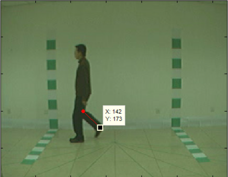
3.1. Ground Truth

The gait mark determination algorithm was evaluated against a ground truth. The ground truth was generated by manually locating the gait marks of the hip, knee and ankle as shown in Figure 8. The ground truth was obtained from three videos randomly chosen; 124-nm-06-090 frames 50 to 67, 007-nm-04-090 frames 64 to 87 and 100-nm-06-090 frames 50 to 87. One video corresponds to a man and the other two to women. Comparisons of the kinematic results of the proposed algorithm versus the ground truth are illustrated in Figures 9 - 11. The upper plots show the angles of the knee and the lower the angles of the hip. The x- axis is the number of the video frame and the y-axis is the angles of the articulation.

Figure 8.

Ground truth for a frame of video 124-nm-06-090

Quantitative results are provided in Tables 1–3. The green colour corresponds to the most forward leg.

On the one hand, the evaluation of video 124-nm, Figure 9 and Table 1, shows that the worst case occurs in hip 1 with errors greater than 5^o in 5 frames. On the other hand, positions of the knees are correctly located, as well as hip 2 in several frames. The good performance of the algorithm can also be observed since 97 of 108 frames, 89%, have differences of less than 5^o.

Figure 9.

Kinematic comparison of the proposed algorithm versus ground truth, video 124-nm-06-090

Table 1.

Kinematic performance for video 124-nm-06-090

	Frames with difference > 5°	Frames with difference < 5°	Max difference	Min difference	Difference average
Knee 1	2	25	6.7521	0.00	2.4014
Knee 2	1	26	6.4831	0.00	2.1217
Hip 1	5	22	13.5469	0.1237	3.6168
Hip 2	3	24	7.1168	0.00	2.5593

The results of video 007-nm-04-090, Figure 10 and Table 2, are not as good as for the video 124-nm-06-90, but they are still acceptable. They indicate 80% of correct detection, 76 frames out of 96 with an error less than 5^o.

Video 100-nm-04-90 presents the best results, Figure 11 and Table 3. It reaches 91%, 138 over 152 frames, of performance for differences less than 5^o. The average of the maximum differences is 6.695^o.

Figure 10.

Kinematic comparison of the proposed algorithm versus ground truth, video 007-nm-04-090

Table 2.

Kinematic performance for video 007-nm-04-090

	Frames with difference > 5°	Frames with difference < 5°	Max difference	Min difference	Difference average
Knee 1	1	23	9.5027	0.00	2.1887
Knee 2	4	20	9.8697	0.00	2.7990
Hip 1	11	13	21.2961	0.0789	5.3572
Hip 2	4	20	6.4287	0.1831	3.1569

Figure 11.

Kinematic comparison of the proposed algorithm versus ground truth, video 100-nm-04-090

Comparisons of the proposed method with the work of Yoo [18] and the medical experiments reported by Murray [21] and Kabada [22] with respect to cycle time, step and stride length and gait speed were performed in the research. These results also showed comparable findings with respect to the medical results.

Table 3.

Kinematic performance for video 100-nm-04-090

	Frames with difference > 5°	Frames with difference < 5°	Max difference	Difference average
Knee 1	0	38	4.7681	1.1942
Knee 2	1	37	6.9246	2.1320
Hip 1	4	34	7.6707	2.4405
Hip 2	9	29	7.4314	2.9452

In general and according to the previous results the proposed method to determine information of human gait kinematic provides acceptable information to be used in a powered assistance robotic mechanism. The use of this information in robotic simulation is described in the next section.

4. Kinematic analysis

We apply the DH algorithm to the legs and trunk, and only consider the sagittal plane results in the coordinate systems' assignation shown in Figure 12. The body is upright with the left leg raised to avoid overlapping of coordinate systems in the image.

The z-axes are not shown in the figure for the purposes of clarity, but they stand out from the page, defining positive angles for the counter clockwise rotation. The transformation matrix which maps the right knee with respect to the right ankle is given in Equation (17).

T_{r a}^{r k} = [\begin{matrix} \cos θ_{r a} & - \sin θ_{r a} & L_{r a} \cos θ_{r a} \\ \sin θ_{r a} & \cos θ_{r a} & L_{r a} \sin θ_{r a} \end{matrix}]

(17)

Where L_ra is the length of the calf of the leg and θ_ra is the angle of the right ankle. The transformation matrix which maps the right hip with respect to the right knee is given in Equation (18).

T_{r k}^{r h} = [\begin{matrix} \cos θ_{r k} & - \sin θ_{r k} & L_{r k} \cos θ_{r k} \\ \sin θ_{r k} & \cos θ_{r k} & L_{r k} \sin θ_{r k} \end{matrix}]

(18)

L_rk is the length of the thigh and θ_rk is the angle of the right knee. The transformation matrix which maps the shoulder with respect to the right hip is given in Equation (19).

T_{r h}^{s} = [\begin{matrix} \cos θ_{r h} & - \sin θ_{r h} & L_{r h} \cos θ_{r h} \\ \sin θ_{r h} & \cos θ_{r h} & L_{r h} \sin θ_{r h} \end{matrix}]

(19)

Figure 12.

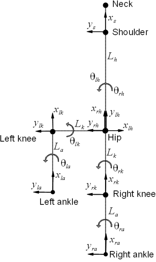
Coordinate systems' assignation

Here, L_rh is the length of the trunk and θ_rh is the angle of the right hip. Similar to the right leg, the transformation matrices for the left leg are given in Equations (20)-(21).

T_{l a}^{l k} = [\begin{matrix} \cos θ_{l a} & - \sin θ_{l a} & L_{l a} \cos θ_{l a} \\ \sin θ_{l a} & \cos θ_{l a} & L_{l a} \sin θ_{l a} \end{matrix}]

(20)

T_{l k}^{l h} = [\begin{matrix} \cos θ_{l k} & - \sin θ_{l k} & L_{l k} \cos θ_{l k} \\ \sin θ_{l k} & \cos θ_{l k} & L_{l k} \sin θ_{l k} \end{matrix}]

(21)

T_{l h}^{s} = [\begin{matrix} \cos θ_{l h} & - \sin θ_{l h} & L_{l h} \cos θ_{l h} \\ \sin θ_{l h} & \cos θ_{l h} & L_{l h} \sin θ_{l h} \end{matrix}]

(22)

Here, θ_la, θ_lk and θ_lh are the angles of the left ankle, left knee and left hip, respectively. Also, it is assumed that L_ra= L_la, L_rk= L_lk, and L_rh= L_lh.

In order to be able to simulate the motion of the body using the angles obtained from the video sequences, we need to map the swing leg with respect to the stance leg. Considering the right leg as the stance leg, we can map the left knee with respect the right ankle using Equation (23).

T_{r a}^{l k} = T_{r a}^{r k} T_{r k}^{r h} T_{r h}^{s} T_{s}^{l h} T_{l h}^{l k}

(23)

The transformation matrices T^lh_s and T^lk_lh, which map the left hip with respect to the shoulder, and the left knee with respect to the left hip, can be obtained by inverting Equations (22) and (21), respectively. In a similar way, the left ankle can be mapped using Equation (24).

T_{r a}^{l a} = T_{r a}^{l k} T_{l k}^{l a}

(24)

The transformation matrix T^la_lk can be obtained inverting Equation (20). The mapping of the left ankle with respect the right ankle starts with the toe off, through the middle swing, until the left heel lands on the floor.

Now, considering the left leg as the stance leg and the right leg as the swing leg, we need to map the right ankle with respect to the left ankle. Equation (25)

T_{l a}^{r a} = T_{l a}^{l k} T_{l k}^{l h} T_{l h}^{s} T_{s}^{r h} T_{r h}^{r k} T_{r k}^{r a}

(25)

The transformation matrices T^rh_s,T^rk_rh and T^ra_rk can be obtained by inverting Equations (19)–(17), respectively.

Equations (17)–(22) are consistent with Equation (9) for the determination of the knee, hip and shoulder positions for both legs, with respect to the previous body mark. Now we need to link or relate the definition of the hip, knee and ankle angles with the definition of the angles in Figure 12. The angle of the knee is defined with respect to the vertical and is measured with an absolute value as shown in Figure 13. The angle of the hip is measured with respect to vertical, also as shown in Figure 13. Considering the right leg as the stance leg, we can calculate the angle of the stance (right) knee using Equation (26).

θ_{s k} = | θ_{r a} |

(26)

The angle of the swinging (left) knee can be calculated using Equation (27).

θ_{s w k} = | θ_{r a} + θ_{r k} + θ_{r h} - θ_{l h} - θ_{l k} |

(27)

Figure 13.

Definition of the knee and hip angles

Considering the walking simulation of the system in Figure 12, shown in Figure 14, and using the values for θ_ra, θ_rk, θ_rh, θ_la, θ_lk and θ_lh, used for this simulation, we can apply Equations (26) and (27) to obtain the values for the right knee as defined in Figure 13. Figure 15 shows the plot of the knee angles.

Comparing the upper left plot in Figure 9, we can see a very good approximation of the knee angle pattern. The angle of the hip can be calculated in a similar way to that used for the knee.

5. Results and conclusions

This paper presented an automatic visual gait analysis method able to detect hip, knee and ankle positions in the different gait phases, as well as gait cycle analysis, cycle time, step and stride length, speed and cadence. The proposed method was also able to deal with the occlusion situations that occur in the stages of mid-stance and mid-swing. The visual gait analysis method, besides being an automatic method, shows acceptable results compared with the manual ground truth as demonstrated in section III. Quantitative results indicate 86.66% of correct detection for the thigh and knee angles with values less than 5^o. A kinematic analysis was also completed obtaining the equations to map the main body marks with respect to the stance ankle. Simulation results present a very good approximation of the knee angle pattern compared with the data obtained in the gait analysis part. In addition, some equations are given to relate to the medical definition of the limbs' angles with the definition given by the coordinate systems' assignation using the DH algorithm.

Figure 14.

A simulation of a walking pattern

Figure 15.

Angle of the knee as defined in Figure 13

Footnotes

6. Acknowledgments

The authors thank Fondo Mixto de Fomento a la Investigación Científica y Tecnológica CONACYT- Gobierno del Estado de Chihuahua for supporting this research under grant CHIH-2009-C02-125358. Portions of the research in this paper use the CASIA Gait Database collected by Institute of Automation, Chinese Academy of Sciences.

References

Dollar

A.M.

Herr

, “Lower Extremity Exoskeletons and Active Orthoses: Challenges and State-of-the-Art” IEEE Transactions on Robotics, vol. 24, No. 1, pp 1–15, February 2008.

Kawamoto

Sankai

, “Power Assist Method Based on Phase Sequence Driven by Interaction between Human and Robot Suit” Proceedings of the 2004 IEEE International Workshop on Robot and Human Interactive Communication Kurashiki, Okayama Japan, pp 491–496, September, 2004.

Kazerooni

Steger

R. R.

, “The Berkely Lower Extremity Exoskeleton” Transaction of the ASME, vol. 128, no. 3, pp 14–25, March 2006.

Mündermann

Corazza

Andriacchi

, “The evolution of methods for the capture of human movement leading to markerless motion capture for biomechanical applications” Journal of NeuroEngineering and Rehabilitation, vol. 3, no. 6, pp. 2–11, March 2006.

Perry

, Gait Analysis: Normal and Pathological Function NJ: Slack, 1992.

Senanayake

C.M.

Senanayake

S.M.N.A.

, “Computational Intelligent Gait-Phase Detection System to Identify Pathological Gait” Information Technology in Biomedicine, IEEE Transactions on, vol. 14, no. 5, pp. 1173–1179, September 2010.

Cardenas-Maciel

S. L.

Castillo

Aguilar

L.T.

, “Generation of walking periodic motions for a biped robot via genetic algorithms” Appl. Soft Comput. 11(8): 5306–5314, 2011.

Cardenas-Maciel

S. L.

Castillo

Aguilar

L. T.

Castro

J. R.

, “A T-S Fuzzy Logic Controller for biped robot walking based on adaptive network fuzzy inference system” Proceeding of the IJCNN 2010, pp1–8.

Porta-García

M. A.

Montiel

Castillo

Sepulveda

, “Optimal Path Planning for Autonomous Mobile Robot Navigation Using Ant Colony Optimization and a Fuzzy Cost Function” Evaluation. Analysis and Design of Intelligent Systems Using Soft Computing Techniques, vol. 41/2007, pp 790–798, 2007.

10.

Lauer

R.T.

Smith

B.T.

Betz

R.R.

, “Application of a neuro-fuzzy network for gait event detection using electromyography in the child with Cerebral palsy” Biomedical Engineering, IEEE Transactions on, vol. 52, no. 9, pp. 1532–1540, September 2005.

11.

Stefanovic

, “A portable measurement system for the evaluation of human gait” Journal of Automatic Control, vol. 19, no. 1, pp. 1–6, 2009.

12.

Huang

Chen

Shi

, “Gait Event Detection with Intelligent Shoes” in Information Acquisition, 2007. ICIA '07. International Conference on, 2007, pp. 579–584.

13.

Center of biometrics and security research. [Online](2012), Available http://www.cbsr.ia.ac.cn/english/Gait%20Databases.asp

14.

Al-Khateeb

Petrou

, “Automatic change detection in an indoor environment” in Computer Vision and Pattern Recognition Workshops (CVPRW), 2010 IEEE Computer Society Conference on, San Francisco, CA, 2010, pp. 53–58.

15.

Goffredo

Bouchrika

Carter

J.N.

Nixon

M.S.

, “Self-Calibrating View-Invariant Gait Biometrics” Systems, Man, and Cybernetics, Part B: Cybernetics, IEEE Transactions on, vol. 40, no. 4, pp. 997–1008, August 2010.

16.

Dempster

W. T.

Gaughran

G. R. L.

, “Properties of body segments based on size and weight,” Amer. J. Anatomy, vol. 120, no. 1, pp. 33–54, Jan. 1965.

17.

Drillis

Contini

, “Body Segment Parameters” Technical Report 1163–03, New York University, New York, 1966.

18.

Yoo

Nixon

M.S.

, “Automated Markerless Analysis of Human Gait Motion for Recognition and Classification” ETRI Journal, vol. 33, no. 2, pp. 259–266, April 2011.

19.

Whittle

M.W.

, Gait Analysis: An Introduction, 4th ed.: Elsevier, 2007, New York.

20.

Arias

, “Human Gait Analysis Based on 2D/Kinect Visual Perception and Its Clinic Diagnosis Using fuzzy Systems,” Master Thesis, July 2012.

21.

Murray

M.P.

Drought

A.B.

Kory

R.C.

, “Walking Patterns of Normal Men” J. Bone and Joint Surgery, vol. 46A, no. 2, pp. 335–360, March 1964.

22.

Kadaba

M. P.

Ramakrishnan

H. K.

Wootten

M. E.

, “Measurement of Lower Extremity Kinematics During Level Walking” Journal of Orthopaedic Research, vol. 8, no. 3, pp. 383–392, May 1990.