Image Jacobian Matrix Estimation Based on Online Support Vector Regression

Abstract

Research into robotics visual servoing is an important area in the field of robotics. It has proven difficult to achieve successful results for machine vision and robotics in unstructured environments without using any a priori camera or kinematic models. In uncalibrated visual servoing, image Jacobian matrix estimation methods can be divided into two groups: the online method and the offline method. The offline method is not appropriate for most natural environments. The online method is robust but rough. Moreover, if the images feature configuration changes, it needs to restart the approximating procedure. A novel approach based on an online support vector regression (OL-SVR) algorithm is proposed which overcomes the drawbacks and combines the virtues just mentioned.

Keywords

Image Jacobian matrix visual servoing online support vector regression (OL-SVR)

1. Introduction

Visual servoing has become a very popular field of research. The scheme is usually divided into two categories: position-based and image-based[1]. With position-based systems, the manipulator is moved after the calculation of the end-effector pose in the workspace coordinates; the image features are used for fitting a geometric model of the target to estimate the relative pose of the target with respect to the end-effector. Image-based systems are also called feature-based systems – the error signal is defined in terms of image features and, therefore, it is directly measured in the image coordinate. Therefore, any computational costs are significantly reduced and the system becomes less sensitive to errors in camera calibration and system modelling. As this relationship is nonlinear and its parameters are strongly correlated, it presents a significant challenge to control and design and has proven to be difficult to analyse theoretically. Pioneering work in the field of image-based visual servoing stems from Weiss [2]. In contrast with position-based visual servoing methods, image-based visual servoing does not require such computationally complex depth estimation nor inaccurate sensor calibration. On the other hand, it is necessary to provide some other information about the 3D structure of the object in the camera frame. It is possible to combine the advantages of the two schemes by dynamically switching between them. Malis et al. adopt hybrid state vectors composed by both 2D and 3D visual measurements, referred to as 2.5D visual servoing [3, 4].

However, in order to move the robot end-effector to the desired position using visual information, some priori knowledge – such as the camera model, kinematics and robot dynamics – may be necessary. A correct estimation of the pose is crucial with the position-based method and coarse estimations will thus induce perturbations on the realized trajectory as well as affecting the accuracy of the pose reached after convergence. However, for image-based method, misestimation can thus cause the system to become unstable and rough estimations will only imply perturbations in the trajectory performed by the robot in reaching its desired pose, though they will have no effect on the accuracy of the pose reached. The most important scheme of the image-based method is directly associates the pose error of the end-effector with an image Jacobian matrix. This matrix models the variation of selected image features with respect to the difference of the current end-effector pose from its nominal pose. By solving the inverse problem, it is possible to calculate the desired end-effector pose from the differences in the image feature vector. Due to the inherent nonlinearity in a camera-robot system, the Jacobian matrix involves inaccurate camera parameters and unknown depths of image features.

One way to overcome the above difficulties is to identify or calibrate the robot and camera parameters. Reference [5] gives a comprehensive survey of camera self-calibration techniques. However, it would be a time-consuming task.

The offline learning method, led by neural networks-based visual servoing, has been a growing research area, whereby the neural networks approximate the inverse image Jacobian, relating change in image features to change in robot position. The key attribute of neural networks is their ability to serve as a general nonlinear model. Thousands of data points are fed through a black box until the output of the network converges into the true system. It has been shown that any function of practicable interest can be closely approximated arbitrarily with a neural network having enough neurons, at least one hidden layer and an appropriate set of weights. The high computation speed and general modelling capability of neural networks are very attractive properties for nonlinear compensation problems, as indeed robot control problems are. Hashimoto et al. utilized two BP networks – one global and one local – to approximate the Jacobian mapping [6, 7]; Kuhn et al. used an adaptive linear (ADALINE) network to approximate the inverse image Jacobian and a self-organizing map (SOM) network to select the ADALINE matrix [8]. However, the significance of visual servoing is its flexibility, but the nature of offline learning critically weakens this advantage. Besides this, the learned neural network is trained for a particular camera-robot configuration. Once this changes, retraining is generally required, which is normal in a natural environment.

Thus, a degree of adaptive visual servoing is proposed in order to improve flexibility and adaptability – from a task-oriented point of view – where online identification and control are performed simultaneously so as to avoid tedious offline calibration. To control a vision-guided robot with less prior knowledge, model-independent visual-servoing schemes are proposed [9 -14], where the camera-robot model is approximated by a linearized affine model and the Jacobian matrixes are identified online. A lot of authors have shown how the image Jacobian matrix itself can be estimated online from the measurements of robot and image motions. However, the estimated image Jacobian may deteriorate and the control may also face the singularity problem. To alleviate this, either prior knowledge is required to restrict the estimated Jacobian close to the true image Jacobian [9, 12] or else additional probing movement is needed to provide sufficient excitation for identification [10]. Yoshimi and Allen proposed an estimator of the image Jacobian for a plug-in-hole alignment task [10]. Hosada and Asada designed an online algorithm to estimate the image Jacobian [12]. Jagersand took the approach of a nonlinear least-squares optimization method using a trust-region method and Broyden estimation [11]. Piepermeier developed a dynamic Broyden Jacobian estimation for a moving target, where a stationary camera was used within the workspace [9]. Goncalves et al. proposed an online fuzzy learning method to estimate the Jacobian [15]. The input-output data was partitioned using unsupervised clustering methods and the result was used as a supervisor for fuzzy learning in a second phase.

Our task is to build a system for robot control that is independent of camera calibration and which achieves comparable regression precision of nonlinear approximation as offline methods. An online support vector regression is introduced serving as an image Jacobian matrix estimator, similar technology to which – a support vector machine (SVM) – has been frequently used in target recognition in visual servoing [13, 14]. Furthermore, we propose an adaptive switching scheme between the training procedure and the estimation procedure. Our proposed method is compared with the Broyden algorithm for visual servoing, as developed by Jagersand [11].

This paper is organized as follows. In Section 2 we recall the perspective projection model and the control scheme. In Section 3 we introduce the online support vector regression (OL-SVR). Section 4 discusses the integration of OL-SVR in a visual servoing loop. The experimenta results and discussion are presented in Section 5. Finally, Section 6 summarizes the paper.

2. Image Jacobian Matrix Estimation

The objective of visual servoing is to move the robot tip of a robotic manipulator towards a target point. Dynamic control systems use a hierarchical structure: the robot is internally stabilized with the help of a second control loop which employs encoder feedback from the robot's internal joint angle sensors. This separation of the visual controller from the robot kinematics and dynamics permits a conception of the robot as an ideal Cartesian motion device which is not affected by such problems as oscillations or singularities. In other words, the visual controller can assume idealized axis dynamics because of the high sampling rates of the internal feedback loop. This simplifies the control design problem considerably. Since many robots provide an interface for Cartesian inputs or else incremental position commands, implementation is simple and portable.

In the filed of computer vision, an image feature is a real-valued quantity associated to a geometric primitive (for example, the coordinates of a point, the area of an ellipse, the angular coefficient of a line, etc.) in the image plane.

Given a vector of image features f = [f₁ … f_k] ^T ∈ ℝ ^k , the velocity twist ṙ = [v_c,w_c] ^T of the camera is mapped to ḟ by a k × 6 matrix J_image(r) called the image Jacobian matrix (or interaction matrix):

\dot{f} = J_{i m a g e} (r) \cdot \dot{r}

(1)

J_{i m a g e} (r) = (\frac{\partial f}{\partial r}) = (\begin{matrix} \frac{\partial f_{1} (r)}{\partial r_{1}} & \dots & \frac{\partial f_{1} (r)}{\partial r_{6}} \\ ⋮ & ⋱ & ⋮ \\ \frac{\partial f_{k} (r)}{r_{1}} & \dots & \frac{\partial f_{k} (r)}{r_{6}} \end{matrix})

(2)

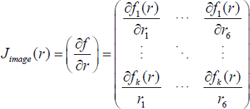
It is possible to determine the image Jacobian matrix for many features of interest. Though the following discussion is based on point features, the approach proposed in the paper can be easily extended to other features.

Given the coordinates P with homogeneous coordinates P = [x y z 1] ^T , its projection on the image plane is a 2D point with homogeneous normalized coordinates p̄ = [ū v̄ 1] ^T = [x/z y/z 1]. The corresponding coordinates in pixels are denoted as p˜ = [ũ v˜ 1] = Ap̄, where A is a non-singular matrix containing the camera intrinsic parameters:

A = [\begin{matrix} λ & 0 & u_{0} \\ 0 & λ & v_{0} \\ 0 & 0 & 1 \end{matrix}]

(3)

Here, [u₀ v₀] ^T are the coordinates of the principal point (in pixels) and λ is the focal length in pixels. If the matrix A is known, the camera is calibrated. However, to obtain a relationship which can be also used in the case of a partially uncalibrated camera, it is usually assumed that the values of [u₀ v₀] ^T are known. Hence, by defining f_u = ũ – u₀ and f_v = v˜ – v₀, the relationship is formed:

[\begin{matrix} {\dot{f}}_{u} \\ {\dot{f}}_{v} \end{matrix}] = [\begin{matrix} - \frac{λ}{z} & 0 & \frac{f_{u}}{z} & \frac{f_{u} f_{v}}{λ} & - (λ + \frac{f_{u}^{2}}{λ}) & f_{v} \\ 0 & - \frac{λ}{z} & \frac{f_{y}}{z} & λ + \frac{f_{v}^{2}}{λ} & - \frac{f_{u} f_{v}}{λ} & - f_{u} \end{matrix}] [\begin{matrix} v_{c} \\ w_{c} \end{matrix}]

(4)

The image Jacobian matrix is referred to as the image Jacobian matrix of a point feature. Obviously it is a nonlinear map between the moving frame and the robot's tip coordinates in the camera image.

Since many robots provide an interface for joint velocity inputs, most IBVS control strategies with offline training are based on the relation of the robot's joint velocity and the image feature. the form is:

\dot{f} = J_{i m a g e} \cdot \dot{r} = J_{i m a g e} \cdot J_{r o b o t} \cdot \dot{q}

(5)

where q̇ is the joint velocity input and J_robot is the relationship between the velocity in the robot's joint space and the velocity of its end-effector, i.e., the robot Jacobian matrix.

The inverse form of Eq. (5) in terms of the desired feature velocity is used as the control scheme and learning algorithm:

\dot{q} = H \cdot \dot{f}

(6)

where H is usually the pseudo-inverse of J_image · J_robot.

It is worth noting that for such systems, the joint velocities are actually dependent on the feature configuration. Take pseudo-inverse calculation-based methods, for instance – the joint velocities couple with all the features. Once the configuration changes, the learning machine needs to be retrained. Hence, the advantage of nonlinear approximating accuracy of offline learning is significantly reduced. Besides this, the inverse kinematic problem does not usually have a unique solution. Several joint positions may provide an identical end-effector position and thus the result will be unstable.

But note that the image Jacobian matrix itself of each feature is obviously independent of the feature configuration and only related to f˜_u, f˜_v, λ and Z. The first two parameters are known and λ is constant. According to Reference [16], the depth Z can be well estimated from the feature differentiation and end-effector velocity of only one point. As such, in this paper we directly estimate the image Jacobian matrix J_i for each feature.

3. Online Support Vector Regression

In recent years, the online learning-based method on the incremental version of the classical learning machine has been significantly developed. In this, a sequential data treatment is preferred – e.g., in tracking applications or time series analysis. For such applications, it is desirable that a new sample is added to or removed from the training set each time. Retraining from scratch for each new data point can be very time-consuming. Compared with batch (offline) learning methods in which data is available and simultaneously processable, incremental methods have to deal with sequentially arriving data, of which the order and quantity can be arbitrary. In general, these methods have certain advantages compared to offline methods. If there are only a few labelled samples known before-hand, we can begin learning immediately and do not have to wait for further samples.

Several incremental learning methods have been proposed, extending classical and state-of-the art offline methods. Incremental learning methods in general show comparable performances with their batch version when there is no change in the data distribution over time. The most recent methods vary from on-line discriminative kernel density estimation [17] and on-line random forests (ORF) [18] to incremental support vector machines [19, 20]. Compared with their batch learning versions, the incremental methods provide reliable results regardless of the complexity of the data distribution.

Similarly, online support vector regression (OL-SVR) is a continuous-valued function for data in a manner that shares many of the advantages of support vector regression (SVR) classification. The support vector machine was first presented in [21] and a widely-used version was proposed in [22].

In this paper, an OL-SVR algorithm is used to constitute, memorize and retrieve the image Jacobian matrix. As discussed in Section 2, the image Jacobian matrix is related to f_u, f_v, λ and Z. The image feature for each point [f_u f_v] ^T is known. The λ and Z can be calculated from end-effector velocity ṙ = [v_c w_c] ^T and feature velocity [ḟ_u ḟ_v] ^T . As such, the parameter listed above is used as the input. We rewrite the input vector x_i = [v_c w_c f_u f_v ḟ_u ḟ_v] ^T and the output vector Y_i, which contains the 12 elements [y_i¹ ··· y_i¹²] within it.

For one element y_i of the output vector, the estimation is obtained as:

f (x_{i}) = w φ (x_{i}) + b

(7)

where w is a weight vector, φ(·) is a nonlinear mapping from input space to some high-dimensional feature space, and b is a scalar representing the bias. In order to perform the estimation w of b, the SVR framework based on the ε -insensitive loss function is adopted. By introducing slack variables ξ _i and ξ _i * and quantifying estimation errors greater than ε, the estimation task can be formulated as a constrained optimization problem that minimizes the regularized loss:

\frac{1}{2} w^{T} w + C \sum_{i = 1}^{t} (ξ_{i} + ξ_{i}^{*})

(8)

subject to:

\begin{array}{l} - y_{i} + (w^{T} φ (x_{i}) + b) + ε + ξ_{i} \geq 0 \\ y_{i} - (w^{T} φ (x_{i}) + b) + ε + ξ_{i}^{*} \geq 0 \\ ξ_{i}, ξ_{i}^{*} \geq 0 \end{array}

(9)

for i = 1 ··· t, where the slack variables ξ _i and ξ _i * correspond to the size of this excess deviation for positive and negative deviations, respectively. A penalization on the norm of the weights has been imposed and is controlled by the parameter C. This primal optimization problem is transformed due to its dual quadratic optimization problem. Next, the solution to the resulting optimization problem can be expressed as:

f (x) = \sum_{i = 1}^{t} θ_{i} K (x_{i}, x)

(10)

where θ _i is defined in terms of the dual variables and K(•,•) is a kernel function. Though a Gaussian kernel is more common, a polynomial kernel is more effective with smaller hyperparameters. The objective is to minimize (8) incrementally without having to retrain the model entirely at each time point.

The first term in (2), w^Tw is the regularized term; thus, it controls the function capacity. The second term $\sum_{i = 1}^{t} (ξ_{i}^{*} + ξ_{i})$ is the empirical error measured by the S-insensitive loss function.

By Introducing Lagrange multipliers α, α*, η, η*, δ, δ*, u and u*, the KKT conditions are given without improvement:

\begin{array}{l} \frac{\partial L_{D}}{\partial α_{i}} = \sum_{j = 1}^{t} Q_{i j} (α_{j} - α_{j}^{*}) + ε - y_{i} \\ + ξ - δ_{i} + u_{i} = 0 \\ \frac{\partial L_{D}}{\partial α_{i}^{*}} = - \sum_{j = 1}^{t} Q_{i j} (α_{j} - α_{j}^{*}) + ε + y_{i} \\ - ξ - δ_{i}^{*} + u_{i}^{*} = 0 \\ δ_{i}^{(*)} \geq 0, δ_{i}^{(*)} α_{i}^{(*)} = 0 \\ u_{i}^{(*)} \geq 0, u_{i}^{(*)} (α_{i}^{(*)} - C) = 0 \end{array}

(11)

where ξ in Eq. (11) is equal to b in Eq. (7) at optimality. At most one of α and α will be nonzero and both are nonnegative. Therefore, a coefficient difference θ _i was defined as:

θ_{i} = α_{i} - α_{i}^{*}

(12)

where θ _i determines both α and α*. In addition, a margin function h(x_i) is defined as:

h (x_{i}) = f (x_{i}) - y_{i} = \sum_{j = 1}^{t} Q_{i j} θ_{j} - y_{i} + b

(13)

The OL-SVR can be obtained by first classifying all of the training points into three distinct auxiliary sets according to the KKT conditions that define the current optimal solution. Specifically, after defining the margin function h_i(x_i) as the difference f(x_i) – y_i for all time points i = 1, ···, t, the KKT conditions are expressed in terms of θ_i, h_i(x_i), ε and C. Accordingly, each data point falls into one of the following sets:

\begin{array}{l} S = {i | (θ_{i} \in [0, + C] \land h_{i} (x_{i}) = - ε) \\ \lor (θ_{i} \in [- C, 0] \land h_{i} (x_{i}) = + ε)} \\ E = {i | (θ_{i} = - C \land h_{i} (x_{i}) \geq + ε) \\ \lor (θ_{i} = + C \land h_{i} (x_{i}) \leq - ε)} \\ R = {i | θ_{i} = 0 \land | h_{i} (x_{i}) | \leq ε)} \end{array}

(14)

Set S contains the support vectors – i.e., the data points contributing to the current solution – whereas the points that do not contribute are contained in R. All error points are in E. When a new data point arrives, the incremental algorithm re-labels all of the points in an iterative way until optimality is reached again. Similarly, old data points can be discarded easily without having to retrain the machine. The algorithm details can be found in Reference [22].

4. Adaptive Switching Visual Servoing

There remain certain issues whereby if the training is online, then where do the training samples come from? Goncalves et al. used unsupervised clustering methods as a supervisor for the latter fuzzy method [15]. However, unsupervised clustering is always slow and affected by the initial clustering centre. As such, an adaptive switching scheme is proposed to solve the problem, which combines a Broyden estimator as a supervisor. The blocks of the learning process and the execution process are shown in Figure 1

Figure 1.

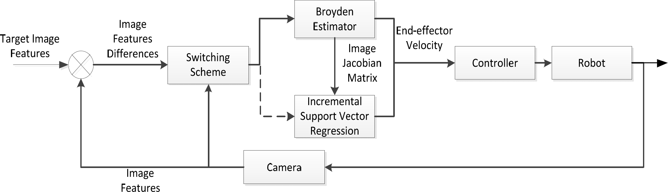
Learning and the execution process

The visual servoing begins with Broyden estimator. The input for the Broyden estimator is the last estimated image Jacobian matrix Ĵ_i–1, the move of the end-effector Δx˜_i and the observed differential of all image features Δy˜_i. Accordingly, the new image Jacobian matrix is:

{\hat{J}}_{i} = {\hat{J}}_{i - 1} + \frac{(Δ {\tilde{y}}_{i} - {\hat{J}}_{i - 1} Δ {\tilde{x}}_{i}) Δ {\tilde{x}}^{T}}{Δ {\tilde{x}}_{i}^{T} Δ {\tilde{x}}_{i}}

(15)

The new image Jacobian matrix Ĵ_i is used to inversely calculate the desired velocity by Eq. (6). Simultaneously, the Ĵ_i is divided into m submatrices [Ĵ_i¹ ··· Ĵ_i^m] ^T , one for each point. The submatrix Ĵ_i^m is the training output, and the corresponding training input is x_i^m = [v_c w_c f_u^m f_v^m ḟ_u^m ḟ_v^m] ^T . The socalled “virgin” learning did not always find a satisfying fit through the OL-SVR until the switching condition was satisfied:

\frac{‖ J_{i}^{B r o y d e n} - J_{i}^{I S V R} ‖}{‖ J_{i}^{B r o y d e n} ‖} < σ for i = t - l + 1, \dots t

(16)

where σ is the error tolerance limit, t is the current time and l is a length which defines how many samples need to be compared. σ is 0.01 or 0.001 in common, and l is set manually. Afterwards, the visual servoing system will switch to OL-SVR.

However, better results are given when using more targets, and so the training does not stop after switching. The only difference between before and after training is that the image Jacobian matrix Ĵ_image used in Eq. (6) is taken directly from OL-SVR rather than from Broyden. The OL-SVR will provide a reasonably accurate estimation, even soon after changing the image feature configuration, while Broyden estimation is usually very rough at that point. This is hardly a concern in relation to the over fitting problem of large scale training owing to the inherent advantages of SVR.

5. Experiment

The work presented in this paper is compared with the known Broyden method. The simulation results for a robotic manipulator with six degrees of freedom are shown in this section. The simulation platform is the toolbox provided by Corke [23]. The experimental task is that of moving a camera to a specific pose so that the image in the camera matches the target image. The image features consist of four points. The initial position of the camera is set randomly within an acceptable limit. When the OL-SVR is learned, it can be used instead of the Broyden estimator.

Figures 2–3 illustrate a complete learning procedure and the red line indicates the switching moment. Figure 2 shows the variation of error, which is defined in Eq. (13), σ is 0.01 and l is 20. Every interval between a peak and a valley is a dependant visual servoing task. The inaccurate initial values of the Broyden method cause these peaks and so the switching condition is always satisfied in the valley period of a task. The data shows an overall decline in the error before switching, which means that the image Jacobian matrix predicted by OL-SVR converges with that of Broyden's. After switching to OL-SVR, and because the visual servoing is driven by the image Jacobian matrix predicted by OL-SVR, the variation of error lowers and remains stable. Figure 3 illustrates the variation of the feature error (an average of four points). After switching, the feature error declines faster than before, which can be seen more clearly in Figures 4–5.

Figure 2.

Error of the Image Jacobian Matrix

Figure 3.

Average Feature Error

Figure 4.

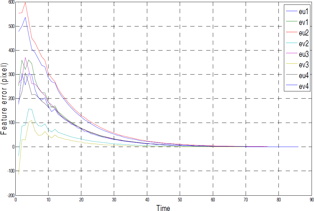
Error of the image feature in the Broyden method

Figure 5.

Error of the image feature in the proposed method

Figures 4 -9 illustrate the comparison of the experimental results for visual servoing obtained by the Broyden method and the proposed method (after switching) for the same task. Before switching, the effect of the proposed method is the same as the Broyden method, and so the comparison of the experimental results between the Broyden method and the proposed method (before switching) is not provided in the following.

Figure 6.

End-effector velocity in the Broyden method

Figure 7.

End-effector velocity in the proposed method

Figure 8.

Points trajectories in Broyden method

Figure 9.

Points trajectories in the proposed method

Figures 4–5 show the experimental results for u and v feature errors. It demonstrates that the error in the proposed method declines more smoothly than the Broyden method. This conclusion can also be drawn from Figures 8–9. Since in the proposed method the OL-SVR is well trained, this means that the image Jacobian matrix is “known”. Accordingly, the perturbations in the initial phase of the Broyden method hardly appear in the proposed method. Besides this, the proposed method has a higher convergence rate. The error in the proposed method declines to 50% at the 10th step while the Broyden method reaches this at the 20th step.

Figure 6 more clearly reveals the reason why the error changing is rough in the Broyden method. The calculated velocity changes drastically and some DOFs generate unnecessary movement.

In Figures 8–9, it is clear that the path of the proposed method is closer to the ideal path, while the path calculated by the Broyden method contains some unexpected motions.

However, a limitation of the proposed method is that the parameters used in OL-SVR are set manually while the training performance relies on choice. This is also the main problem for other applications based on the SVM/SVR technique. Fortunately, the proposed method directly estimates the image Jacobian matrix, which is a low-order model. As such, the influence is not very strong which means that a bad choice affects the training time more than the final accuracy. This leads to the other problem: the training time. Although online methods have significantly decreased the training time for one increment/decrement compared with the offline methods, the training samples increase and so the time consumption becomes considerable, especially for high-speed processing situations. All that can be done is to wait for further developments in the implementation of the OL-SVR algorithm. This last, minor problem is the switching condition. For some concentrated samples, the switching condition will be satisfied very quickly but the adaptability of a trained model this is unsatisfactory. A task deviating from the known samples will not be handled well. However, since such learning does not stop after switching, the data from this task will be learned by OL-SVR to provide better results for the latter task. The generalization of SVR can also reduce the problem somewhat.

6. Conclusion

Motivated by the need for fast online model learning in robotics, this paper describes a form of visual servoing control of robot manipulators based on online support vector regression. The regression machine is used to estimate the image Jacobian matrix instead of the joint (or end-effector) velocity, which avoids the dependence problem of a particular feature configuration. An adaptive switch scheme is implemented which integrates a Broyden estimator as a supervisor for the training for OL-SVR. The proposed approach provides more precise results for visual serving micromanipulation. The validity is confirmed by experiment, the results of which achieve the desirable effects.

Footnotes

7. Acknowledgments

This work is supported by the National High Technology Research and Development Programme 863 of China (Grant No. 2008AA8041302), the Natural Science Foundation of China (Grant No. 60873032) and the Doctoral Programme Foundation of Ministry of Education of China (Grant No. 20100142110020). The authors thank the anonymous reviewers and the editors for their many helpful suggestions.

References

Chaumette

and Hutchinson

(2006) Visual servo control – Part I: Basic approaches. IEEE Robotics & Automation Magazine. 13: 82–90.

Weiss

Sanderson

, and Neuman

(1987) Dynamic sensor-based control of robots with visual feedback. Robotics and Automation, IEEE Journal of. 3: 404–417.

Malis

Chaumette

, and Boudet

(1999) 2-1/2-D visual servoing. IEEE Transactions on Robotics and Automation. 15: 238–250.

Malis

and Chaumette

(2000) 2-1/2-D visual servoing with respect to unknown objects through a new estimation scheme of camera displacement. International Journal of Computer Vision. 37: 79–97.

Hemayed

E.E.

(2003) A survey of camera self-calibration. in Proceedings. IEEE Conference on Advanced Video and Signal Based Surveillance 2003 Miami, USA: IEEE. p: 351–357.

Hashimoto

. (1991) Self-organizing visual servo system based on neural networks. in American Control Conference, 1991. IEEE. p: 2262–2267.

Hashimoto

. (1992) Visual control of robotic manipulator based on neural networks. Industrial Electronics, IEEE Transactions on. 39: 490–496.

Kuhn

Buessler

, and Urban

(1995) Neural approach to visual servoing for robotic hand eye coordination. in Neural Networks, 1995. Proceedings., IEEE International Conference on. IEEE. p: 2364–2369.

Piepmeier

J.A.

McMurray

G.V.

, and Lipkin

(2004) Uncalibrated dynamic visual servoing. IEEE Transactions on Robotics and Automation. 20: 143–147.

10.

Yoshimi

B.H.

and Allen

P.K.

(1995) Alignment using an uncalibrated camera system. Robotics and Automation, IEEE Transactions on. 11: 516–521.

11.

Jägersand

and Nelson

(1996) On-line estimation of visual-motor models using active vision. image. 11: 1.

12.

Hosoda

and Asada

(1994) Versatile visual servoing without knowledge of true Jacobian. IEEE. p: 186–193 Intelligent Robots and Systems '94. ‘Advanced Robotic Systems and the Real World’, IROS '94. Proceedings of the IEEE/RSJ/GI International Conference on.

13.

Zeng

X.J.

Huang

X.H.

, and Wang

(2009) The Improved SVM Multi Objects' Identification For the Uncalibrated Visual Servoing. International Journal of Advanced Robotic Systems. 6: 59–66.

14.

Huang

X.H.

Zeng

X.J.

, and Wang

(2010) The Uncalibrated Microscope Visual Servoing for Micromanipulation Robotic System. In: Fung

R.-F.

, editor. Visual Servoing. InTech: P. 53–76.

15.

Goncalves

and Torres

(2010) Learning Approaches to Visual Control of Robotic Manipulators. in COGNITIVE 2010, The Second International Conference on Advanced Cognitive Technologies and Applications. p: 103–108.

16.

De Luca

Oriolo

, and Giordano

P.R.

(2008) Feature depth observation for image-based visual servoing: Theory and experiments. International Journal of Robotics Research. 27: 1093–1116.

17.

Kristan

and Leonardis

(2010) Online discriminative kernel density estimation. in 2010 20th International Conference on Pattern Recognition, ICPR 2010. Istanbul, Turkey: IEEE. p: 581–584.

18.

Kalal

. (2010) P-N Learning: Bootstrapping Binary Classifiers by Structural Constraints. in 2010 IEEE Conference on Computer Vision and Pattern Recognition. Los Alamitos: IEEE Computer Soc. p: 49–56.

19.

Cauwenberghs

and Poggio

(2001) Incremental and decremental support vector machine learning. Advances in neural information processing systems. p: 409–415.

20.

Ralaivola

and d'Alche-Buc

(2001) Incremental support vector machine learning: A local approach. in International Conference on Artificial Neural Networks (ICANN 2001). Vienna, Austria: Springer-Verlag. p: 322–330.

21.

Martin

(2002) On-line support vector machine regression. in 13th European Conference on Machine Learning. Helsinki, Finland. p: 282–294.

22.

J.S.

Theiler

, and Perkins

(2003) Accurate on-line support vector regression. Neural Computation. 15: 2683–2703.

23.

Corke

P.I.

, Robotics, Vision & Control2011, Berlin: Springer. p: 558.