Robust Corner Detection by Image-Based Direct Curvature Field Estimation for Mobile Robot Navigation

Abstract

In this paper, a novel corner detection method is presented, to extract geometrically important corners for robot applications, such as indoor mobile robot navigation or manipulation. Intensity-based corner detectors, such as the Harris corner, can detect corners in noisy environments, but have inaccurate corner positions and miss the corners of obtuse angles. Edge-based corner detectors, such as the Curvature Scale Space, can detect structural corners, but show unstable corner detection due to incomplete edge detection in noisy environments. The proposed image-based direct curvature estimation can overcome limitations in both the inaccurate structural corner detection of the Harris corner detector (intensity-based) and the unstable corner detection of the Curvature Scale Space, caused by incomplete edge detection. Various experimental results validate the robustness of the proposed method.

Keywords

Corner detection intensity-based contour-based orientation field curvature field

1. Introduction

An interest point is one that has a location in space, but no spatial extent. The presence of interest points can drastically reduce the required computation time. As such, these points are frequently used to compensate for many vision problems, such as camera calibration, 3D reconstruction, stereo matching, image registration, structure from motion, image mosaicing, motion tracking, object recognition and mobile robot navigation [17]. We are specifically focusing on feature extraction for robot applications, such as indoor mobile robot navigation [21] and manipulation [23]. Many different interest point detectors have been proposed with a wide range of definitions. Some detectors find points of high local symmetry [9, 12], whereas others locate corner points. Corner points are more frequently used to solve correspondence problems, as they are formed from two or more edges that define the boundary between different objects or parts of the same object.

Corner detectors have to satisfy several criteria as shown in Figure 1. First, all true corners should be detected. Second, no false corners should be detected. Third, the corner points should be well localized. Fourth, the most important property of a corner detector should be its high repeatability rate. Fifth, the corner detector should be robust with respect to noise and should be computationally efficient [17].

Figure 1.

Requirements of good corner detectors.

To achieve these kinds of criteria, a number of corner detectors were proposed, such as the intensity-based approach, contour-based approach, biologically motivated approach, colour-based approach, model- or parameter-based approach, segmentation-based approach, viewpoint invariant approach and machine learning-based approach [13, 17]. In this paper, we focus on the first two approaches (the intensity-based and the contour-based approaches) since they are basic methods used for corner detection problems. The Harris corner detector, one of the most successful algorithms in the intensity-based approach [4], is based on a matrix related to the autocorrelation function. Corner points are detected if the autocorrelation matrix has two significant eigenvalues. Schmid et al. improved the original Harris corner detector using a Gaussian derivative kernel instead of a simple derivative kernel [13]. In this paper we call it impHarris. The impHarris shows the highest repeatability among the conventional Harris, Foerstner, Cottier, Heitger and Horaud corner detectors [13].

Likewise, contour-based methods have existed for a long time. These were originally applied to line drawings and machine parts, rather than natural scenes. Another popular contour-based corner method is the Curvature Scale Space (CSS)-based algorithm [10]. Corner points are the curvature maxima of contours at a coarse level and are tracked locally up to the finest level. The two sets are compared and close interest points are merged. Recently, He and Yung improved the original CSS corner detector by introducing the adaptive curvature threshold and a dynamic region of support. We call this method impCSS.

In this paper we propose a novel corner detector by combining the advantages of both approaches by directly estimating curvature on the intensity image using spatial filtering methods. An orientation field is obtained and a curvature field is then generated by application of an approximated curvature estimation filter to the orientation field. Local maxima and thresholding can detect structurally important corners for both structural and textured images.

This paper is organized as follows. Section 2 explains the key idea of the proposed method, including the overall corner detection framework. Section 3 presents details of the spatial filtering and detection method for good corner detection. Section 4 shows various performance evaluations and results and finally, Section 5 concludes this paper.

2. Motivation and proposed hybrid corner detection system

In this section, we briefly introduce corner detector basics and explain our key idea to improve corner detection performance. We then present the framework of the proposed corner detection method.

2.1 Basics of related works

This paper is motivated by well-known corner detectors, such as the intensity-based impHarris [13] and contour-based impCSS [5]. In this section we briefly introduce the basics of these methods. The impHarris method is an improved version of the original Harris corner detector [4]. As shown in Figure 2(a), the impHarris computes image derivatives (I_x, I_y) using Gaussian derivatives (σ = 1), which are the improvement points. An autocorrelation matrix A is then calculated using a Gaussian convolution (σ = 2) to weight the derivatives summed over the window. Instead of the direct eigenvalue extraction of A, the corner strength of an interest point is calculated using det(A) – α trace(A)². The second term is used to remove edge points with one strong eigenvalue. α is normally set to 0.06. After non-maximum suppression using a 3 × 3 window, final impHarris corners are detected with a threshold.

Figure 2.

Corner detection flows of previous works: (a) Intensity-based method (impHarris), and (b) contour-based method (impCSS).

The contour-based impCSS corner detector improved the conventional CSS method [10] by carefully designing the selection mechanism as shown in Figure 2(b). The philosophy of the impCSS method is to use global and local curvature properties. The first step is to obtain a binary edge map using a Canny edge detector. Then, edge contours are extracted by edge linking, as in the original CSS method. After the contours are extracted, the curvature is calculated. The adaptive threshold is then estimated using support regions. Finally, the end points of the open contours also considered corner points.

There are also image-based curvature estimation methods. Donias et al. proposed implicit curvature calculation using differential geometry as Equation (1), where I_x, I_y denote the 1st derivatives along row-direction and column direction respectively. The theoretic derivations are useful, but application results are quite disappointing, as shown in Figure 3(b) (testing of the input image of Figure 3(a)). This produces strong curvature responses around slanted edges. An intensity-based Gaussian curvature calculation method, such as (I_xxI_yy -I_xy²) / 1 + I_x² + I_y²) [8], also produces strong double curvature responses along the slanted edges, as shown in Figure 3(c). Ginkel et al. also proposed an image-based curvature estimation method using geometric analysis, which showed good performance on low signal to noise ratio, but weak to strong curvature [18]. Recently, Monasse and Morel proposed a level line based image curvature estimation method, but it is only suitable for line drawings.

k = \frac{2 I_{x} I_{y} I_{x y} - I_{x}^{2} I_{y y} - I_{y}^{2} I_{x x}}{{(I_{x}^{2} + I_{y}^{2})}^{3 / 2}}

(1)

Figure 3.

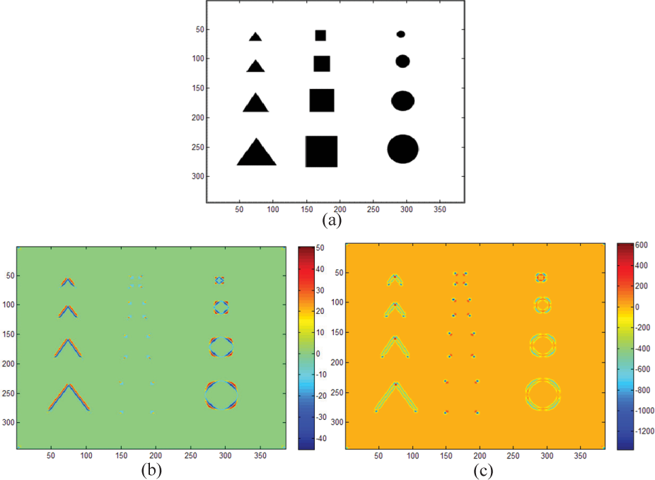
Image-based curvature estimation results: (a) Input test image; (b) implicit curvature method [3]; and (c) Gaussian curvature.

Both impHarris and impCSS corner detectors have their own advantages and limitations. In general, the impHarris corner detector is robust to textured images due to image filtering, but offers poor detection of obtuse corners and shows shifted corner positions (Figure 4). The shifted corner detection, as shown in Figure 4(a), originates from the Gaussian derivatives and the additional smoothing in the computation of the autocorrelation matrix. The impHarris detects only strong corners, such as those with an “L” shape or “T” junction, which have two significant eigenvalues. An obtuse angular structure generates only one significant eigenvalue, which leads to the corner-missing problem shown in Figure 4(b). Conversely, use of the CSS corner detector is powerful for structured objects or line drawings due to its edge-based curvature estimation, but is poor in textured images with inaccurate edge extraction (Figure 5).

Figure 4.

Limitations of the impHarris corner detector: (a) Inaccurate corner locations; and (b) missing obtuse angular corners (α = 0.06).

Figure 5.

Limitations of the impCSS corner detector: (a) Canny edge detector used in the impCSS; and (b) false corner detection due to unstable edge detection.

2.2 Proposed corner detection algorithm

As discussed previously, intensity-based corner detection is robust when used in textured images, due to its image filtering scheme, but weak when used to detect structurally meaningful corners such as obtuse angles and has low positional accuracy. In contrast, the contour-based corner detector is powerful when used to detect structured objects, due to its curvature estimation strategy, but is weak when used to detect textured images, due to its fragile Canny edge detector. The motivation of our research starts at this point: how can we use the advantages of both approaches to detect corners stably in general scenes? Since evidence exists that the human visual system pays strong spatial attention to contour curvatures [20], we use the curvature-based approach as a basic corner detector. The next question is; how to stably extract curvature information from textured or noisy images? Our approach is to adopt the underlying scheme of the intensity-based approach to alleviate the edge extraction process problem. The intensity-based method is usually based on a spatial filter. In the case of impHarris corner detector, it uses image-based filters such as the derivative filter or the autocorrelation filter. As such, we estimate the curvature information directly in the image space by eliminating the edge detection process. Figure 6 summarizes the key idea and the proposed corner detection system.

Figure 6.

Motivation of the proposed method and the related block diagram.

The proposed corner detection system consists of a spatial filtering part and a detection part. The filtering part conducts direct curvature estimation by applying the curvature filter after the orientation filter. The corner detection part performs local maxima on the curvature field and the final corners are extracted by the application of a threshold. The key aim of this paper is conducting a multi-scale curvature estimation on the intensity image space, instead of the edge-based contour space, to detect the structurally accurate corners for both textureless and textured objects. The orientation filter produces an orientation flow image, called the orientation field (OF), from an input image. Pixel-wise approximate curvature filtering on the OF generates the curvature intensity image, called the curvature field (CF). The global thresholding method detects the final corner points, after the local maxima. The spatial filter and corner detection process is repeated for the next pyramid image to detect larger structural corners. We call the proposed corner detector CF corner in the following sections. Since the CF corner detector combines the advantages of both approaches, we can expect both robust detection of structurally meaningful corners and accurate localization of the corner position, even in textured or noisy environments. This method will be validated in the experimental section.

3. Estimation of OF and CF

3.1 OF

The proposed spatial filter consists of two steps. The OF (OF(i, j)) is obtained in advance and then the CF (CF(i, j)) is estimated. Since we do not use the edge extraction process, the orientation calculation is critical to the consecutive processes. As such, an initial input of I(i, j) is pre-processed using Gaussian smoothing with σ = 1.4. The orientation of each pixel can be calculated simply using Equation (2):

O F_{s i m p l e} (i, j) = m o d {t a n^{- 1} (\frac{I_{y}}{I_{x}}), π} + \frac{π}{2}

(2)

where I_x,I_y denote the row and column directional gradient respectively, with a kernel coefficient [-1 0 1]. We use the orientation range of [0, π] instead of [-π, π] to consider shape direction only and not polarity.

A simpler orientation estimation method proposed by Kass and Witkin [6] can directly calculate orientation flow without the use of a modulus operator. They derived image flow orientation in terms of power spectrum analysis, as shown in Equation (3). This can be easily derived by vector analysis. Assume a gradient vector G = I_x + I_yi, whose power is G² = (I_x + I_yi)² = I_x² -I_y² + 2I_xI_yi. As a result, the angle of gradient power is defined as shown in Equation (3). Figure 7 shows OF examples calculated using the OF_simple and OF_flow methods. Note that both methods produce the same results. In this paper we use Equation (3) since it doesn't need the modulus computation.

O F_{f l o w} (i, j) = \frac{1}{2} t a n^{- 1} {\frac{2 I_{x} I_{y}}{I_{x}^{2} - I_{y}^{2}}} + \frac{π}{2}

(3)

Figure 7.

Orientation field estimation results: (a) OF_simplemethod; and (b) OF_flow method. The arrows indicate calculated orientations.

3.2 CF

The next step is to estimate a CF (CF(i, j)). Curvature is originally defined as the rate of change in orientation over spatial variation, as shown in Figure 8(a) [15]. Given an extracted contour, the ideal curvature is defined as Equation (4), where ΔS denotes infinitesimal contour length and δθ denotes orientation variation on the contour position.

k = \underset{Δ S \to 0}{l i m} \frac{Δ θ}{Δ S}

(4)

Figure 8.

Curvature field estimation procedures: (a) ideal curvature estimation given a contour, (b) calculated orientation field (over which the ideal contour is overlaid.), and (c) approximate curvature estimation diagram.

Since we do not use edge or contour extraction processes, we have to use an approximate curvature estimation method in the image domain. As shown in Figure 8(b), the ideal contour is quantized into pixels and the OF has implicit contour information. As such, if we carefully design a certain filter to be applied on in the OF, we can then obtain approximated curvature information. As shown in Figure 8(b), we do not have any information about contour pixels in advance, so all pixels in the OF are considered candidate contours. Curvature approximation in the OF can be achieved, as shown in Figure 8(c). Assume that the current pixel of an OF is (i, j). We can then make a local contour pixel segment using the orientation information, OF(i, j). Extending along that direction, contour segment pixels are selected in a 3 × 3 window. If we use the direction information of neighbouring pixels (OF_fwd (i, j),OF_bwd(i, j)), the approximate curvature (k_sel) can be estimated using Equation (5), where δS can be considered as 2 (pixel distance) and δθ can be approximated as the neighbouring orientation difference (θ_fwd – θ_bwd). k_sel denotes curvature estimation by neighbouring pixel selection. Neighbouring pixel pairs are selected by quantizing the direction of the centre pixel into four angles, such as 0°, 45°, 90°, 135°.

k_{s e l} (i, j) = \frac{Δ θ}{Δ S} = \frac{‖ O F_{f w d} (i, j) - O F_{b w d} (i, j) ‖}{2}

(5)

We can also consider another curvature estimation (as shown Equation (6)), in which orientation differences between neighbouring pixels and a centre pixel are calculated and summed. W denotes a local window around (i, j). In this approach we need not find the contour segments. k_sum denotes the curvature estimation by summing the orientation differences of the neighbouring pixels. A performance comparison of the curvature estimation methods will be presented in the experimental results section.

k_{s u m} (i, j) = \frac{1}{8} \sum_{(k, l) \in W, k \neq i, l \neq j} ‖ O F (k, l) - O F (i, j) ‖

(6)

However, we cannot use this curvature information because it produces many false responses around the homogeneous area, including the edges (as shown in Figure 9(b)), for a given test image (Figure 9(a)). If we use cosine angle distance [11], as shown in Equation (7), instead of the angle difference, we can enhance the curvature response while maintaining strong curvature around the homogeneous region and edges (as shown in Figure 9(c)). As such, we modify Equation (7) by adaptive weighting using gradient magnitude (M_fwd, M_bwd) as defined in Equation (8). Figure 9(d) shows the obtained CF estimation using Equation (8). Note that there are strong responses around the true corners. Some noisy curvature responses can be reduced further by a simple smoothing, as shown in Figure 9(e).

k_{c o s i n e} (i, j) = (1 - c o s (k_{s e l} (i, j)))

(7)

C F (i, j) = k_{c o s i n e} (i, j) \cdot M_{f w d} \cdot M_{b w d}

(8)

Figure 9.

Curvature estimation results using (b) k_sel, (c) k_cosine, (d) proposed, and (e) additional smoothing, for a given test image (a).

Figure 10 shows the overall corner detection procedures, using the proposed orientation and curvature filters for the OF and CF calculations. An input image consists of three regions with different shades in the rectangle. In Step 1, the modified orientation estimation filter produces the OF. In Step 2, the proposed curvature estimation filter produces the final CF. Note the curvature responses around the interior regions. We can obtain final corner detection results through a local maxima (3 × 3 window) and threshold, as shown in the block diagram of Figure 6.

Figure 10.

Example of corner detection process using the proposed direct curvature estimation method.

4. Experimental results

4.1 Evaluation criteria and standard test images

Localization accuracy: The localization accuracy can be measured using the localization error, defined as the amount of pixel deviation of a detected corner from a ground truth position [1]. It is measured as the root mean square error of the ground truth and detected corner locations, as defined in Equation (9), where N is the number of detected corners, (x_d, y_d) is the location of each detected corner and (x_t, y_t) is the ground truth location.

L_{e} = \sqrt{\frac{1}{N} \sum_{i = 1}^{N} {(x_{d} (i) - x_{t} (i))}^{2} + {(y_{d} (i) - y_{t} (i))}^{2}}

(9)

Corner detection accuracy: There are several metrics that can measure the corner detection accuracy, such as the number of true positives, the number of false positives, the detection rate and the false alarm rate. However, a corner detector critically depends upon the threshold. As a result, we use (recall vs. 1-precision) curve metrics, which can reveal the overall detector performances according to threshold variation [7, 16]. The recall value measures the number of correct corner detections out of the ground truth corners, defined as Equation (10), while the value of (1 – precision) measures the number of incorrect corners out of all possible corner detections, as Equation (11).

r e c a l l = \frac{N u m b e r o f c o r r e c t d e t e c t i o n}{N u m b e r o f t r u e c o r n e r s}

(10)

1 - p r e c i s i o n = \frac{N u m b e r o f i n c o r r e c t d e t e c t i o n}{N u m b e r o f a l l p o s s i b l e d e t e c t i o n}

(11)

Repeatability under image transformations: The above mentioned criteria, localization accuracy and detection accuracy, are defined in the still images. Another required measure is repeatability, which can measure the corner detection consistency under different varieties of image variations, such as camera position, illumination and camera motion [13, 19]. The repeatability rate for a pair of images (I₁ I₂) having (N₁, N₂) corners each and a known relative image transformation T is provided in Equation (12):

R (I_{1}, I_{2}, T) = \frac{N u m b e r o f c o r r e s n p o n d e n c e s}{m i n (N_{1}, N_{2})}

(12)

where two corner points, c₁ = [x₁,y₁]^t ∈ I₁ and c₂ = [x₂, y₂]^t ∈ I₂ are called correspond iff dist(Tc₁,c₂) < t₀, where t₀ is a pre-defined threshold.

It is important to remember that the intended application of the corner detector must be kept in mind when evaluating a corner detector. For example, in an image alignment application the localization accuracy and repeatability rate is critical, but detecting all true corners is of little importance, as long as a sufficient number of interest points are available to allow accurate alignment of the images. However, in an object recognition application, failing to detect a corner may result in a different description of the object being generated, leading to a misclassification of the object.

For the quantitative evaluations, we use the standard test images (Figure 11) that are available on the web (http://www.ee.surrey.ac.uk/CVSSP/demos/corners/originals.html). As shown in Figure 11(a), the synthetic image contains many corner types (L-Junction, Y-Junction, T-Junction, Arrow-Junction and X-Junction) and is widely used to evaluate how a corner detector responds to each of these corner types. This test image also contains corners formed at a range of different grey-scale values to test operation on corners of varying intensity. Since the majority of applications operate on real-world images, each of the corner detectors is evaluated on the three real images in Figure 11(b)–(d). The “block” image tests the operation of the corner detectors on a real image where the location of the corners is intuitively clear, the background is uniform and each object has a nearly uniform colour and texture. An image such as this is representative of the type of images required in many assembly lines or manufacturing type applications. The “house” image is a more difficult image due to the texture on the side and roof of the house and the presence of many different types of corners. This examples illustrates why a strict definition for a corner has not been established – it is unlikely different individuals would agree on exactly what parts of the image have a corner and would certainly not agree on the precise location of a given corner. The “Lab” image is also frequently used in indoor mobile robot applications.

Figure 11.

Examples of standard corner test images: (a) synthetic image, (b) block image, (c) house image, and (d) Lab image.

4.2 Parameter analysis of the proposed CF corner detector

In this section, we analyse parameters that may be used to optimize the proposed CF corner detector, in terms of multi-scale level, smoothing parameter, curvature estimate method and threshold.

Multi-scale level: The CF corner detector considers a local 3 × 3 window to estimate curvature. As a result, we need to use a multi-scale approach to detect large corner structures. In the evaluation multiple scales (1,1 / 2,1 / 4,1 / 8) are considered, but two scale levels (1,1 / 2) are enough to detect corners (Figure 12). Figure 12(a) represents the estimated CF, Figure 12(b) shows the corner candidate pixels after thresholding and Figure 12(c) shows the final detection results coming from each scale level. In this test 51 corners are detected in scale level 1 and an additional 7 corners are detected in the higher scale.

Figure 12.

Multi-scale evaluation results: (a) curvature field, (b) thresholded results, and (c) final detection after non-maxima suppression using local maxima.

Initial smoothing: We will check the initial smoothing parameter (σ), which is crucial to reduce false corner detection in noise images. We use the test image of “blocks” that has some image noise and metrics of recall vs. (1-precision) by varying the smoothing parameter σ. The ground truth corner is selected by human inspection in order to count the number of correct corners and false corners. Figure 13 shows the evaluation results by varying σ from 0.1 to 2.0. Corresponding detection examples are shown in Figure 14. According to the graph and visual inspection, σ = 1.4 is the suitable smoothing choice.

Figure 13.

Analysis results of the smoothing parameter (σ) in terms of recall vs. (1-precision) curve.

Figure 14.

Corner detection examples using (a) σ = 0.1, (b) σ = 1.4, and (c) σ = 2.0.

Curvature estimation scheme: As discussed in the previous section, there are two kinds of curvature estimation methods using k_sel or k_sum. We use the same blocks image as a test image and then check the CF estimation and final corner detection. Figure 15 shows the evaluation results. The first row represents k_sel -based approach and the second row represents k_sum -based approach. The k_sel method produces clean and strong corner responses, compared with the k_sum method (Figure 15(a),(b)). In the final corner detection, k_sum method detects 17 false corners (Figure 15(c)). As such, we use k_sel -based curvature estimation method in the following evaluations.

Figure 15.

Comparison of the curvature estimation scheme between k_sel and k_sum: (a) curvature field in scale level 1; (b) thresholded results; and (c) detected corners.

Threshold analysis: The last analysis involves inspecting the threshold values used in the final corner detection. We also use the “blocks” test image and recall vs. (1-precision) curve by varying the threshold from 0.0001 to 0.01. Figure 16 shows the evaluation results, while Figure 17 shows the detection examples. According to the graph and visual inspection, Th = 0.003 is the suitable threshold choice.

Figure 16.

Analysis results of the threshold parameter (Th) in terms of recall vs. (1-precision) curve.

Figure 17.

Corner detection examples using (a) Th = 0.0001, (b) Th = 0.003, and (c) Th = 0.01.

These evaluations are based on certain test images, in order to check nominal values, so the above parameters can be tuned depending on the test images.

4.3. Performance evaluation

Until now, we have investigated several parameters of the proposed CF corner detection. In this section the CF, impHarris and impCSS corner detectors are evaluated and compared in terms of localization accuracy, noise sensitivity, detection accuracy, repeatability to image transformation and execution time.

Comparison of localization accuracy: The first evaluation is the corner localization accuracy, which can be important to camera calibration, 3D reconstruction and so on. We use the “synthetic” test image since we know the exact corner location. The ground truth location is prepared by human vision to evaluate the location error. In addition, thresholds are tuned to produce almost the same number of corners for the CF, impHarrs and impCSS corners. Figure 18 represents the evaluation results. The squares denote the detected corners, while the crosses indicate the ground truth corner locations. The average localization error of the CF corner is 1.17 pixels, that of impHarris corner is 1.74 pixels and that of impCSS corner is 1.44 pixels. As a result, the proposed CF corner has the lowest localization error, followed by the impCSS corner and then the impHarris corner.

Figure 18.

Comparison of corner localization error using (a) proposed CF corner, (b) impHarris corner, and (c) impCSS corner, where the squares (□) represent the detected corners and the crosses (+) represent the ground truth locations.

Comparison of noise sensitivity: The second evaluation is of noise sensitivity of the corner detectors. Gaussian noise is added by changing the standard deviation from 0 to 20. In this case, we use the “blocks” image and check the recall vs. (1-precision). The threshold of each method is tuned to produce the same number of corners (around 58) at noise level 0. Figure 19 shows the comparison results. At a glance, impHarris seems to be robust to noise, the CF corner reacts normally and impCSS performs the worst. However, if we inspect the corner detection images as shown in Figure 20, impHarris generates a lot of corner detection, which leads to a high recall rate. The impCSS corner detector produces many false corners in noisy homogeneous regions. The proposed CF corner detector shows more stable detection around corners, compared with other methods.

Figure 19.

Comparison of the image noise sensitivity in terms of recall vs. (1-precision) curve.

Figure 20.

Corner detection examples at a noise level 20 using: (a) CF corner, (b) impHarris corner, and (c) impCSS corner.

Comparison of detection accuracy: The third evaluation is corner detection performance. In this case, we use a recall vs. (1-precision) curve to investigate the overall detection performance, regardless of threshold selection. The standard “blocks” image is used since the ground truth is available. The evaluation results of corner detection are shown in Figure 21. Note that the CF corner has the largest area in the recall vs. (1-precision) curve, followed by impHarris corner and finally impCSS corner. As such, we can conclude that the CF corner is the best detector.

Figure 21.

Comparison of the corner detection in terms of recall vs. (1-precision) curve.

Comparison of repeatability according to image transformation: The fourth evaluation is the consistency of corner detection in image transformations. We use a repeatability measure to quantify the consistency. Repeatability is important for detecting corners in sequences where correspondence should be achieved among image transformations. The test images include “blocks,” “house” and “lab”. The repeatability tests are conducted in terms of image rotation and scale change. As a result, we compute the repeatability by counting matched corners between a reference image and transformed images. Since the transformation value is available, we can predict the ground truth of the corner positions. Figure 22 summarizes the repeatability comparisons in terms of image rotation and scale for the standard test images. We use a rotation range of [0°,90°], with an interval of 0.5° and scale range of [1,2], with an interval of 0.1. The proposed CF corner detector shows upgraded repeatability performance compared with the impHarris and impCSS methods. Table 1 and 2 represent the average repeatability.

Figure 22.

Repeatability evaluation results for image rotation and scale using standard test images (blocks, house, lab). The row represents image type, the first column represents image rotation, and the second column represents image scale.

Table 1.

Average repeatability for image rotation.

Image	CF corner [%]	impHarris [%]	impCSS [%]
Blocks	93.5	86.2	81.7
House	82.5	67.6	78.7
Lab	95.2	97.0	86.4

Table 2.

Average repeatability for image scale.

Image	CF corner [%]	impHarris [%]	impCSS [%]
Blocks	90.8	77.5	88.2
House	91.1	74.5	88.0
Lab	95.3	95.7	86.6

Comparison of execution time: Finally, we compared the execution time. In the case of optimized code, impCSS and impHarris show 0.09sec and 0.15sec respectively. The proposed CF corner takes 0.2sec. All the programs are tested in Matlab 7.6 with i7–990x CPU for a 256 × 256 image. The C++ implementation shows 10msec for the same image.

In addition to the above quantitative evaluations, it is worthwhile to qualitatively evaluate corner detection, as shown in Figure 23. The proposed CF corner detector found the useful corners.

Figure 23.

Qualitative evaluation with related methods: (a) test image, (b) SUSAN [14], (c) CSS, (d) COP [2], (e) Harris, and (f) proposed CF

Comparison of repeatability according to viewpoint changes: Until now, we conducted the CF evaluations using four standard test images. However, it is necessary to expand the experiments for real imagery, so as to make the findings more conclusive. Since robotic applications such as mobile robot navigation and manipulation have to find corner points repeatedly according to viewpoint changes, we prepared a new test set using a turntable and a textbook. The images were acquired with an interval of 5°. The CF corner detector was compared to the impHarris and the impCSS. Figure 24 presents partial corner detection results of the proposed method, impHarris and impCSS. According to the overall evaluation results (Figure 25), the proposed CF method shows the best performance followed by the impHarris and impCSS.

Figure 24.

Repeatability evaluation examples for camera viewpoint changes: (a) proposed CF, (b) impHarris, and (c) impCSS.

Figure 25.

Repeatability evaluation results for camera viewpoint changes. The proposed CF method shows the best performance followed by the impHarris and impCSS.

Qualitative comparison using a mobile robot platform: Finally, we also applied the proposed method to a real image sequence acquired by a mobile robot (CRX-10), as shown in Figure 26. The test platform consists of a CRX-10 robot, a Sony NEX-7 camera and a HP8440P notebook. Figure 27 shows the corner detection properties of three kinds of methods in the temporal domain. The impHarris detects a number of corners around floor textures and the impCSS shows very unstable corner detection, indicated by the circle. The proposed method shows relatively stable corner detection in video sequence.

Figure 26.

Real mobile robot platform: (a) a Sony NEX-7 camera is mounted on the CRX-10 (http://cnrobot.co.kr/board.php?board=crx10) robot, (b) acquired sample image

Figure 27.

Real indoor corner extraction using: (a) CF corner, (b) impHarris corner, and (c) impCSS corner for a video sequence.

5. Conclusion

This paper proposed a new, simple, but powerful corner detection method for detecting structurally important corners using direct curvature estimation filters. Image-based corner detection such as Harris shows good detection performance to image noise, but produces incorrect corner locations or misses obtuse angular corners. The contour-based corner detection, such as the curvature scale space (CSS), can find geometrically correct positions but shows weak performance to image noise, due to a fragile edge extractor. The curvature estimation in the orientation field can complement the weak point of the CSS by introducing the filtering scheme of the Harris method. According to the parameter analyses, a multi-scale curvature field (CF) corner detector can find true corners better than the single-scale CF corner detector. The initial smoothing of a test image with σ=1.4 produces the best corner detection performance in a noisy environment. As validated by a set of experiments (localization accuracy, noise sensitivity, detection accuracy, repeatability), the use of the orientation field (OF) estimation filter, followed by the approximated curvature estimation filter, can effectively find true corners, including obtuse corners with stable corner positions and image variations, such as image rotation, scale and viewpoint changes. In general, the CF corner detector showed the best performance, followed by the Harris corner detector and the CSS corner detector. Due to the simplicity of the algorithm, the proposed corner detection method can be used in various robot vision applications, such as mobile robot navigation and manipulation. These robotic applications require real-time corner detection and accurate corner locations. In addition, the repeatability of corner points in multiframes or camera viewpoints is also critical to the robotic applications. According to the overall experiments, we can conclude that the proposed CF corner detector can be one of the suitable feature extractors in robotic applications.

Footnotes

6. Acknowledgements

This research was supported by the 2012 Yeungnam University Research Grant.

References

Awrangjeb

, 2008. Robust image corner detection based on the chord-to-point distance accumulation technique. IEEE Transactions on Multimedia 10 (6), 1059–1072.

Bae

S. C.

Kweon

I. S.

Yoo

C. D.

, 2002. COP: A new corner detector. Pattern Recognition Letters 23, 1349–13608.

Donias

Baylou

Keskes

, 1998. Curvature of oriented patterns: 2-d and 3-d estimation from differential geometry. ICIP, 236–240.

Harris

Stephens

, 1988. A combined corner and edge detector. 4th Alvey Vision Conference, 147–151.

X. C.

Yung

N. H. C.

, 2008. Corner detector based on global and local curvature properties. Optical Engineering 47 (5), 057008.

Kass

Witkin

A. P.

, 1987. Analyzing oriented patterns. Computer Vision, Graphics, and Image Processing 37 (3), 362–385.

Klippenstein

Zhang

, 2007. Quantitative evaluation of feature extractors for visual slam. Proceedings of the Fourth Canadian Conference on Computer and Robot Vision. IEEE Computer Society, Washington, DC, USA, 157–164.

Kuhnel

, 2002. Differential Geometry: Curves – Surfaces -Manifolds 2. American Mathematical Society.

Loy

Zelinsky

, 2003. Fast radial symmetry transform for detecting points of interest. PAMI 25 (8), 959–973.

10.

Mokhtarian

Suomela

, 1998. Robust image corner detection through curvature scale space. IEEE Transactions on Pattern Analysis and Machine Intelligence 20 (12), 1376–1381.

11.

Qian

Sural

Pramanik

, 2004. Similarity between euclidean and cosine angle distance for nearest neighbor queries. Proceedings of 2004 ACMSymposium on Applied Computing. ACMPress, 1232–1237.

12.

Reisfeld

Wolfson

Yeshurun

, 1995. Context-free attentional operators: The generalized symmetry transform. IJCV 14 (2), 119–130.

13.

Schmid

Mohr

Bauckhage

, 2000. Evaluation of interest point detectors. IJCV 37 (2), 151–172.

14.

Smith

S. M.

Brady

, 1997. SUSAN – a new approach to low level image processing. International Journal of Computer Vision 23 (1), 45–78.

15.

Stoker

, 1969. Differential Geometry. John Wiley & Sons Inc.

16.

Teixeira

Filho

W. C.

Gattass

, 2008. Accelerated corner-detector algorithms. BMVC. British Machine Vision Association.

17.

Tuytelaars

Mikolajczyk

, 2008. Local Invariant Feature Detectors: A Survey. Now Publishers Inc., Hanover, MA, USA.

18.

van Ginkel

van de Weijer

van Vliet

L. J.

Verbeek

P. W.

, 1999. Curvature estimation from orientation fields. SCIA, 545–551.

19.

Willis

Sui

, 2009. An algebraic model for fast corner detection. ICCV, 2296–2302.

20.

Winter

J. D.

Wagemans

, 2008. Perceptual saliency of points along the contour of everyday objects: A large-scale study. Percept Psychophys 70 (1), 50–64.

21.

Kwon

T.-B.

Song

J.-B

Kang

S.-C.

, 2010, MCL-based global localization of cleaning robot using fast rotation-invariant corner matching method. International Conference on Control, Automation and Systems (ICCAS), 1988–1992.

22.

Monasse

Morel

J. M.

, 2010, Level lines shortening yields an image curvature microscope. IEEE International Conference on Image Processing (ICIP), 4129–4132.

23.

Jeremy

M.-S.

Marco

C.-T.

Jinna

, and Pieter

, 2010, Cloth grasp point detection based on multiple-view geometric cues with application to robotic towel folding. IEEE International Conference on Robotics and Automation (ICRA), 2308–2315.