Metrological Evaluation of a Novel Medical Robot and Its Kinematic Calibration

Abstract

The vessels are twisted in a longitudinal 3D space in the lower limbs of humans. Thus, it is difficult to perform an ultrasound scanning examination in this area. In this paper, a new medical parallel robot is introduced to effectively diagnose vessel disease in the lower limbs. The robot's position repeatability and accuracy are evaluated. Furthermore, the robot's accuracy is improved through a calibration process in which the kinematic parameters are identified through a simple identification approach.

Keywords

Medical Robot Parallel Robot Kinematic Calibration Laser Tracker

1. Introduction

Ultrasound (US) scanning examination is one of the major diagnostic modalities in daily medicine. It shows advantages in low cost and non-radiation to the human body. However, a survey reveals that the repetitive strain of daily US examination over many hours causes musculoskeletal disorders to sonographers [1]. Thus, much research is engaged towards the design of medical robots to perform the US scanning examination. Furthermore, the US medical robot can collect position data during the examination process, which provides the essential information for 3D reconstruction of the scanned area.

Several works on US medical robots have been performed. A portable US medical robot was proposed in a telescanning robot project [2]. It has four degrees of freedom (DOF) and assists a doctor in controlling a US probe remotely. The robot prototype is extended to 6 DOF in the OTELO project [3]. It is agile and able to cover the large scan area. Nevertheless, the US scanning examination requires an assistant to hold the robot during the examination process. In general, the portable medical US robot does not reduce the workload of sonographers. Many US medical robot systems are developed based on industrial robots. The Hippocrate system employs a PA-10 robot arm from Mitsubishi Heavy Industry to scan the carotid artery [4]. An F3 industrial robot from CRS Robotics was used in [5] to diagnose breast cancer. A lightweight robot LWR from KUKA was used in [6] to assist the sonographer. However, the industrial robots are mostly designed for general use, and medical applications are limited due to the closed architecture of the controllers. Thus, some serial robots are designed for US medical implement, such as an abdominal US scanning robot in [7], and a self-balanced robot from the University of British Columbia [8, 9]. Serial robots, however, have relatively low stiffness and their position errors are accumulated and amplified from link to link. Besides, the motors are generally mounted on links successively. Thus, each link has to support the weight of all the subsequent links and actuators. Several medical US robots were designed with parallel structures. A parallel robot was developed to hold the US probe in [10]. It consists of three legs displaced on both sides of the patient and a probe gripper hanging over the scanned area. A cable robot was developed in the TER project [11]. A sliding mechanism was used in a parallel robot to perform echo-graphic diagnosis [12, 13]. The patient has to support the weight of the robot since the mechanism is placed on the scanning area. WTA-2R was designed to hold the US probe and perform an automated scanning based on US image feedback in [14].

The medical robots mentioned above are mainly designed for carotid or abdominal US scanning, and are not appropriate for examination in the lower limbs due to their limited workspace, dexterity, etc. MedRUE (for Medical Robot for vascular Ultrasound Examination) is a new parallel robot designed to perform US scanning examination in lower limbs, improved based on its first concept proposed in [15]. It has a longitudinal workspace aligned with the patient's leg, but relatively small size and low weight [16]. Since MedRUE needs to know the position of its end-effector with high accuracy, in order to reconstruct a 3D volume from US images it needs to be calibrated.

The calibration of a US medical robot involves probe calibration and kinematic calibration. The probe calibration identifies the constant transformation between the probe body and US image [17, 18]. However, in this article we focus only on the kinematic calibration of the robot. The kinematic calibration methods for serial robots are mostly on identifying the Denavit-Hartenberg parameters [19, 20]. These parameters are widely used to develop the kinematic model of serial robots. However, they are not always the simplest way to model parallel robots. The calibration methods of parallel robots vary depending on the different geometric structures of parallel robots. There are many calibration studies regarding planar robots, the Gough-Stewart platform and the Delta robot [21–25].

In this paper, we present a new medical robot with its repeatability and accuracy assessment. The position accuracy is improved by a calibration method based on direct position measurements with a laser tracker. The method is easy to implement on the robot without elaborate knowledge of the advanced kinematic calibration. In addition, the proposed calibration method identifies kinematic parameters individually, and the nonlinear interferences between kinematic parameters are significantly reduced. Therefore, the identified kinematic parameters are more accurate, and are important for further research, such as temporal stiffness calibration. By contrast, other calibration methods using optimization identify all kinematic parameters simultaneously [26–28]. The optimization approach may achieve better end-effector position accuracy, but it sacrifices precision for individual parameters. The MedRUE robot is briefly described in section 2 and its kinematic model and calibrated parameters are presented. Section 3 discusses the assessment of repeatability and accuracy. Then, the proposed calibration method and the result are demonstrated in section 4. At the end, a conclusion is addressed in section 5.

2. Robot description and kinematics

In this section, the new medical robot is introduced and its intuitive kinematic model is discussed. The kinematic model considers the errors of link lengths and offsets which need to be calibrated, and thereafter the calibrated parameters are listed. The robot base reference frame (Φ₀) and the world reference frame (Φ_W) are also defined in this section. The parameters to describe these two frames are identified with a laser tracker.

2.1 Introduction of MedRUE

MedRUE (Medical Robot for vascular Ultrasound Examination) is a prototype of medical parallel robot designed for the diagnosis of the peripheral arterial disease in the lower limbs.

Figure 1:

MedRUE: a new prototype of medical US robot

As shown in Figure 1, MedRUE is a 6-DOF parallel robot consisting of a robot base with a linear guide, two five-bar mechanisms and the tool part to carry the US probe. The U-shaped robot base is mounted on a linear guide (driven by actuator Q₁). The two five-bar mechanisms are assembled symmetrically on the robot's base, and are driven by actuators Q₂, Q₃, Q₄ and Q₅. Considering the first five-bar mechanism as an example, the two links driven by actuators are called proximal links, and the two links farther from the robot base are called distal links. The distal links connect at the shaft of the tool part. The tool part consists of a force/torque sensor and a dummy probe at the end. It is driven to rotate along the shaft by a small actuator Q₆ mounted on a distal link.

Since most actuators of MedRUE are located on the robot's base, the links of the five-bar mechanisms do not need to bear the heavy load of motors. Thus, the robot is relatively lightweight and agile. The linear guide extends the workspace along the length of the patient's leg and the curved distal links avoid mechanical interferences between the robot arms and the patient leg during the examination.

Frame Φ₀, also referred to as the robot frame, is defined on the robot base plate. The top surface of the robot base plate is defined as the x₀y₀ plane, and its normal is the z₀ axis. The linear guide determines the direction of the x₀ axis, and then the front side of the robot is the direction of y₀ axis. The origin of Φ₀ is located in the front centre hole of the bottom plate.

2.2 Kinematic model of MedRUE

The kinematic model of MedRUE and its kinematic parameters are illustrated in Figure 2. The two five-bar mechanisms are symmetrically assembled on the robot's base, and can therefore be modelled in the same way. As shown in Figure 2(a), the links of the i^th five-bar mechanism are named L_ij, where i = 1, 2 and j = 0, …, 4. The corresponding link lengths are denoted by l_ij. Link L_i0 is fixed on the robot's base with an angle θ_i offset. Four actuators Q_2i and Q_2i+1 are mounted on the robot's base, and the corresponding active joint variables are q_2i and q_2i+1 at A_i and C_i respectively. The other joints q_Bi, q_Di and q_DEi are passive. The two five-bar mechanisms are parallel to the y₀z₀ plane. In Figure 2(b), the tool part connects the two five-bar mechanisms at E_i (with an offset d_ei). Two universal joints are located at F_i (with an offset d_fi) to provide orientation of the probe-support. The synchronized motion (i.e., same speed and direction) of two five-bar mechanisms provide translation motions to the tool part, while the unsynchronized motion provides rotation motions. During the rotational motion, the distance variation between the two universal joints F_i is compensated by a passive translation joint located between the probe-support and F₂. Actuator Q₆ is attached on L₁₄ to provide a rotation motion of the tool part along x₀. The probe-support is considered as the wrist of MedRUE, and a reference frame Φ_w is located at its geometric centre. Axis x_w is collinear with vector $\vec{F_{1} F_{2}}$ and z_w is pointing to the probe tip.

Given the joint values (q₁ …, q_b), the forward kinematic solution of MedRUE can be obtained as follows:

Since A_i and C_i are static w.r.t. Φ₀, for the i^th (i = 1,2) five-bar mechanism, the coordinates of A_i and C_i are represented as:

a_{i} = [\begin{matrix} x_{O_{i}} & y_{O_{i}} - \frac{l_{i 0}}{2} \sin θ_{i} & z_{O_{i}} + \frac{l_{i 0}}{2} \cos θ_{i} \end{matrix}],

(1)

c_{i} = {[\begin{matrix} x_{O_{i}} & y_{O_{i}} + \frac{l_{i 0}}{2} \sin θ_{i} & z_{O_{i}} - \frac{l_{i 0}}{2} \cos θ_{i} \end{matrix}]}^{T}

(2)

where O_i is the midpoint of L_i0 with

x_{O_{i}} = d_{e i} + q_{1} + {\tilde{q}}_{1},

(3)

and ${\tilde{q}}_{k}$ is the offset error of k^th active joint. Then the coordinates of B_i and D_i are

b_{i} = a_{i} + l_{i 1} Ψ (q_{2 i} + {\tilde{q}}_{2 i}),

(4)

d_{i} = c_{i} + l_{i 3} Ψ (q_{2 i + 1} + {\tilde{q}}_{2 i + 1}),

(5)

where $Ψ (φ) = {[\begin{matrix} 0 & - \sin (φ) & \cos (φ) \end{matrix}]}^{T} .$ .

With the coordinates of B_i and D_i, all side lengths of the triangle B_iD_iE_i are known. Then, the coordinates of E_i are obtained as

e_{i} = d_{i} + \vec{D_{i} H_{i}} + \vec{H_{i} E_{i}},

(6)

where

\vec{D_{i} H_{i}} = \frac{l_{i 4}^{2} - l_{i 2}^{2} + {‖ \vec{D_{i} B_{i}} ‖}^{2}}{2 ‖ \vec{D_{i} B_{i}} ‖} u_{\vec{D_{i} B_{i}}},

(7)

\vec{H_{i} E_{i}} = \sqrt{l_{i 4}^{2} - {‖ \vec{D_{i} H_{i}} ‖}^{2}} [\begin{matrix} 0 & - 1 & 0 \\ 1 & 0 & 0 \\ 0 & 0 & 0 \end{matrix}] u_{\vec{D_{i} B_{i}}},

(8)

and u represents a unit vector. As shown in Figure 2(a), F_i has an offset d_fi−d_ei w.r.t. E_i along x₀. Thus, the coordinates of F_i are

f_{i} = D (d_{f i} - d_{e i}, 0, 0) e_{i}

(9)

where D(x,y,z) is the translation operation.

Assuming the orientation of the wrist reference frame Φ_w is represented in the XYZ Euler angles, then

R (γ, β, α) [\begin{matrix} 1 \\ 0 \\ 0 \end{matrix}] = u_{_{\vec{F_{1} F_{2}}}} = [\begin{array}{l} u_{x} \\ u_{y} \\ u_{z} \end{array}]

(10)

where R(³, β, α) is the rotation matrix. Since actuator Q₆ is fixed on L₁₄, the first Euler angle is obtained as

γ = q_{D E_{1}} + q_{6} + {\tilde{q}}_{6}

(11)

where q_{DE
₁} = atan2(−(y_{E
₁} − y_{D
₁}), z_{E
₁} − z_{D
₁}). The other two Euler angles are obtained by substituting Eq. (11) into Eq. (10):

α = \sin^{- 1} (u_{y} \cos γ + u_{z} \sin γ),

(12)

β = \sin^{- 1} (\frac{u_{y} \sin γ - u_{z} \cos γ}{\cos α}) .

(13)

Figure 2:

Kinematic model and parameters of MedRUE: (a) five-bar mechanism and robot base; (b) the tool part

Thus, the coordinates of O_w w.r.t. Φ₀ are

p_{w} = f_{1} + R (γ, β, α) {[\begin{matrix} d_{f 1} + d_{w} & 0 & 0 \end{matrix}]}^{T} .

(14)

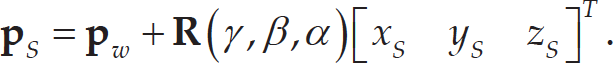
In our calibration process, a spherically mounted retrore-flector (SMR) is attached to the probe. The coordinates of the SMR centre w.r.t. Φ_w are x_S, y_S and z_S. Thus the coordinates of SMR w.r.t. Φ₀ are

p_{S} = p_{w} + R (γ, β, α) {[\begin{matrix} x_{S} & y_{S} & z_{S} \end{matrix}]}^{T} .

(15)

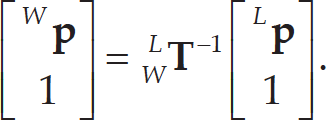
Assuming the transformation matrix from the world reference frame Φ_w to Φ₀ is represented by six parameters x_w, y_w, z_w, ³_w, β_w and α_w. Then p_S is represented w.r.t. Φ_w as:

{}^{W}p_{S} = {}_{W}^{0}T^{- 1} p_{S}

(16)

where

3. Repeatability and Accuracy Assessment

In this section, robot repeatability and accuracy are assessed before calibration. Our assessment method is an adaptation of the international standard on robot performance and test method (ISO-9283) [29]. The nominal kinematic model (i.e., the model before calibration) is assessed in this section, and the calibrated kinematic model is validated in section 4.

In the nominal kinematic model [16], the corresponding parameters of the two five-bar mechanisms in Figure 2 are identical (e.g., l_2j, = l_2j, j = 0, …, 4). Moreover, each five-bar mechanism is symmetrically designed. In other words, the proximal links are identical (l_i1 = l_i3, i = 1, 2), and so are the distal links (l_i2 = l_i4, i = 1, 2). The offset joint values are considered to be equal to zero.

3.1 Robot path design and measurement points

In our implementation, the position accuracy has the priority since it is required both for safety reasons and 3D reconstruction. Orientation errors can be compensated in the 3D reconstruction with well-developed techniques, such as scale-invariant feature transform. In this article, only the position repeatability and accuracy are studied, while the orientation is kept constant during the measurement procedure. Before taking measurements, it is necessary to define the robot trajectory and the measured positions during data acquisition.

Figure 3:

The measurement points in the workspace of MedRUE: (a) measurement points definition, (b) measurement path

Knowing that the robot is dedicated to lower limb scans, the effective robot's workspace is considered to be a half-cylinder, which covers the top surface area of a patient's leg. As shown in Figure 3(a), nine measurement points P_i (i = 1, …, 9) are considered in this target workspace. Namely, eight corners C_j (j = 1, …, 8) are created on both sides of the target workspace and form two planes C₁C₂C₇ C₈ as well as C₃C₄C₅C₆. Point P₁ is located at the barycentre of all eight corners. Point P₂ is defined on the vector $\vec{P_{1} C_{1}}$ with $‖ \vec{P_{1} P_{2}} ‖ = 0.8 ‖ \vec{P_{1} C_{1}} ‖$ , points P₃ to P₉ are similarly defined.

The used measurement path is an extension of the path design proposed in [30]. The robot end-effector is initially located at P₁ and trajectory of the robot end-effector is demonstrated in Figure 3(b). When the process started, the robot end-effector followed the trajectory on the plane C₃C₄C₅ C₆, which is composed of the sequence P₉ → P₁ → P₈ → P₁ → P₇ → P₁ → P₆ → P₁.Then, the robot trajectory continues on the plane C₁C₂C₇ C₈, and follows the sequence P₅ → P₁ → P₄ → P₁ → P₃ → P₁ → P₂ → P₁ to finish a measurement cycle. In our experiment, 30 measurement cycles are taken.

In this method, P₁ is visited from eight different directions, while all other measurement points are visited in a unidirectional approach (direction from P₁). Thus, the experiment design is used to estimate multidirectional repeatability at position P₁ and unidirectional repeatability at positions P₂ to P₈.

3.2 Accuracy and repeatability definition

At each measurement point P_i (i = 1, …, 9), the position of the end-effector is measured n times, where n = 8 directions × 30 cycles = 240 at P₁ and n = 30 at each of the other eight measurement points. A set of n measurements on a measurement point P₁ is called a cluster of P_i. For any cluster, the barycentre is defined as a virtual point whose coordinates $[\begin{matrix} {\bar{x}}_{i} & {\bar{y}}_{i} & {\bar{z}}_{i} \end{matrix}]$ are the mean values of all the n measurements:

{\bar{x}}_{i} = \frac{1}{n} \sum_{η = 1}^{n} x_{i η},

(17)

{\bar{y}}_{i} = \frac{1}{n} \sum_{η = 1}^{n} y_{i η},

(18)

{\bar{z}}_{i} = \frac{1}{n} \sum_{η = 1}^{n} z_{i η},

(19)

The distance between the η^th cycle measurement at P_i and the barycentre of the cluster of P_i is

l_{i η} = \sqrt{{(x_{i η} - {\bar{x}}_{i})}^{2} + {(y_{i η} - {\bar{y}}_{i})}^{2} + {(z_{i η} - {\bar{z}}_{i})}^{2}} .

(20)

Then the repeatability at P_i is defined as follows:

R P_{P_{i}} = {\bar{l}}_{i} + 3 S_{l i},

(21)

where and

The absolute position accuracy of P_i is defined by

A P A_{i} = \sqrt{{({\bar{x}}_{i} - {\overset{⌢}{x}}_{i})}^{2} + {({\bar{y}}_{i} - {\overset{⌢}{y}}_{i})}^{2} + {({\bar{z}}_{i} - {\overset{⌢}{z}}_{i})}^{2}},

(22)

where ${\overset{⌢}{x}}_{i}, {\overset{⌢}{y}}_{i}$ and ${\overset{⌢}{z}}_{i}$ are the command positions (reference positions) of P_i, and $\bar{x}$ , $\bar{y}$ and $\bar{z}$ are barycentre coordinates defined in Eqs. (17) to (19).

MeRUE will be used to take US images at prescribed intervals. These US images will then be used to reconstruct the 3D model of the blood vessel. For the purposes of medical examination, the accuracy in measuring the position of a given US image is important w.r.t. the neighbouring images. In other words, the relative accuracy is important for our robot.

A relative position accuracy of a point can be defined as the accuracy of the distance between adjacent points (e.g., the distance accuracy between P₁ and P₂). Since each point P_i (i = 2, …, 9) is reached starting from P_i in Figure 3(b), the nominal relative displacement of P_i (i = 2, …, 9) is calculated as follows:

{\hat{δ}}_{i} = {\hat{p}}_{i} - {\hat{p}}_{1}, i = 2, …, 9

(23)

where ${\hat{p}}_{i}$ is the nominal coordinates vector. Then Eq. (22) is modified to compute the relative position accuracy as

R P A_{i} = ‖ δ_{i} - {\hat{δ}}_{i} ‖, i = 2, …, 9

(24)

where δ_i = p_i − p_1i is the measured relative displacement based on laser tracker. The notation p_1i is the measurement value of P_i before moving towards to each P_i (i = 2, …, 9).

3.3 Experiment setup and results

The measurement setup is shown in Figure 4. The measurements are taken with a Faro Laser Tracker ION having a distance accuracy of 8 μm + 0.4 μm/m, and angular accuracy of 10 μm + 2.5 μm/m. The emitted laser is reflected by an SMR, which is magnetically attached to a nest. In our experiment, the target measurement is a 1.5 inch SMR mounted on the tool part (Fig. 4). The measured positions are expressed w.r.t. the laser reference frame (Φ_L) and transformed w.r.t. Φ_w.

We note that the measurement accuracy might be influenced by many aspects, such as environment, duration of operation, and the distance between the target and the laser tracker. Therefore, we evaluated the laser tracker accuracy for our own setup. A calibrated bar with a known length was measured ten times, and the distance error was found to be 26 μm ± 14 μm with 95.4% confidence interval of uncertainty. However, the measurement uncertainty was reduced by taking several measurements at each position.

Figure 4:

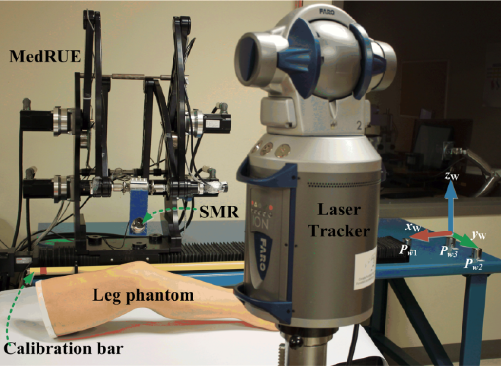
Experiment setup of MedRUE positioning performance assessment and calibration

The results for the position repeatability at the nine measurement points are shown in Table 1. The first row shows the composed repeatability defined in Eq. (21), and the other three rows list the repeatability according to the x, y and z axes. Naturally, the position repeatability at P₁ is worse, which is mainly because the arrivals at P₁ are from eight different directions. Furthermore, the position repeatability along x at P₁ is poorer than along y and z. This is caused by the fact that the motion along the x axis is dominated by the linear guide, which has a backlash of 76 μm according to its manufacturer.

Table 1.

Position repeatability (in μm)

	P₁	P₂	P₃	P₄	P₅	P₆	P₇	P₈	P₉
RP	143	141	54	60	105	99	84	77	50
RP_x	139	136	43	47	96	88	71	61	38
RP_y	74	43	39	43	48	51	52	49	39
RP_z	54	19	18	21	33	28	24	27	18

Table 2.

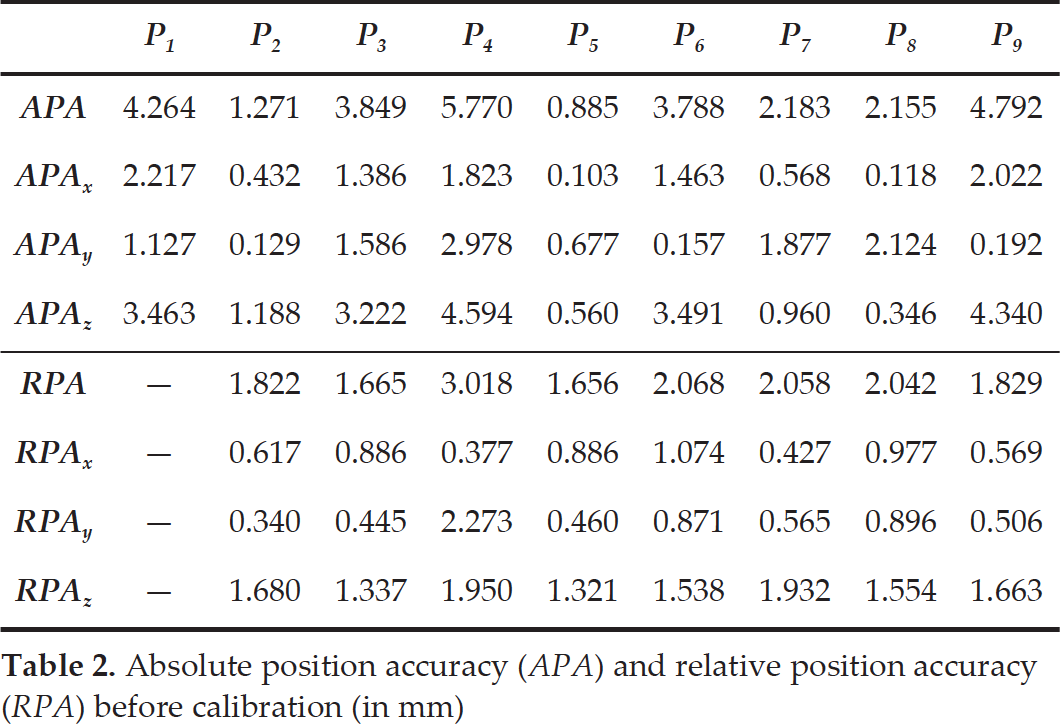
Absolute position accuracy (APA) and relative position accuracy (RPA) before calibration (in mm)

	P₁	P₂	P₃	P₄	P₅	P₆	P₇	P₈	P₉
APA	4.264	1.271	3.849	5.770	0.885	3.788	2.183	2.155	4.792
APA_x	2.217	0.432	1.386	1.823	0.103	1.463	0.568	0.118	2.022
APA_y	1.127	0.129	1.586	2.978	0.677	0.157	1.877	2.124	0.192
APA_z	3.463	1.188	3.222	4.594	0.560	3.491	0.960	0.346	4.340
RPA	—	1.822	1.665	3.018	1.656	2.068	2.058	2.042	1.829
RPA_x	—	0.617	0.886	0.377	0.886	1.074	0.427	0.977	0.569
RPA_y	—	0.340	0.445	2.273	0.460	0.871	0.565	0.896	0.506
RPA_z	—	1.680	1.337	1.950	1.321	1.538	1.932	1.554	1.663

The results for the repeatability at P₁ in the two measurement planes (i.e., planes C₁C₂C₇ C₈ and C₃C₄C₅C₆) are illustrated in Figure 5. On each plane, there are four groups (G₁ G₂, G₃, G₄) of data in different colors indicating four different directions to reach P₁ The measured data are illustrated with an asterisk marker, while the barycentre of each group is a solid circle. The cluster groups are clearly separated from each other. The divergence of measurement on P₁ shows the imperfection of the multidirectional movement caused mainly by the backlash of the mechanical parts of our robot.

The position absolute accuracy and relative accuracy before calibration is given in Table 2. As an early prototype, the robot's poor accuracy is mainly due to its manufacture and assembling errors. The worst case of the absolute accuracy before calibration is about 6 mm, while the worst relative accuracy before calibration is about 3 mm.

4. Kinematic Calibration Experiment

In this section the proposed calibration approach is explained. The actual values of the robot parameters are identified to improve robot accuracy.

Table 3.
Kinematic parameters

Group Description Parameters

(1) The world reference frame x_W, y_W, z_W, γ_W, β_W, α_W

(2) Active joint offset error ${\tilde{q}}_{2}, {\tilde{q}}_{3}, {\tilde{q}}_{4}, {\tilde{q}}_{5}$

(3) Assembling of five-bar mechanisms y_O1, z _O1 , y_O2 , z _O2 , θ₁, θ₂

(4) Link lengths of five-bar mechanisms l₁₀, l₁₁, l₁₂, l₁₃, l₁₄,
l₂₀, l₂₁, l₂₂, l₂₃, l₂₄

Group	Description	Parameters
(1)	The world reference frame	x_W, y_W, z_W, γ_W, β_W, α_W
(2)	Active joint offset error	${\tilde{q}}_{2}, {\tilde{q}}_{3}, {\tilde{q}}_{4}, {\tilde{q}}_{5}$
(3)	Assembling of five-bar mechanisms	y_O1, z _O1 , y_O2 , z _O2 , θ₁, θ₂
(4)	Link lengths of five-bar mechanisms	l₁₀, l₁₁, l₁₂, l₁₃, l₁₄, l₂₀, l₂₁, l₂₂, l₂₃, l₂₄

The parameters expected to be identified are summarized in four groups, as shown in Table 3. Parameters in Group 1 define Φ_W in Eq. (30). Group 2 represents the offset of active joints at the home position. Group 3 is named assembling parameters, which specifies how the two five-bar mechanisms are assembled on the robot base, by illustrating the position and angle of link L_i0 on the robot base (Figure 2(a)). Group 4 englobes the lengths of the links of the two five-bar mechanisms.

4.1 The world reference frame parameters

The world reference frame Φ_W is defined in the robot's workspace by three SMR nests P_W1, P_W2 and P_W3 as shown in Figure 4. Assuming P_W3 is the origin of Φ_W and P_W1 is a point on the x_W axis, then the three unit vectors of Φ_W are defined w.r.t. the Φ_L. The unit vector x_W is determined by the normalized vector $\frac{p_{W_{31}}}{‖ p_{W_{31}} ‖}$ where p_W31 is a vector from P_W3 to P_W1 in Φ_L. The z_W axis of Φ_W is defined as the normal of the plane defined by P_W1, P_W2 and P_W3. The rotation matrix of Φ_W w.r.t. Φ_L is written as:

{}_{W}^{L}R = [x_{W}, y_{W}, z_{W}] .

(25)

The transformation matrix of Φ_W w.r.t. Φ_L is defined as follows:

{}_{W}^{L}T = [\begin{matrix} {}_{W}^{L}R & o_{W} \\ 0 & 1 \end{matrix}],

(26)

where vector o_W is the composed by the coordinates of P_W3. All measured position data can be represented w.r.t. Φ_W by using the transformation matrix _W^L T. A point ^WP is derived from the laser measured data ^LP by the following equation:

[\begin{matrix} {}^{W}p \\ 1 \end{matrix}] = {}_{W}^{L}T^{- 1} [\begin{matrix} {}^{L}p \\ 1 \end{matrix}] .

(27)

For convenience, all the further measured positions, in this paper, are implicitly expressed w.r.t. Φ_W.

Frame Φ₀ is defined on the robot base plate, as shown in Figure 1. The top surface of the plate is considered as the x₀y₀ plane. By placing the SMR in n positions on the x₀y₀ plane, a reference plane is fitted from the laser tracker measurement data (3xn matrix P_n = [p₁ …, p_n], where vector p_n is the n^th measurement). The barycentre of P_n is $\bar{p} = \frac{1}{n} \sum_{k = 1}^{n} p_{k}$ . For the smallest eigenvalue of ${\bar{P}}_{n}^{T} {\bar{P}}_{n}$ (where ${\bar{P}}_{n} = [p_{1} - \bar{p}, p_{2} - \bar{p}, \dots, p_{n} - \bar{p}]$ its corresponding eigenvector approximates the normal vector z₀ of the fitted plane x₀y₀. Finally, the x₀y₀ plane is determined by a point ¯ and the normal vector z₀. The x₀ axis is aligned with the direction of the linear guide and is estimated by measuring an SMR on the robot base, while actuating the linear guide. The method to fit a line from 3D cluster points is similar to the method to estimate the normal vector z₀, except that the vector x₀ is estimated as the eigenvector with largest eigenvalue. Then, the rotation matrix of Φ₀ w.r.t. Φ_W is found as:

{}_{0}^{W}R = [x_{0}, y_{0}, z_{0}] .

(28)

The origin O₀ of Φ₀ is located on the robot base plate as shown in Figure 2(a). Its coordinates w.r.t. Φ_W are obtained by placing an SMR above the robot base plate. The projection of the SMR on x₀y₀ plane provides the coordinates of O₀ as follows:

o_{0} = {o^{'}}_{0} - (({o^{'}}_{0} - \bar{p}) \cdot z_{0}) z_{0},

(29)

where o′₀ is the vector of measured coordinates of the SMR. Then the transformation matrix of Φ₀ w.r.t. Φ_W is obtained as:

{}_{0}^{W}T (x_{W}, y_{W}, z_{W}, γ_{W}, β_{W}, α_{W}) = [\begin{matrix} {}_{0}^{W}R & o_{0} \\ 0 & 1 \end{matrix}] .

(30)

where x_W, y_W, z_W, ³_W, β_W and α_W are the Φ_W parameters to be identified: x_W, y_W, z_W are the coordinates of o₀, and Euler angles ³_W, β_W, α_W are obtained from the rotation matrix ₀^W R.

Figure 5:

Measurements at P₁ for arrivals from multiple directions: (a) on measurement plane C₃C₄C₅C₆, view in xy plane; (b) on measurement plane C₃C₄C₅C₆, view in xz plane (c) on measurement plane C₁C₂C₇C₈; view in xy plane (d) on measurement plane C₁C₂C₇C₈, view in xz plane

4.2 Active joint offset errors

The objective of this subsection is to evaluate the difference between the nominal and the real joint offsets. Active joints q₂, q₃, q₄ and q₅ are considered. As mentioned earlier, the five-bar mechanisms are symmetrically assembled, and therefore are calibrated with the same method. For simplicity, only the calibration of the second five-bar mechanism is demonstrated.

As shown in Figure 6, ten nests (N_i, i = 1, …, 10) are attached on the five-bar mechanism for measurement purpose. Four nests (N_i, i = 3, 4, 7, 10) are used in this experiment, and the remaining nests are used to identify other parameters.

Figure 6:

Experiment setup for active joint offset value estimation (nests in orange) and link length estimation (nests in orange and blue) on the second five-bar mechanism

Active joint q₄ directly drives the rotation motion of L₂₁. Thus, the joint offset error of q₄ is assessed via the evaluation of the orientation error of link L₂₁ (Figure 2(a)). The orientation of L₂₁ is determined by the coordinates of A₂ and B₂. Similarly, the joint offset error of q₅ is assessed via the orientation of link L₂₃, which is determined by the coordinates of C₂ and D₂. Two experiments are designed to obtain the coordinates of A₂, B₂, C₂ and D₂ at the robot home position. The joint offset errors are then evaluated.

Figure 7:

Path planning in the experiment of active joint offset error (i=1, 2): (a) determine coordinates of A_i and D_i, (b) determine coordinates of B_i and C_i

The first experiment is designed to determine the coordinates of A₂ and D₂ (Figure 7(a)) as follows:

Two nests denoted N₃ and N₁₀ are attached to links L₂₁ and L₂₄ respectively, as shown in Figure 6 and Figure 7(a).

The robot starts from its home position, which is illustrated with the highest transparent image in Figure 7(a). The angle of joint q₄ is increased gradually with a step of 2°, within a range of 130°. Meanwhile, link L₂₃ is kept in its home position throughout the experiment process. At each motion step the robot motion is halted, and measurements of N₃ and N₁₀ are taken.

The measured positions of N₃ and N₁₀ — which follow circular curves centred at A₂ and D₂ respectively — are fitted to two circles [31] in order to determine the coordinate of A₂ and D₂.

For illustration purposes, an intermediate position of MedRUE is illustrated with intermediate transparency, and the opaque image shows the final position of MedRUE. The nests N₃ and N₁₀ are demonstrated with a dashed circle, solid circle and filled circle in these positions, respectively.

To determine the coordinates of B₂ and C₂ we used the same approach as for A₂ and D₂. The used nests are denoted N₄ and N₇, and are attached to links L₂₂ and L₂₃ respectively, as shown in Figure 6. The experiment is illustrated in Figure 7(b).

As shown in Figure 2(a), the coordinates of A₂ and B₂ evaluate the orientation of links L₂₁ in the y₀z₀ plane. The orientation of the link L₂₁ is driven directly by active joint ˜₄. Thus, the joint offset ˜₄ is represented by the difference between the nominal value q₄ and the evaluated orientation of L₂₁ at the home position:

{\tilde{q}}_{4} = atan2 (- (y_{B_{2}} - y_{A_{2}}), (z_{B_{2}} - z_{A_{2}})) - {\hat{q}}_{4},

(31)

where y_A2 and z_A2 are the y and z coordinates of A₂ w.r.t. Φ₀. Similarly, the joint offset error of q₅ is evaluated by the coordinates of C₂ and D₂.

{\tilde{q}}_{5} = atan2 (- (y_{D_{2}} - y_{C_{2}}), (z_{D_{2}} - z_{C_{2}})) - {\hat{q}}_{5} .

(32)

The active joint offsets of q₂ and q₃, related to the first five-bar mechanism, are assessed similarly to q₄ and q₅, by using the coordinates of A₁ B₁, C₁ and D₁.

4.3 Assembling parameters

The assembling parameters are y_O1, z_O1, y_O2, z_O2, θ₁, θ₂ and these describe the assembly of the two five-bar mechanisms on the robot base. The i^th (i = 1, 2) five-bar mechanism is assembled on the robot base at joints A_i and C_i. As shown in Figure 2(a), O_i is the middle point of link L_i0 defined by A_i and C_i. Angle θ_i illustrates the orientation of link L_i0 in y₀z₀ plane. Knowing that the coordinates of A_i and C_i are obtained in the previous subsection, the assembling parameters are calculated as follows:

y_{M_{i}} = \frac{y_{A_{i}} + y_{C_{i}}}{2},

(33)

z_{M_{i}} = \frac{z_{A_{i}} + z_{C_{i}}}{2},

(34)

θ_{i} = atan2 (- (y_{C_{i}} - y_{A_{i}}), (z_{C_{i}} - z_{A_{i}})) .

(35)

Figure 8:

Experiment to assess the link length l₂₃ (a) link reference frame and nests displacement during robot motion (b) trajectory of nest N₁₀ w.r.t. to link reference frame Φ_L23

4.4 Link length parameters

The assessment of the link length parameters is demonstrated using the second five-bar mechanism (i.e., l₂₀, l₂₁ l₂₂, l₂₃ and l₂₄), while those for the first mechanism (i.e., l₁₀, l₁₁, l₁₂, l₁₃, l₁₄) are obtained similarly.

The link length of L₂₀ is determined by using the coordinates of A₂ and C₂ w.r.t. Φ₀, which were obtained in subsection 4.2:

l_{20} = \sqrt{{(x_{C_{2}} - x_{A_{2}})}^{2} + {(y_{C_{2}} - y_{A_{2}})}^{2} + {(z_{C_{2}} - z_{A_{2}})}^{2}} .

(36)

The identification of l₂₁, l₂₂, l₂₃ and l₂₄ is carried out by moving simultaneously joints q₅ and q₄ inside their limit ranges, as shown in Figure 8(a).

Note that link L₂₀ has both endpoints A₂ and C₂ fixed w.r.t. Φ₀. However, for the other links, one or both endpoints change position during the experiment. To find the position of endpoints B₂, D₂ and E₂, reference frames are attached to the corresponding links. For example, Figure 8(a) shows a link frame Φ_L23, which is associated with link L₂₃ and defined by N₅, N₆ and N₇. Therefore, the movement of the nest N₁₀, seen from Φ_L23 as shown in Figure 8(b), makes a circle centred at D₂. The coordinates of D₂ w.r.t. Φ_L23 are then transformed to be w.r.t. Φ₀.

The coordinates of B₂ and E₂ w.r.t. Φ₀ are determined in similar ways as D₂. Point B₂ is determined by observing nest N₄ in link reference frame Φ_L21 (built by nests N₁ N₂ and N₃). Then, E₂ is determined by observing nest N₄ in link reference frame Φ_L24 (built by nests N₈, N₉ and N₁₀). With all coordinates of A₂, B₂, C₂, D₂ and E₂ given w.r.t. Φ₀, the length of the links are estimated as follows:

\begin{array}{l} l_{21} = \sqrt{{(x_{B_{2}} - x_{A_{2}})}^{2} + {(y_{B_{2}} - y_{A_{2}})}^{2} + {(z_{B_{2}} - z_{A_{2}})}^{2}} \\ l_{22} = \sqrt{{(x_{E_{2}} - x_{B_{2}})}^{2} + {(y_{E_{2}} - y_{B_{2}})}^{2} + {(z_{E_{2}} - z_{B_{2}})}^{2}} \\ l_{23} = \sqrt{{(x_{D_{2}} - x_{C_{2}})}^{2} + {(y_{D_{2}} - y_{C_{2}})}^{2} + {(z_{D_{2}} - z_{C_{2}})}^{2}} \\ l_{24} = \sqrt{{(x_{E_{2}} - x_{D_{2}})}^{2} + {(y_{E_{2}} - y_{D_{2}})}^{2} + {(z_{E_{2}} - z_{D_{2}})}^{2}} \end{array}

(37)

4.5 Parameter calibration results and validation

To validate the proposed calibration method, we perform the same experiment with nominal and calibrated parameters. Both the nominal and identified values of calibrated parameters are listed in Table 4.

Table 4.
Nominal and identified parameter values

Nominal value Calibrated value

Link length of Five-bar mechanisms (unit)

l₁₀ (mm) 150 151.580

l₁₁ (mm) 400 400.510

l₁₂ (mm) 520 518.605

l₁₃ (mm) 400 400.656

l₁₄ (mm) 520 523.003

l₂₀ (mm) 150 151.007

l₂₁ (mm) 400 400.401

l₂₂ (mm) 520 523.075

l₂₃ (mm) 400 400.926

l₂₄ (mm) 520 526.285

Assembling of five-bar mechanisms (unit)

y_O1 (mm) −158 −153.714

z_O1 (mm) 308 305.442

y_O2 (mm) −158 −156.169

z_O2 (mm) 308 309.001

θ₁ (°) 150 148.906

θ₂ (°) 150 150.583

Active joint offset error (unit)

${\tilde{q}}_{2}$ (°) 0 1.445

${\tilde{q}}_{3}$ (°) 0 −0.730

${\tilde{q}}_{4}$ (°) 0 1.521

${\tilde{q}}_{5}$ (°) 0 −0.093

The world reference frame (unit)

x_W (mm) −110 −115.587

y_W(mm) −136 −140.868

z_W (mm) 30 27.452

γ_W (°) 0 0.292

β_W(°) 0 −0.057

α_W (°) 0 0.286

	Nominal value	Calibrated value
Link length of Five-bar mechanisms (unit)
l₁₀ (mm)	150	151.580
l₁₁ (mm)	400	400.510
l₁₂ (mm)	520	518.605
l₁₃ (mm)	400	400.656
l₁₄ (mm)	520	523.003
l₂₀ (mm)	150	151.007
l₂₁ (mm)	400	400.401
l₂₂ (mm)	520	523.075
l₂₃ (mm)	400	400.926
l₂₄ (mm)	520	526.285

Assembling of five-bar mechanisms (unit)

y_O1 (mm)	−158	−153.714
z_O1 (mm)	308	305.442
y_O2 (mm)	−158	−156.169
z_O2 (mm)	308	309.001
θ₁ (°)	150	148.906
θ₂ (°)	150	150.583

Active joint offset error (unit)

${\tilde{q}}_{2}$ (°)	0	1.445
${\tilde{q}}_{3}$ (°)	0	−0.730
${\tilde{q}}_{4}$ (°)	0	1.521
${\tilde{q}}_{5}$ (°)	0	−0.093

The world reference frame (unit)

x_W (mm)	−110	−115.587
y_W(mm)	−136	−140.868
z_W (mm)	30	27.452
γ_W (°)	0	0.292
β_W(°)	0	−0.057
α_W (°)	0	0.286

Figure 9:

Accuracy improvement in tracking a reference (command) line: Absolute accuracy improvement by observing the trajectory in xy plane (a) and xz plane (b); Relative accuracy improvement in xy plane(c) and xz plane (d)

MedRUE is an early prototype of a medical US robot, and there are many imperfections in its manufacture and assembling. As we can see in Table 4, there are noticeable differences between the nominal parameter values and the calibrated parameter values. The majority of errors come from the assembling of the two five-bar mechanisms on the robot base. Furthermore, the manual nest setup (as in Figure 4) for Φ_W brings noticeable errors as well. These errors are the main cause of the low accuracy before calibration, as demonstrated in Table 2.

The robot's position accuracy assessment after calibration obtained using the ISO 9283 evaluation approach is shown in Table 5. The maximum absolute position error (i.e., absolute accuracy) has been improved from 5.770 mm before calibration to 0.764 mm after calibration. The relative accuracy is also important in medical application, and its accuracy is satisfactory after calibration. The maximum relative position error was improved from 3.018 mm before calibration to 0.489 mm after calibration, as shown in Table 5.

Figure 9 illustrates the improvement of accuracy when the robot is tracking a reference command line, which is marked in a blue solid line. As shown in Figure 9(a) and Figure 9(b), which represent the trajectory projection on planes xy and xz, respectively, the trajectory before calibration has a significant error (poor absolute accuracy), and it is greatly improved after the calibration.

Figure 9(c) and Figure 9(d) illustrate the relative position offset between adjacent points. Since the reference command line is created by a set of points with constant offsets, the relative position offsets are represented as a fixed point (illustrated by an asterisk). The obtained offsets before calibration are illustrated by green squares: ideally all these squares should coincide with the reference offset (i.e., the blue asterisk mark). However, they scattered around the reference offset because of the robot parameter residuals. The obtained results (offsets) after calibration are illustrated in red triangles and it clearly demonstrates the improvement of the robot relative accuracy: i.e., the obtained relative position offsets converge towards to the reference offset.

Table 5.

Absolute position accuracy (APA) and relative position accuracy (RPA) after calibration (mm)

	P ₁	P ₂	P ₃	P ₄	P ₅	P ₆	P ₇	P ₈	P ₉
APA	0.612	0.497	0.449	0.351	0.764	0.341	0.343	0.751	0.576
APA _x	0.527	0.469	0.353	0.309	0.752	0.284	0.341	0.730	0.499
APA _y	0.235	0.152	0.228	0.158	0.053	0.122	0.040	0.165	0.284
APA _z	0.202	0.054	0.155	0.047	0.123	0.144	0.003	0.057	0.020
RPA	−-	0.259	0.382	0.253	0.276	0.489	0.396	0.294	0.201
RPA _x	–	0.066	0.132	0.156	0.157	0.313	0.249	0.254	0.029
RPA _y	–	0.107	0.029	0.058	0.212	0.103	0.235	0.070	0.076
RPA _z	–	0.227	0.357	0.191	0.082	0.361	0.198	0.130	0.184

The calibration method demonstrated in this section can be used for many other kinds of serial or parallel robots as well. As it is based on direct measurements, it provides more accurate parameter identification than conventional standard calibration methods based on optimization (e.g., forward calibration and reverse calibration method). The proposed method also requires no complex computation (e.g., identification Jacobian matrix, observability analysis) or advanced optimization knowledge in calibration. The comparison between proposed calibration method and standard calibration method are summarized in Table 6.

Table 6.

Comparison of proposed calibration method and standard calibration method

	Proposed method	Standard calibration method
Kinematic parameter identification	Individually, more accurate	All parameters identified simultaneously, less accurate
End-effector accuracy	Good	Optimized for end-effector accuracy
Complex computation	No	Yes
Robotic calibration knowledge	Basic	Advanced
Time consumption	More time for experiment	Less time for experiment, more time in method developing and computation

5. Conclusion

An assessment method of the repeatability and the accuracy of a new medical robot were presented. The complete kinematic model of the robot was introduced, and the corresponding parameters were calibrated by a direct measurement method. The proposed method is very easy to implement and requires minimum knowledge of advanced calibration techniques. This approach was validated through experiments which demonstrated a significant improvement of the position accuracy from about 6 mm before calibration to less than 1 mm after calibration. Thus, the presented method has great potential value in robot calibration when advance techniques are not available or not necessary.

Footnotes

6.

The authors thank the Canada Foundation for Innovation and the Fonds de recherche du Québec sur la nature et les technologies, who provided the funding for this project.

References

Evans

Roll

, and Baker

(2009) Work-related musculoskeletal disorders (WRMSD) among registered diagnostic medical sonographers and vascular technologists: a representative sample. Journal of Diagnostic Medical Sonography. 25(6), pp: 287–299.

Gourdon

Poignet

Poisson

Vieyres

, and Marche

(1999) A new robotic mechanism for medical application. Proc. IEEE/ASME International Conference on Advanced Intelligent Mechatronics. 2009 Sep. 19–23. Atlanta, USA. IEEE. pp: 33–38.

Delgorge

Courregès

Bassit

L. A.

Novales

Rosenberger

Smith-Guerin

Brù

Gilabert

Vannoni

Poisson

, and Vieyres

(2005) A tele-operated mobile ultrasound scanner using a light-weight robot. IEEE Transactions on Information Technology in Biomedicine. 9(1), pp: 50–58.

Pierrot

Dombre

Dégoulange

Urbain

Caron

Gariépy

, and Mégnien

J.-L.

(1999) Hippocrate: a safe robot arm for medical applications with force feedback. Medical Image Analysis. 3(3), pp: 285–300.

Nelson

T. R.

Tran

Fakourfar

, and Nebeker

(2012) Positional calibration of an ultrasound image-guided robotic breast biopsy system. Journal of Ultrasound in Medicine. 31(3), pp: 351–359.

Conti

Park

, and Khatib

(2014) Interface Design and Control Strategies for a Robot Assisted Ultrasonic Examination System. In: Khatib

Kumar

and Sukhatme

Experimental Robotics. Springer Berlin Heidelberg. pp: 97–113.

Koizumi

Warisawa

S. L

Hashizume

, and Mitsuishi

(2008) Continuous path controller for the remote ultrasound diagnostic system. IEEE/ASME Transactions on Mechatronics. 13(2), pp: 206–218.

Salcudean

S. E.

Zhu

W. FL

Abolmasesumi

Bachmann

, and Lawrence

D. P.

(1999) A robot system for medical ultrasound. Robotics research International Symposium. Snowbird. 1999 Oct. 9–12. Utah, USA. pp: 195–202.

Abolmasesumi

Salcudean

S. E.

Zhu

W. FL

Sirouspour

M. R.

, and DiMaio

S. P.

(2002). Image-guided control of a robot for medical ultrasound. IEEE Transactions on Robotics and Automation. 18(1), pp: 11–23.

10.

Onogi

Urayama

Irisawa

, and Masuda

(2013) Robotic ultrasound probe handling auxiliary by active compliance control. Advanced Robotics. 27(7), pp: 503–512.

11.

Vilchis

Troccaz

Cinquin

Masuda

, and Pellissier

, 2003). A new robot architecture for tele-echography. IEEE Transactions on Robotics and Automation, 19(5), pp: 922–926.

12.

Masuda

Kimura

Tateishi

, and Ishhara

(2001) Three dimensional motion mechanism of ultrasound probe and its application for tele-echography system. Proc. IEEE/RSJ International Conference on Intelligent Robots and Systems. 2001 Oct. 29–2001 Nov. 03. Maui, Hawaii, USA. IEEE. pp: 1112–1116.

13.

Masuda

Kimura

Tateishi

, and Ishihara

(2001) Construction of 3D Movable Echographic Diagnosis Robot and Remote Diagnosis via Fast Digital Network. Proc. 23rd Annual International Conference of the IEEE Engineering in Medicine and Biology Society. 2001 Oct. 25. Istanbul, Turkey. IEEE. pp: 3634–3637.

14.

Nakadate

Solis

Takanishi

Sugawara

Niki

, and Minagawa

(2010) Development of the Ultrasound Probe Holding Robot WTA-1RII and an Automated Scanning Algorithm based on Ultrasound Image Feedback. ROMANSY 18 Robot Design. In: Castelli

V. P.

and Schiehlen

Dynamics and Control. Springer Vienna. pp: 359–366.

15.

Lessard

Bigras

, and Bonev

I. A.

(2007) A New Medical Parallel Robot and Its Static Balancing Optimization. Journal of Medical Devices. 1(4), pp: 272–278.

16.

Zhao

Yen

A. K. W.

Coulombe

Bigras

, and Bonev

I. A.

(2013) Kinematic analyses of a new medical robot for 3D vascular ultrasound examination. Transactions of the Canadian Society for Mechanical Engineering. 38(2), pp: 227–239.

17.

Mercier

Langø

Lindseth

, and Collins

L. D.

(2005) A review of calibration techniques for freehand 3-D ultrasound systems. Ultrasound in Medicine & Biology. 31(2), pp: 143–165.

18.

Lindseth

Tangen

G. A.

Langø

, and Bang

(2003) Probe calibration for freehand 3-D ultrasound. Ultrasound in Medicine & Biology. 29(11), pp: 1607–1623.

19.

Mooring

B. W.

Driels

M. R.

, and Roth

Z. S.

(1991) Fundamentals of Manipulator Calibration. John Wiley & Sons, NY. 329.

20.

Lee

B.-J.

(2013) Geometrical Derivation of Differential Kinematics to Calibrate Model Parameters of Flexible Manipulator. International Journal of Advanced Robotic Systems. 10(106).

21.

Joubair

Slamani

, and Bonev

I. A.

(2012) Kinematic calibration of a 3-DOF planar parallel robot. Industrial Robot: An International Journal. 39(4), pp: 392–400.

22.

Joubair

, and Bonev

I. A.

(2013) Comparison of the efficiency of five observability indices for robot calibration. Mechanism and Machine Theory. 70, pp: 254–265.

23.

Zhuang

Yan

, and Masory

(1998) Calibration of stewart platforms and other parallel manipulators by minimizing inverse kinematic residuals. Journal of Robotic Systems. 15(7), pp: 395–405.

24.

Wang

Zhang

Wang

Luan

, and Tang

(2014) Accuracy Analysis of a Robot System for Closed Diaphyseal Fracture Reduction. International Journal of Advanced Robotic Systems. 11(169).

25.

Maurine

, and Dombre

(1996) A calibration procedure for the parallel robot Delta 4. IEEE International Conference on Robotics and Automation. 1996 Apr. 22–28. Minneapolis, MN. IEEE. pp: 975–980.

26.

Joubair

Zhao

L.-F.

Bigras

Bonev

I. A.

, and Loughlin

(2015) Absolute accuracy analysis and improvement of a hybrid 6-DOF medical robot. Industrial Robot: An International Journal. 42(1), pp: 44–53.

27.

Barati

Khoogar

, and Nasirian

(2011) Estimation and calibration of robot link parameters with intelligent techniques. Iranian Journal of Electrical and Electronic Engineering. 7(4), pp: 225–234.

28.

Renders

J. M.

Rossignol

Becquet

, and Hanus

(1991) Kinematic calibration and geometrical parameter identification for robots. Robotics and Automation, IEEE Transactions on. 7(6), pp: 721–732.

29.

ISO-9283. (1998) Manipulating industrial robots – Performance criteria and related test methods. International Organization for Standardization. Geneva, Switzerland.

30.

Joubair

Slamani

, and Bonev

I. A.

(2012) A novel XY-Theta precision table and a geometric procedure for its kinematic calibration. Robotics and Computer-Integrated Manufacturing. 28(1), pp: 57–65.

31.

Taubin

(1991) Estimation of planar curves, surfaces, and nonplanar space curves defined by implicit equations with applications to edge and range image segmentation. IEEE Transactions on Pattern Analysis and Machine Intelligence. 13(11), pp: 1115–1138.