
Abstract
Gene expression profiling with microarrays is a promising method to identify groups of genes, which are likely to differentiate between complex diseases, such as severe malignancies. 1,2 One problem, besides the well-known sample preparation and hybridization challenge 3 is the abundance of experimental results (typically thousands of oligonucleotide probes) for a small number of clinical samples (typically 10 to 100). Since traditional statistics require large data sets and are often tedious, I looked for a simpler and widely applicable filtering approach.
The method is based on observations obtained with artificial neural nets (ANN), which we are using for the classification of tumor genes in a similar way as described by Khan, et al. 2 An ANN in its simplest structure calculates the relationships between input patterns and their respective output classes using weight factors (Fig. 1). The higher the weight, the higher is the contribution of an input signal to the observed output pattern.
The method is based on observations obtained with artificial neural nets (ANN), which we are using for the classification of tumor genes in a similar way as described by Khan, et al. 2 An ANN in its simplest structure calculates the relationships between input patterns and their respective output classes using weight factors (Fig. 1). The higher the weight, the higher is the contribution of an input signal to the observed output pattern.
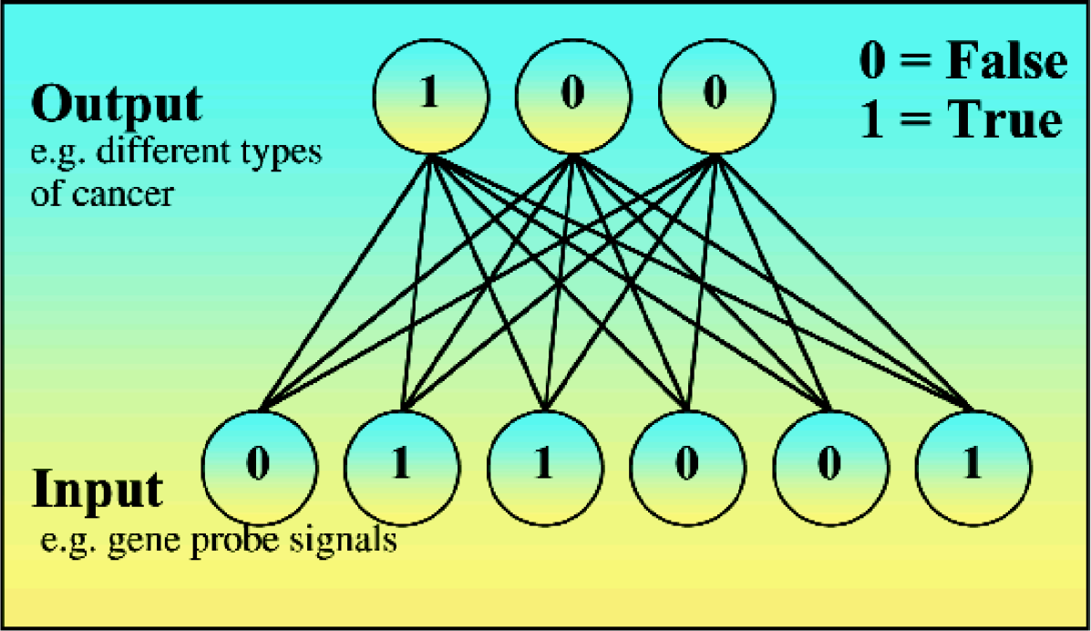
Structure of a simple neural network with six input and three output neurons, where each input neuron is connected with each output neuron. The lines in this figure represent weight factors of the artificial network after training with different patterns, e.g. 0.9 for a strong and 0,1 for a weak correlation of an input neuron signal with the observed output.
The filter mechanism described here is a simplified analogy of this traditional ANN approach:
Quantitative gene probe signals are transformed into semi-quantitative True/False results
Weights between input categories and outputs are replaced by simple “discriminators”
The algorithm describes the contribution of a distinct input (e.g. gene 1) to a defined output class (e.g. tumor A) by a single figure similar to neural net weights without undergoing the repetitive and relatively complex calculation cycles of the various ANN techniques.
Method
The filter algorithm works as follows:
Step 1: Define appropriate categories for semiquantitative results, e.g.
Step 2: Create a three dimensional array for counting results with i inputs (genes), j input categories (e.g., low, medium, high) and k outputs (e.g., tumor A and B)
Step 3: Count results falling into each of the array elements
Step 4: For each input (gene) calculate sum1 of countsj and sum2 of countsk
Step 5: Transform all counts which are different from zero into percentages of both respective sums
Step 6: Calculate discriminators for each genei as means of these two percentages
The maximum value for each gene is used for sorting. For example the results of three gene probes from five patients falling into classes A and B might be as follows:
It is obvious that gene 1 is low in A and gene 2 is high in B, whereas the rest is normal with some “noise”. Applying the filter, genes 1 and 2 receive a 100% discriminator in their respective categories low and high, whereas the rest should be below 100%.
Results
The 3-dimensional array and the calculation procedure for table 1 are illustrated in fig. 2. A discriminator of 100% can only be achieved if a positive count is surrounded by zero counts in the respective row and column. If there are further counts in any of the neighbour classes or categories (i.e., columns or rows), the discriminator will be reduced due to the degree of “noise”. As expected, the “low” category of gene 1 receives a 100% discriminator for tumor A and so does the “high” category of gene 2 for tumor B. Gene 3 receives a maximum of 83% for “normal”, due to the fact that this gene is normal in tumor A and a mixed type in tumor B.
Example set of raw data.

We tested this algorithm with simulated and real gene chip data using Excel™ spreadsheets and Visual Basic for Applications™ to implement the algorithm plus a few helpful features such as color coding and sorting. Figure 3 shows a sample of original data from an experiment with over 5,000 gene probes, tested in five controls and seven patients with two types of leucemia. Applying our algorithm to this set of data resulted in a well-ordered list of probes (Figure 4), where those probes discriminating best were ranked on top. The patterns are easy to interpret in terms of over- and under-expression of the various genes.
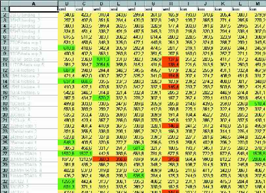
Part of an unsorted list of original data. More than 5,000 genes (column A) were tested in controls as well as in patients with two different malignancies (details are beyond the scope of this paper). Underexpressed genes are marked in red, overexpressed genes in green. A typical scatter of low (red), high (green) and normal (yellow) values can be seen.
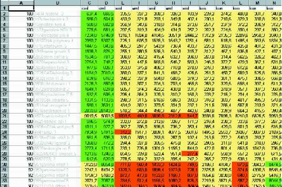
Sorted list of data after transformation with the filter algorithm. Maximal discriminators of 100% and 92% are shown in column A. Cases are sorted by class (two columns for disease A and 5 columns for disease B, followed by normal controls). There is a strong evidence that class A might be characterized by overexpression and B by underexpression of a small number out of the 5,000 genes on the test chip.
On a standard office PC, this filtering experiment with more than 60,000 individual results took about four minutes. Subsequent analysis of the 58 best-performing probes (about 1%) with a neural net took less than one minute and resulted in 100% reclassification after three training cycles. In contrast, applying the full set of data to neural net analysis required more than one hour per training cycle and still had several mismatches after three cycles. These figures must not be taken absolutely, because the performance of a net depends on many variables including the PC processor and the neural network algorithm, but the relative times clearly illustrate the usefulness of the filter.
Discussion
Several algorithms such as clustering 1 and artificial neural networks 2 have been applied to gene expression data for similar purposes. Most of them require specific computer programs or software development skills for implementation, and some depend on Gaussian distribution and large data sets for valid results.

The discriminator algorithm described here is simple and fast and can be implemented on any spreadsheet such as MS Excel™. Since the filtered patterns are easy to read (see Figure 4), even a novice in mathematics can pick the most promising genes from a color-coded table and test them with more sophisticated methods. The filter has been developed quite empirically for the fast and efficient pre-selection of gene probes and is meant as a supplementary tool for statistical pattern recognition methods. The author would like to offer help to scientists, who want real-world data to be tested with both the neural net and the simplified filter approach presented here, as long as they can be converted into the format shown in Table 1.
Acknowledgement
The author wishes to thank Holger Mueller, M.D., head pathologist at Klinikum am Eichert, Goeppingen, Germany for fruitful discussion and critique.