Fluid Thermodynamic Simulation of Ti-6Al-4V Alloy in Laser Wire Deposition

Abstract

A 3D numerical model of heat transfer and fluid flow of molten pool in the process of laser wire deposition was presented by computational fluid dynamics technique. The simulation results of the deposition morphology were also compared with the experimental results under the condition of liquid bridge transfer mode. Moreover, they showed a good agreement. Considering the effect of recoil pressure, the morphology of the deposit metal obtained by the simulation was similar to the experiment result. Molten metal at the wire tip was peeled off and flowed into the molten pool, and then spread to both sides of the deposition layer under the recoil pressure. In addition, the results of simulation and high-speed charge-coupled device presented that a wedge transition zone, with a length of ∼6 mm, was formed behind the keyhole in the liquid bridge transfer process, where the height of deposited metal decreased gradually. After solidification, metal in the transition zone retained the original melt morphology, resulting in a decrease in the height of the tail of the deposition layer.

Introduction

Ti-6Al-4V alloy is the most widely studied titanium alloy in the field of additive manufacturing (AM), which is suitable for a variety of AM techniques, such as Selective Laser Melting (SLM), electron beam selective melting (EBM), arc wire additive manufacturing (WAAM), laser wire deposition (LWD), and so on. Many computational fluid dynamics (CFD) models for different AM techniques were developed to study the morphology of molten pool and the final solidification structure of Ti-6Al-4V alloy during AM process. Guss and colleagues¹ simulated the molten pool flow in the process of SLM and explained the ablation phenomenon caused by laser.

Ge et al.² explained the formation mechanism of balling defect and distortion pattern in the process of EBM by CFD model, which has showed good agreement with the experimental results. Bai et al.³ presented a 3D CFD model to study the fluid flow and heat transfer behavior during the multilayer deposition of WAAM. And it showed that the Marangoni force was the key factor affecting the fluid flow in each layer deposition. However, there is no report on the CFD simulation of LWD of Ti-6Al-4V alloy at present.

LWD is a very complex multiphysical phenomenon coupling process, which involves the interaction above metal surface (including wire and substrate) and laser-induced metal nanoparticles on the reflection, scattering, and absorption with laser. In addition, it also involves the flow of the molten pool and the transition behavior of the molten metal. Researchers have made a lot of efforts to reveal the coupling of multiphysical phenomena in the process of LWD. For example, Torkamany et al.⁴ observed the metal transfer behavior through high-speed charge-coupled device (HCCD).

He presented that the recoil pressure was the main driving force that drove the molten metal to flow downward from the tip of the wire. Yu et al.⁵ revealed that the transition behavior of molten metal in the process of LWD can be divided into three different forms: explosive, big droplet, and molten metal bridge. Ma et al.⁶ and Abioye et al.⁷ believe that the deposition process was the most stable when the molten metal was in the transition of metal bridge.

There are few reports on the numerical simulation of LWD. Wei et al.⁸ established a multiphase model to investigate the free surface flow and temperature field evolution in the process of laser hot wire deposition. Moreover, Gu and Li⁹ have proposed a CFD transient model under the condition of extreme gravity and pressure during the process of LWD in space. The simulation results indicated that the surface tension would dominate the dynamics of the molten pool when the gravity decreases, thus resulting in irregular deposition tracks. In all the above studies, the wire feeding process was simplified and the interaction between wire and laser was ignored.

Furthermore, their heat source was added by a simple body heat source. As a consequence, it was impossible to accurately predict the transition dynamic behavior of molten metal. To reveal the dynamic mechanism of the transition behavior of molten metal during LWD, Hu et al.¹⁰ developed a 3D CFD model to investigate the fluid dynamics during liquid bridge transfer in the process of 304L stainless steel LWD. Simultaneously, they proposed that the stable progress of liquid bridge transfer can be ensured when the slenderness index (Sl) was ∼3.17–4.57. In his simulation model, the shielding effect of laser-induced metal nanoparticles was ignored, although they used the beam tracing method to simulate the reflection and absorption of laser.

Chatterjee and Chakraborty¹¹ proposed laser-induced metal nanoparticles have a strong shielding effect on laser, which reduces the absorption of laser energy by the workpiece. In this study, the shielding effect of metal nanoparticles was considered. Besides, the fluid dynamics behavior of molten metal liquid bridge transfer in the process of LWDed Ti-6Al-4V alloy was investigated. Finally, the dynamic behavior of the molten metal was predicted and the temperature history of the molten pool boundary was extracted from the model to better understand the effect of temperature on grain growth.

Experimental and Simulation

Experiment

The fluid dynamics behavior of liquid bridge transfer in the process of LWDed Ti-6Al-4V was studied by means of experiment and simulation. In addition, the LWD experimental platform used in this study was composed of 4 KW fiber laser (IPG-YLS-4000 fiber laser), Yaskawa robot, high-purity argon protective cover, and automatic wire feeder. In addition, HCCD was set up to observe the transition behavior of liquid metal at the front of molten pool during single-pass deposition, as shown in Figure 1. The Ti-6Al-4V wire (grade 5) with a diameter of 1.2 mm was selected as the filling material and the Ti-6Al-4V rolled plate (grade 5) with thickness of 10 mm as the substrate. The inclination angle of the wire was 45°. And the deposition parameters are shown in Table 1.

FIG. 1.

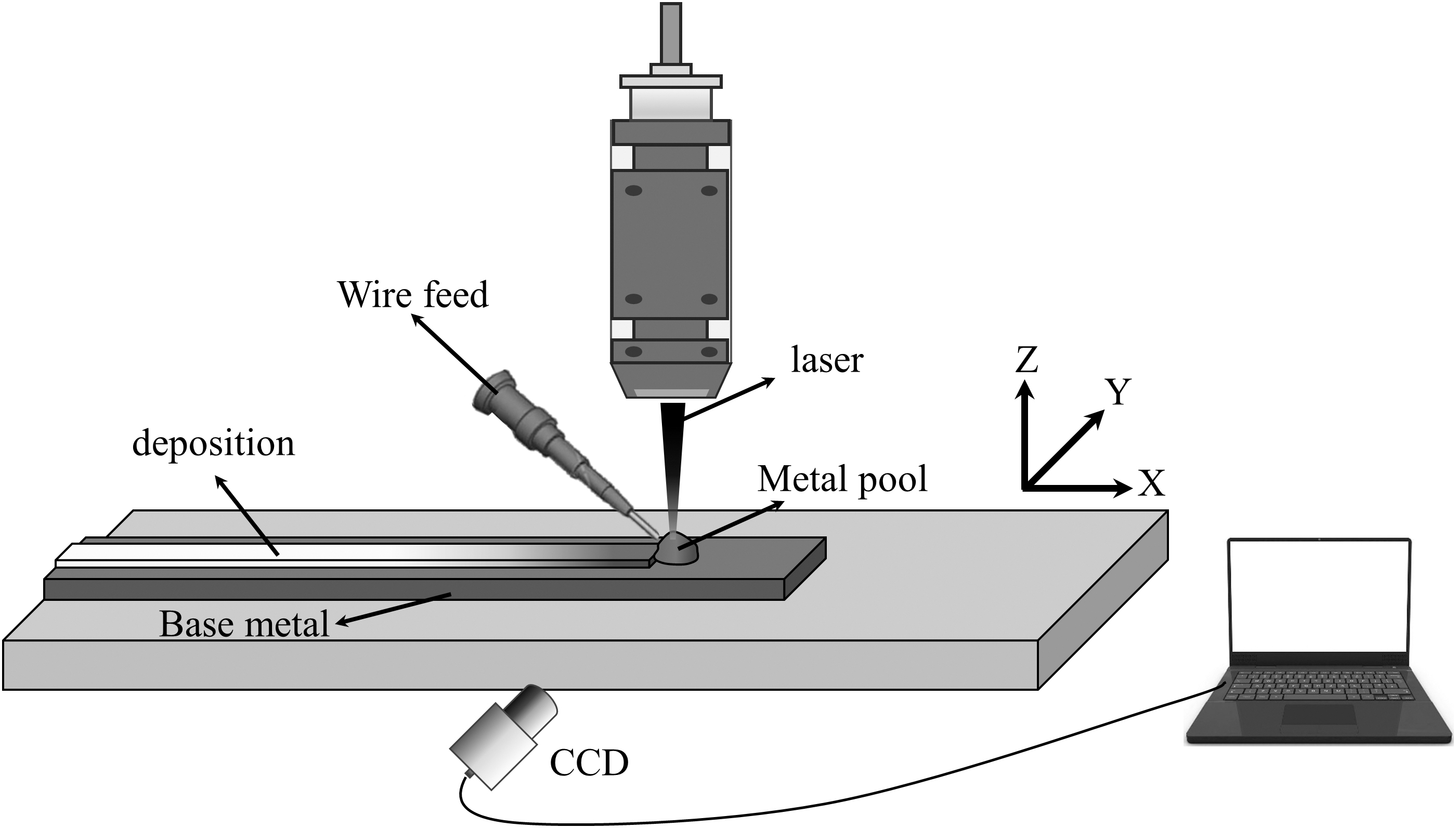
Illustration of laser wire deposition process.

Table 1.

Process Parameters

Power, KW	Wire feed, m/s	Deposition speed, m/s	Focal offset distance, mm
3000	0.064	0.026	10

The metallographic specimens were taken on the cross-section of the deposition layer after the deposition experiment. Afterward, the abrasive paper with a roughness of 80 mesh was used to polish it. Then the roughness was gradually reduced until it was polished with 5000 mesh abrasive paper. Finally, the specimens were elaborately polished by applying silica suspension. Before the metallographic photograph was taken, the sample was corroded for 5 s with Kroll's reagent (10 mL of HF, 30 mL of HNO₃, and 130 mL of H₂O).

Simulation

Governing equation

Assuming that the fluid is an incompressible fluid, the mass conservation equation of three-dimensional flow can be obtained from Wu et al.¹² $\nabla \cdot v = \frac{{\dot{m}}_{s}}{ρ}$ (1)

where $ν$ is the flow velocity of liquid metal fluid, ${\dot{m}}_{s}$ is the rate of volume mass source, and $ρ$ is metal density. Using the volume of fluid technology, the mass conservation can be re-expressed by scalar F, which is the volume fraction of fluid in the grid element defined in numerical simulation. As a consequence, the volume fraction and volume mass source rate of the fluid can be defined as Equations (2) and (3), respectively: $ρ_{0} = ρ \cdot F$ (2) ${\dot{m}}_{s} = ρ \cdot \dot{F}$ (3)

where $ρ_{0}$ refers to the density of the metal fluid in the element (the ratio of the mass of the fluid in the element to the volume of the element) and $ρ$ is the density of the metal fluid; F is the volume fraction of the fluid in element. The equation of mass conservation related to F is derived from Equations (1), (2), and (3) to Equation (4): $\frac{\partial F}{\partial t} + \nabla \cdot (ν F) = \dot{F}$ (4)

Assuming the fluid is laminar, the momentum conservation equation is as follows: $\frac{\partial v}{\partial t} + ν \cdot \nabla_{ν} = - \frac{1}{ρ} \nabla P + μ \nabla_{ν}^{2} + \frac{{\dot{m}}_{s, w}}{ρ} + G$ (5)

where P is the hydrodynamic pressure, $μ$ is the viscosity, and G is the body acceleration due to body force. In addition, ${\dot{m}}_{s, w}$ is the source term corresponding to the momentum addition rate of the filled wire.

The heat input from the laser beam is applied as the surface heat flux boundary condition in the simulation. The heat is convective and transmitted through the molten pool and the substrate, and the energy conservation equation is as follows:

where h is the enthalpy, k is the thermal conductivity, and ${\dot{h}}_{s}$ is the source term of the enthalpy rate of the filled wire.

Boundary conditions and physical parameters

Simulation was performed on Flow-3D, and the boundary conditions and the three-dimensional model are presented in Figure 2. All the boundary conditions are pressure boundary conditions. The moving flux of laser energy and wire mass sources is incorporated into the calculation domain above the top surface of the substrate to simulate the input of mass, energy, and momentum of laser heating and filling wire. The diameter of the wire is 1.2 mm and the thickness of the substrate is 6 mm. The initial temperature of the wire and the substrate is equal to ambient temperature. The mesh of the wire deposition region is refined by the transition mesh method and the mesh size of the refined area is 0.075 mm, as shown in Figure 3.

FIG. 2.

Models of substrate and wire and their boundary conditions.

FIG. 3.

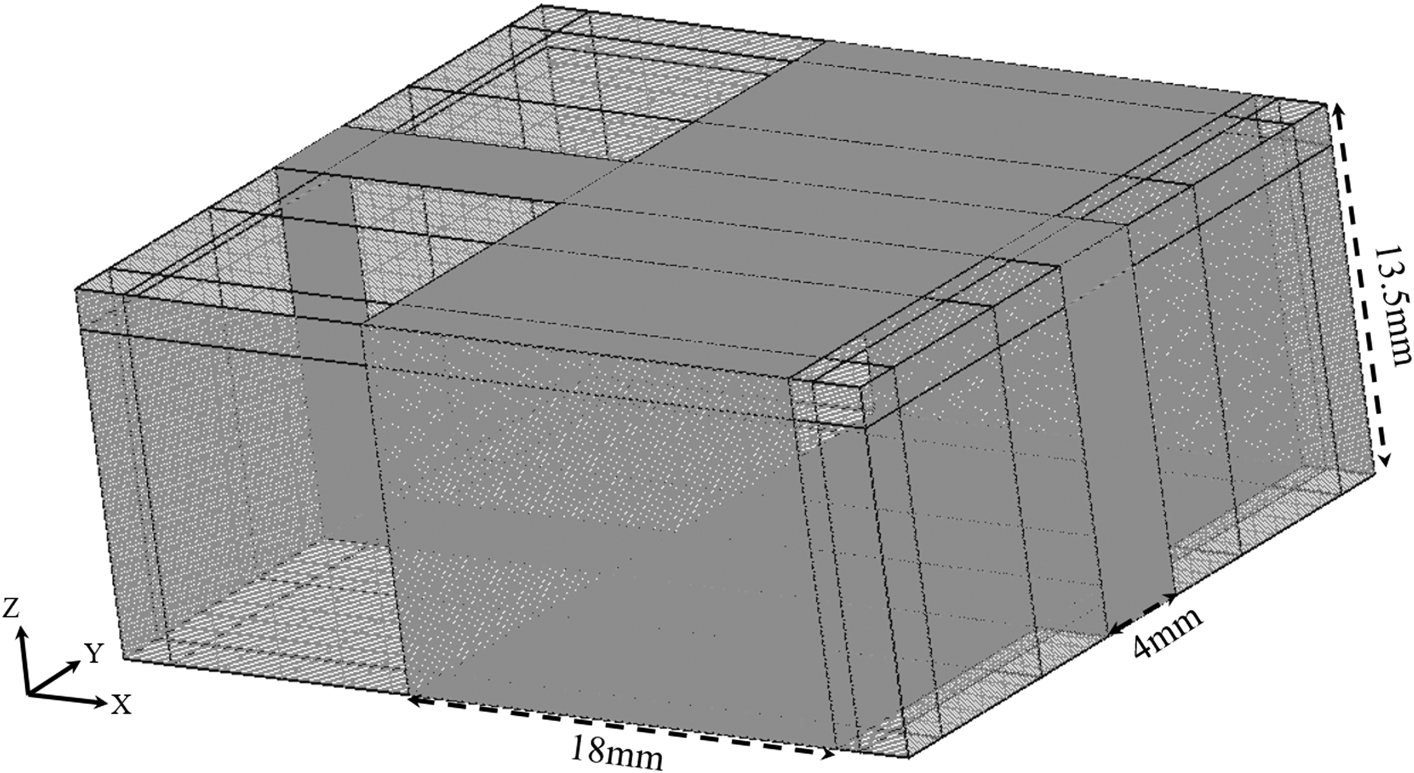
Schematic diagram of the refinement mesh.

It is assumed that the ambient temperature of the material and the surrounding environment is 297K. In addition, the material filling wire and substrate is Ti-6Al-4V alloy and its physical parameters used in this simulation are presented in Table 2.

Table 2.

Physical Parameters of Ti-6Al-4V Alloy^13–16

Property	Value
Density, $ρ_{S}$ , kg/m³	4430
Thermal conductivity of solid metal, k_S, W/m/K	32.5
Thermal conductivity of liquid metal, k_L, W/m/K	20
Specific heat of solid metal, C, J/kg/K	763 T ≤ 1923K
Specific heat of liquid metal, C, J/kg/K	872
Dynamic viscosity, $μ$ , kg/m/s	0.00325
Latent heat of melting, h, J/kg	2.86 × 10⁵
Surface tension, σ, N/m	1.68
Surface tension gradient, A, N/m/K	−2.6 × 10⁻⁴
Melting point, T_m, k	1933

Physical model

Heat source model

The laser heat source model used in this study was obtained from Cho and Na¹⁷:

where P is the laser power and $r_{0}^{2}$ is the laser spot radius. (1) Laser beam is defined as a bundle of rays, and all the rays are composed of subrays. In other words, one ray could be divided into multiple subrays, and all sub-rays have the same starting point. (2) The subrays move step by step, and at the end of each analysis step, judge whether the subray is in contact with the free surface. (3) If the located cell is not the surface cell, repeat step 2, and when the location of the ray is the surface cell, contact checking is performed. (4) If the one ray makes contact with the surface cell, various events occur, such as absorption, reflection, transmission, and scattering.

If the number of subrays in one ray is N, the number of reflected subrays is almost “RN” and the number of nonreflected subrays is almost “(1 − R)N.” R is the reflectivity of the material, which is obtained from the Fresnel-reflection model. (5) Nonreflected subrays will be absorbed at the reflection point or transmitted into the workpiece. If absorption occurs, all the energy of one subray is absorbed and ray tracing is over. In other events, such as reflection, transmission, and scattering, the direction of one subray is changed. If one subray is located outside the simulation domain, ray tracing is over. (6) Repeat steps 4 and 5 for all subrays in one ray. More details of the ray tracking process can be found in a previous study.¹⁸

Recoil pressure model

The greatest driving force of keyhole formation is the pressure caused by metal evaporation during the process of LWD, which is called recoil pressure. The recoil pressure model used in this study was adopted from Allmen¹⁹:

where P_sat is saturated pressure, P₀ is atmospheric pressure, Lv is latent heat of evaporation, and T_b is boiling point temperature. In addition, R is general gas constant.

Marangoni flow model

The surface tension acts on the surface of the molten metal-induced surface fluid flow from low to high surface tension regions, which is called Marangoni flow. The values of surface tension used in the simulation were calculated by Equation (9):

where $σ_{0}$ is the surface tension of the metal at melting point, and A is the surface tension gradient. In addition, T_m is the melting point of the metal.

Laser absorption model of laser-induced metal nanoparticles

The metal nanoparticles will not only scatter but also absorb the laser energy when the laser contacts with the metal nanoparticles in the plume region, which reduces the energy of the laser. The Beer-Lambert method is used to calculate the laser absorption probability of nanoparticles. And the absorption probability A was obtained from Dobson²⁰:

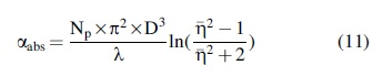
where l is the laser propagation length, N_p is the number density of metal nanoparticles, and D is the diameter of metal nanoparticles. In addition, $\bar{η}$ is the complex refractive index.

Laser scattering model of laser-induced metal nanoparticles

Generally speaking, scattering means that light or waves pass through an inhomogeneous medium. They are forced to deviate from the original direction of motion before they come into contact because of the strong repulsive force between the two sides when the two sides are close to each other. In the process of LWD, the fine metal particles scatter the laser when the laser beam passes through the plume region.

To simulate this phenomenon, we add the scattering model to the numerical model. Researchers^21–23 pointed out that the size of metal nanoparticles in the plume region was ∼100 nm, which was smaller than the wavelength of the fiber laser mainly used in this study. As a consequence, it follows the Rayleigh scattering model. Beer-Lambert scattering law is used to calculate the probability of scattering “S,” as proposed by Barber²⁴: $α_{s c a} = \frac{2 \times N_{p} \times π^{5} \times D^{6}}{3 \times λ^{4}} (\frac{{\bar{η}}^{2} - 1}{{\bar{η}}^{2} + 2})$ (13)

As shown in Equations (11) and (13), the number density of metal nanoparticles is the key role for calculating the laser absorption coefficient and scattering coefficient. N_p can be expressed as an Equation (14) according to the law of conservation of mass. $N_{p} = \frac{m}{4 ∕ 3 \times π \times {(D ∕ 2)}^{2} \times ρ \times V}$ (14)

where m is the mass of vaporized metal. In addition, V is the volume of metal after vaporization. Assuming that the volume of vaporized metal is the same as the volume of metal vapor ejected from the keyhole, V can be expressed as Equation (15) according to the ideal gas formula: $V = \frac{n R T}{p}$ (15)

where n is the molar amount of vaporized metal, which is expressed by Equation (16), R is the ideal gas constant (8.314), P is ambient pressure (10,124 Pa), and T is ambient pressure. $n = \frac{m}{m m o l}$ (16)

where, m_mol is the molar mass of the metal. Simultaneous expressions (14), (15), and (16) are as follows: $N_{p} = \frac{6 p m^{m o l}}{π D^{3} R T ρ}$ (17)

Supposing m_mol is the molar mass of titanium (47.87), T is set to 6000 K, the calculated Np is ∼4.3 × 10¹⁶, and α_abs is ∼42.

Results

Figure 4 presents the HCCD image of Ti-6Al-4V alloy in the process of LWD. It can be seen that under the experimental conditions, the molten metal was deposited in the form of liquid bridge transfer from the results of HCCD. As shown in Figure 4a, plasma plume was generated on the tip of wire under the laser irradiation. In addition, a keyhole was generated at the front of the molten pool. The molten metal flowed into the molten pool continuously from the tip of the wire by liquid bridge. In addition, it converged to form a complete deposition layer through the flow of the molten pool. As presented in Figure 4f, there was a wedge transition zone, with a length of ∼6 mm behind the molten pool.

FIG. 4.

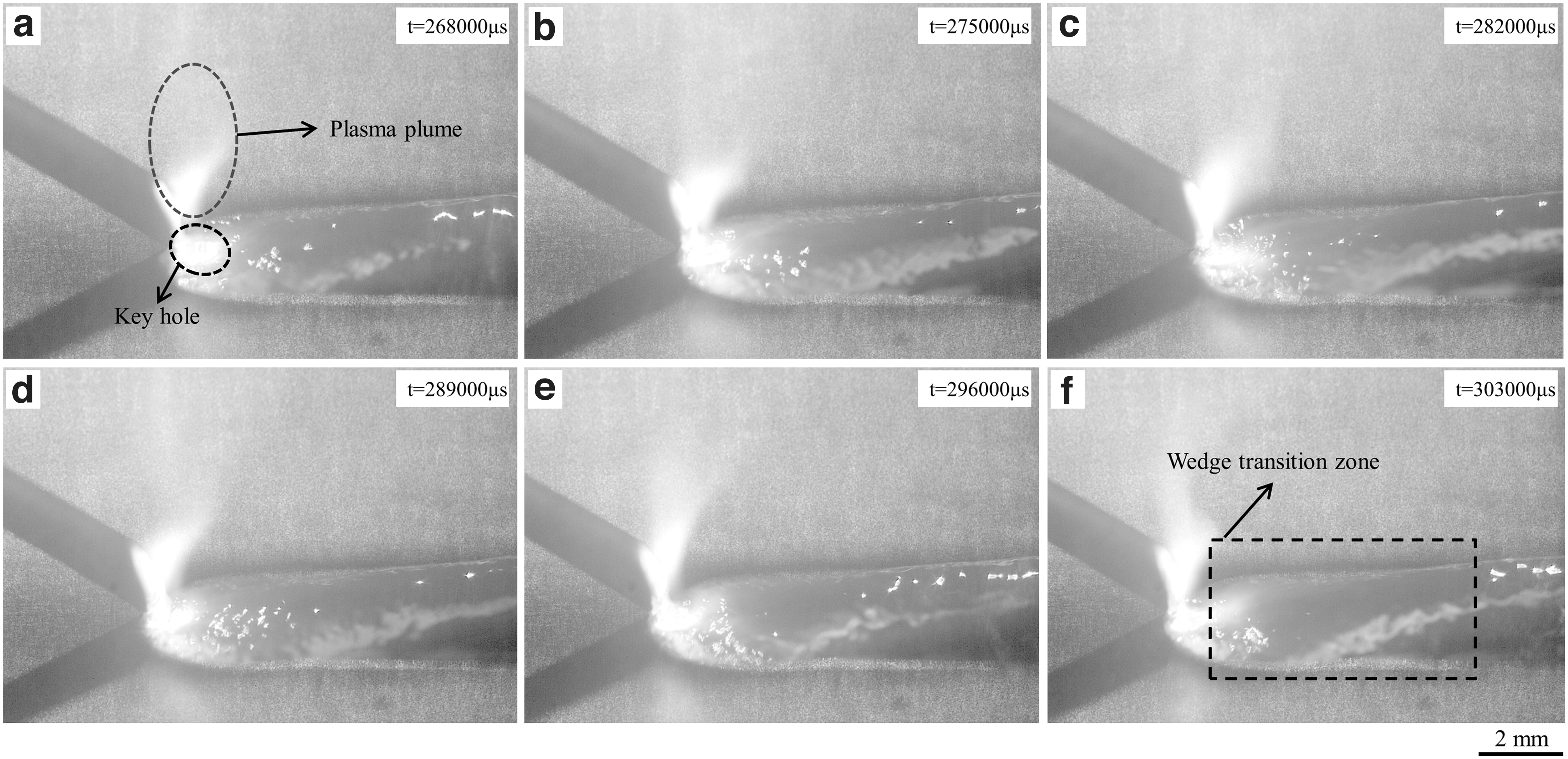
HCCD photography at different times in the process of laser wire deposition of Ti-6Al-4V alloy. (a) t = 268,000 μs; (b) t = 275,000 μs; (c) t = 282,000 μs; (d) t = 289,000 μs; (e) t = 296,000 μs; (f) t = 303,000 μs. HCCD, high-speed charge-coupled device.

In this transition zone, the height of the molten metal increased with the increase of the distance from the keyhole. The height of the molten metal tended to be stable after leaving the transition zone. From this, it could be inferred that there may be a violent flow in the molten pool.

Numerical simulation under the same process parameters was carried out to reveal the physical behavior of molten pool in liquid bridge transfer mode. Figure 5a to d show the evolution process of macroscopic morphology of deposited layer at different time during CFD simulation of LWD. As can be seen from Figure 5a to d, the molten metal entered the molten pool and spread behind the molten pool, followed by the formation of a deposition layer during the deposition process. When the deposition time was between 0 and 0.2 s, the height of the molten metal deposition layer increased gradually.

FIG. 5.

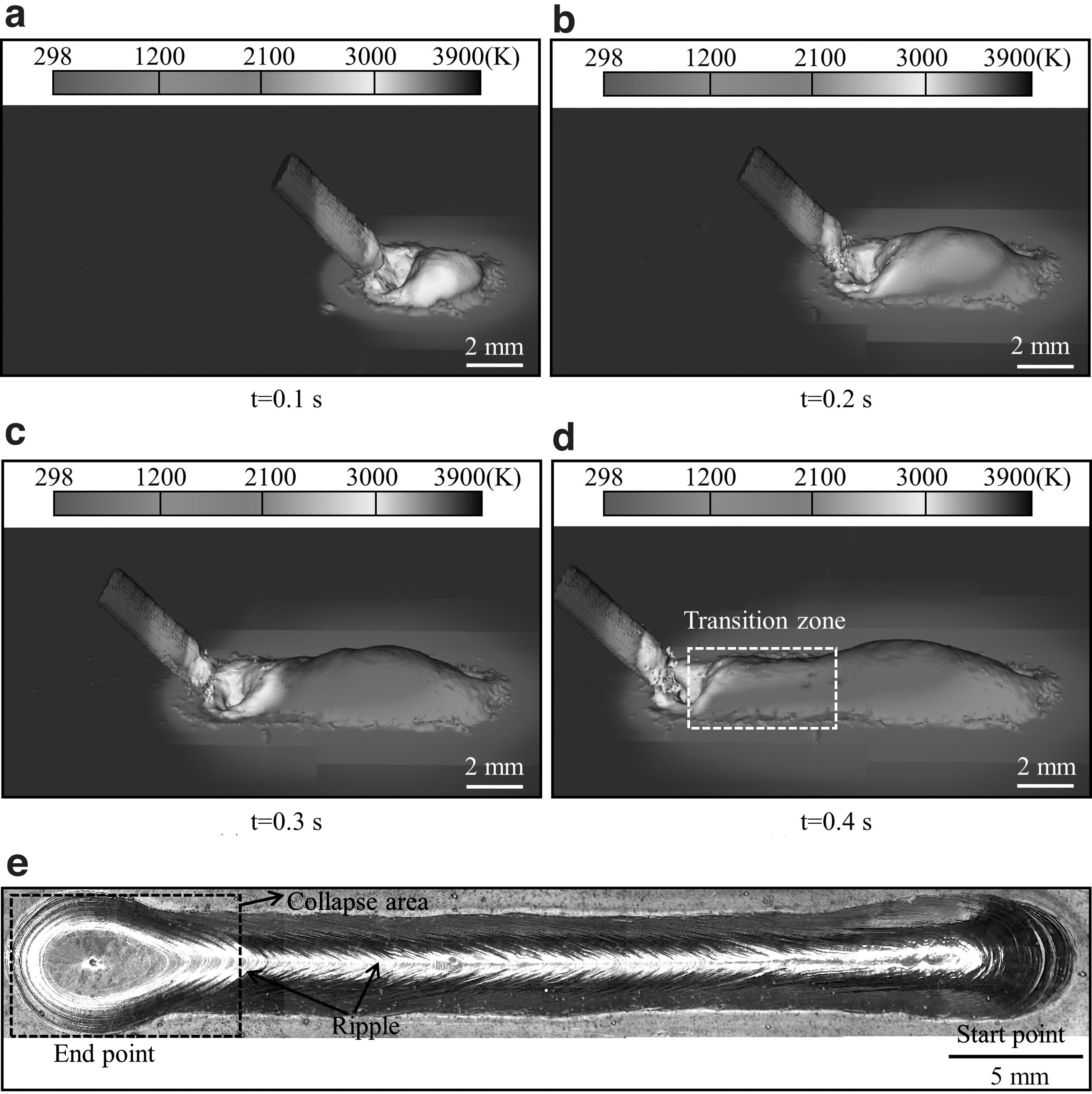
CFD simulated the evolution of the macroscopic morphology of the deposited layer at different times in the process of laser wire deposition of Ti-6Al-4V alloy and the experimental results of the macroscopic morphology of the deposited layer. (a) t = 0.1 s; (b) t = 0.2 s; (c) t = 0.3 s; (d) t = 0.4 s; (e) the experimental results of the macroscopic morphology of the deposition layer. CFD, computational fluid dynamics.

In addition, when the deposition time was between 0.2 and 0.4 s, a transition zone was gradually formed behind the molten pool, which was similar to the experimental results. The height of the deposited metal in the transition zone was lower than that outside the transition zone. Figure 5e shows the macroscopic morphology of the deposited layer produced by LWD of Ti-6Al-4V alloy under experimental conditions. The surface of the deposited layer was very bright, but many wavy stripes distributed on the surface, which were symmetrically distributed along the center line of the deposited layer. At the tail of the deposition layer, a collapse area with a gradually decreasing height was formed.

Figure 6a and b compare the experimental and simulation results of the cross-section of the deposition layer. There is a quantitative comparison of melt width, depth, and height in the figure. The cross-section in the simulation result was located in the stable zone behind the transition zone. In addition, the cross-section in the experiment sample was in the middle of the deposition layer. The width, depth, and height of the melt obtained from the experiment were 3.5, 1.6, and 1.2 mm, respectively. The simulated width, depth, and height of the melt were ∼3.3, 1.6, and 1.3 mm, respectively. It could be found that the predicted results were close to the experimental. The comparisons prove that the proposed model could accurately predict the transition behavior of molten metal.

FIG. 6.

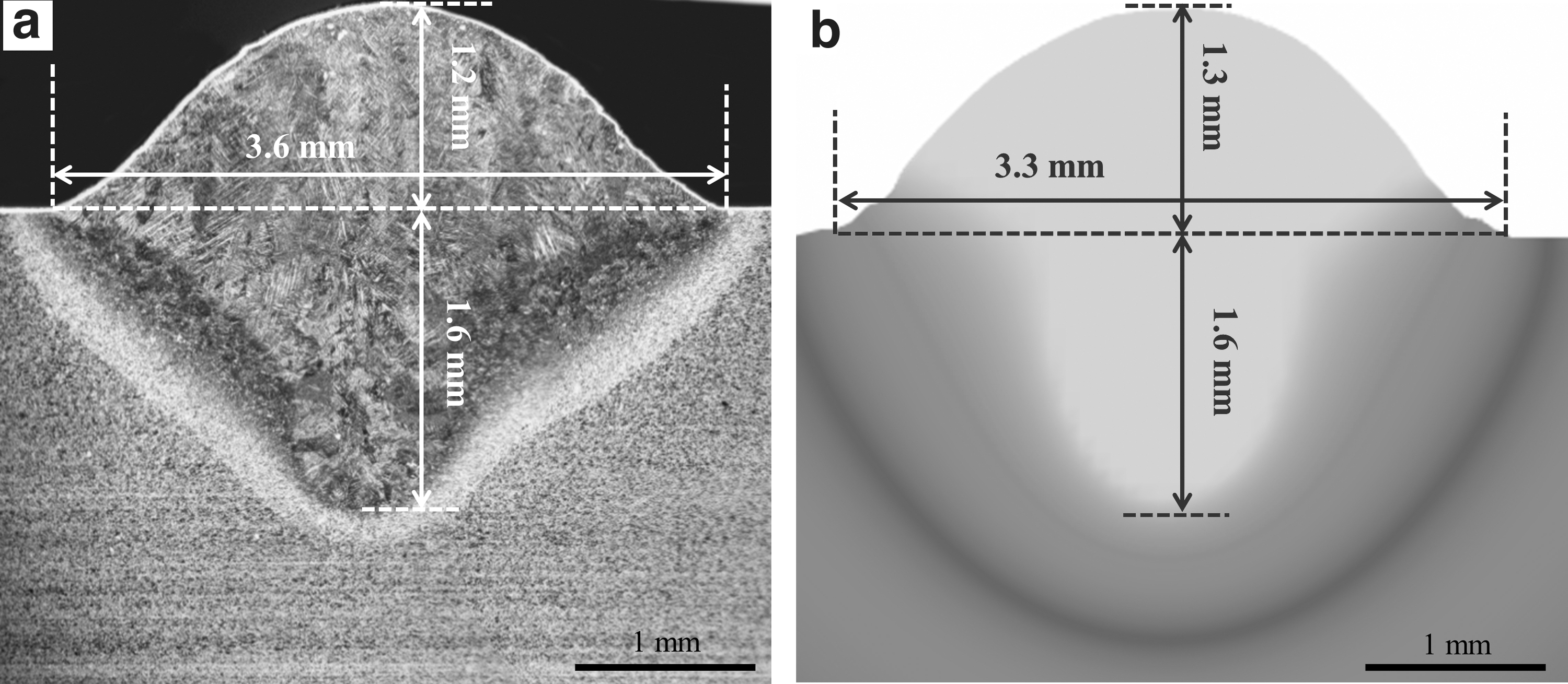
Comparing the experimental and simulation results of the cross-section of the deposition layer, (a) experimental result and (b) simulation result.

Discussion

The effect of recoil pressure on the morphology of deposited layer

As described in Experimental and Simulation section, the Marangoni flow, buoyancy flow, and recoil pressure were key factors affecting the flow of the molten pool. The marangoni flow and buoyancy flow were mainly determined by the temperature gradient. In addition, the flow of the molten pool was determined by the recoil pressure when the temperature was very high. In addition, Torkamany et al.⁴ showed that the recoil pressure was the main driving force to drive the flow of molten metal downward from the tip of the wire in the liquid bridge transfer mode.

To verify the role of recoil pressure in liquid bridge transfer behavior, a contrast simulation test was designed, in which the effect of recoil pressure was ignored and other process parameters remained unchanged. The results of contrast simulation test is presented in Figure 7, the width of the deposition layer was ∼1.2 mm. In addition, no layer was formed, which was consistent with the experimental results. Without considering the recoil pressure, the molten metal at the tip of the wire was difficult to separate from the wire. In addition, there was no keyhole in front of the molten pool, so the molten metal lacked the dynamic to flow. It indicated that the molten metal was difficult to spread to both sides of deposition layer only by marangoni flow and buoyancy flow.

FIG. 7.

CFD simulation results of the deposited layer morphology when ignoring the recoil pressure in the process of LWDed Ti-6Al-4V alloy. (a) t = 0.1 s; (b) t = 0.15 s; (c) t = 0.2 s.

Comparing with Figure 5a to d, it can be seen that under the action of recoil pressure, the molten metal at the tip of the wire was easily peeled off from the wire and enters the molten pool. In addition, the effect of keyhole dynamics on the molten pool gave the initial velocity of the molten metal, which made it easier to spread to both sides and form a deposition layer with good morphology. The contrast test showed that in the liquid bridge transfer mode, the recoil pressure promoted the spread of molten metal to both sides of deposition layer. Moreover, recoil pressure could not only peel off the molten metal from the tip of the wire and ensure stability of liquid bridge transfer but also promoted the flow of molten metal to both sides of the deposition layer and produced a well-formed deposition layer.

Flow behavior of molten pool

Figure 8 presents the CFD simulation of the morphology evolution and temperature distribution of the longitudinal section of the deposition center (y = 0 mm) at different times in the process of LWDed Ti-6Al-4V alloy. Red represents the molten pool in the temperature distribution diagram. When t was in the time range of 0–0.15 s, the depth of the molten pool increased gradually. However, when t was more than 0.15 s, the depth of the molten pool tended to be stable. In addition, the stable depth of molten pool was ∼1.6 mm. At the beginning of deposition, the molten metal solidified rapidly after contact with the substrate because there was no thermal accumulation, which played a supporting role to the subsequent molten metal, and made it difficult to flow to the rear.

FIG. 8.

CFD Simulation of the morphology evolution and temperature distribution of the longitudinal section of the deposition center (y = 0 mm) in the process of LWDed Ti-6Al-4V alloy at different time, (a) t = 0.1 s; (b) t = 0.15 s; (c) t = 0.2 s; (d) t = 0.25 s; (e) t = 0.3 s; (f) t = 0.35 s; (g) t = 0.4 s.

As a consequence, the height of the deposition layer increased rapidly with the increase of deposition metal volume, as shown in Figure 8a and b. The volume of the molten pool increased with the continuous accumulation of deposition metal. Then the flow range of molten metal gradually expanded. Under the effect of the molten pool flowing, wedge transition zone was gradually formed behind the keyhole, as shown from Figure 8c to g.

Hu et al.^10,25 studied the fluid dynamic of the liquid bridge transfer during the wire feeding 3D printing. Their study²⁵ found that the maximum magnitude of the flow speed was ∼2 m/s. Our simulation result showed that the maximum magnitude of the flow speed was ∼2.3 m/s. In addition, Hu et al.¹⁰ claimed that the dominant flow pattern of liquid bridge transfer was the molten metal flow from the wire tip to the molten pool through the liquid bridge, and the fluid in the molten pool flow to the rear part and sides by calculating the flow pattern on the surface of the molten pool. However, they ignored the flow pattern at the bottom of the molten pool.

Figure 9 is the flow streamline and the corresponding velocity distribution of the CFD-simulated molten pool at different times. Figure 9a and e revealed that at the beginning of deposition, there was less metal in the molten pool. In addition, the streamline of the molten pool flows from the bottom of the molten pool to the top surface. Figure 9b and f indicated that the increase of molten pool volume promoted the metal flow to the rear of the molten pool and formed an oval flow recirculation. Figure 9c and g showed that the tendency of metal flow toward molten pool rear became more obvious with further increase in the volume of the molten pool, resulting in a larger oval flow recirculation.

FIG. 9.

CFD simulation results of flow streamline (a–d) and the corresponding velocity distribution of the molten pool at different times (e–h). (a, e) t = 0.1 s (b, f) t = 0.2 s; (c, g) t = 0.3 s; (d, h) t = 0.4 s.

In addition, the angle between the long axis of the flow recirculation (shown in the red dotted line in the figure) and the laser scanning direction gradually increased. In Figure 9d and h, the angle between the long axis of the flow recirculation and the laser scanning direction further increased. Furthermore, the melt in the center of the oval flow recirculation were in a stationary state, indicated that the metal at the bottom of the molten pool mainly flowed toward the rear. In addition, the flow state tended to be stable. The molten metal flows toward the rear, resulting in volume reduction of the molten metal near the keyhole. Figure 8e to h show that the closer the distance to the keyhole was, the greater the flow velocity of the melt was. In addition, the greater the flow velocity was, the larger the volume of melt that flowed out per unit time was.

As a consequence, closer to the keyhole, the greater the volume of backward flow of molten metal, resulted in a decrease in the height of the deposited metal near the keyhole, which explained the formation mechanism of the wedge transition zone.

In the process of LWD, the height of the deposit metal was gradually reduced since the existence of wedge transition zone near the keyhole. At the end of the deposition, metal in the transition zone retained the original melt morphology, resulting in a decrease in the height of the tail of the deposition layer, as shown in Figure 5e. This explained the cause of the collapse at the tail of the deposition layer in the process of LWD. The mechanism of the wavy stripe could be clarified by Figures 8 and 9; the solidification direction of the deposition represented a certain angle with the laser scanning direction. It could deduce that the backward flow molten metal covered the prior solidified metal, and this molten metal retained the shape of the flow after solidification. In addition, it finally formed wavy stripes.

The effect of shielding effect of metal nanoparticles on the morphology of deposited layer

Figure 10 presents the CFD simulation of the morphology evolution and temperature distribution of the longitudinal section of the deposition center (y = 0 mm) when ignoring the shielding effect of metal nanoparticles on laser energy in the process of LWDed Ti-6Al-4V alloy. Red represents the molten pool in the temperature distribution diagram. Without considering the shielding effect of metal nanoparticles, the depth of the molten poll was ∼2.1 mm, which was about 0.5 mm higher compared with considering the shielding effect of metal nanoparticles. Comparing Figures 8 and 10, a hump was formed at the starting position of the deposited layer when ignoring the shielding effect of metal nanoparticles, and the maximum height of the hump was ∼2 mm.

FIG. 10.

CFD Simulation of the morphology evolution and temperature distribution of the longitudinal section of the deposition center (y = 0 mm) when ignoring the shielding effect of metal nanoparticles on laser energy in the process of LWDed Ti-6Al-4V alloy, (a) t = 0.1 s; (b) t = 0.15 s; (c) t = 0.2 s; (d) t = 0.25 s; (e) t = 0.3 s; (f) t = 0.35 s; (g) t = 0.4 s.

Figure 11 is the flow velocity distribution of the CFD-simulated molten pool when ignoring the shielding effect of metal nanoparticles on laser energy in the process of LWDed Ti-6Al-4V alloy. The maximum magnitude of the flow speed was ∼3.5 m/s, which was about 1.2 m/s higher compared with considering the shielding effect of metal nanoparticles. Comparing Figures 9 and 11, the molten metal tended to flow toward the tail of the deposited layer without considering the shielding effect of metal nanoparticles, thus forming a hump. Metal nanoparticles have attenuation effects such as absorption, reflection, and scattering of laser beam.¹¹

FIG. 11.

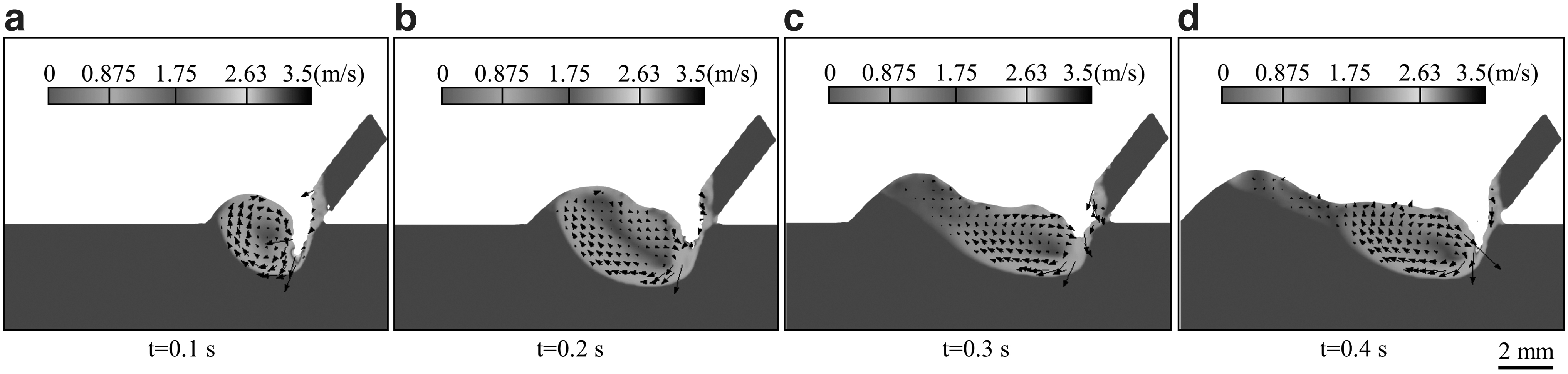
CFD simulation results of flow velocity distribution of the molten pool when ignoring the shielding effect of metal nanoparticles on laser energy in the process of LWDed Ti-6Al-4V alloy. (a) t = 0.1 s (b) t = 0.2 s (c) t = 0.3 s (d) t = 0.4 s.

Regardless of the shielding effect of nanoparticles on the laser, the energy absorbed in the molten pool increased. It could be seen from the recoil pressure model that the higher the energy absorbed by the molten metal, the greater the recoil pressure of the molten metal. That was, a larger flow velocity can be obtained, which increased the velocity of the melt flow backward.

Thermal performance of molten pool

David et al.²⁶ pointed out that the solidification behavior determined the grain size and morphology during the liquid to solid transformation. The key factors determining the solidification structure were molten pool temperature gradient G, solidification rate R, supercooling, and alloy composition. The solidification morphology changed to cellular, columnar, and equiaxed grains with the increase of R. And the fine solidification structure would be produced. Zhong and Liu²⁷ believed that the cooling rate of laser AM usually varies from 10² to 10⁶ K/s.

Kobryn and Semiatin²⁸ drew the solidification map of Ti-6Al-4V alloy by temperature gradient (G) and solidification growth rate (R), to predict the morphology of solidification structure. However, it is difficult to measure G and R in experiment due to the melt convection in the molten pool. As a consequence, it is a great method for alternative experimental measurements of G and R by using numerical simulation, which includes heat transfer and fluid convection.²⁹

G and R were extracted from the melt pool boundary by the method of Lee et al.³⁰ The temperature gradient vector G was perpendicular to the solid-liquid interface of the molten pool and could be decomposed into three components: G_x, G_y, and G_z. These components could be obtained directly from the simulated temperature distribution at the boundary of the molten pool. In addition, Equation (18) was used to calculate the temperature gradient G at the front of solidification. $G = \sqrt{G_{x}^{2} + G_{y}^{2} + G_{z}^{2}}$ (18)

The temperature gradient distribution on the solidification boundary of the molten pool is shown in Figure 12. According to the temperature gradient distribution map, it could be seen that from the front of the molten pool to the rear of the molten pool, the temperature gradient presented a downward tendency. And from the bottom of the molten pool to the top of the molten pool, the temperature gradient showed an upward tendency. Furthermore, the maximum value of the temperature gradient of the molten pool was ∼2050 K/mm, and the minimum value was ∼600 K/mm under the conditions of this study. In addition, the average value was ∼1100 K/mm.

FIG. 12.

Temperature gradient distribution at the boundary of the molten pool. The above illustration shows the location of data points on the three-dimensional graph of the molten pool solidification boundary. The below illustration shows the temperature gradient cloud map fitted according to data points.

The solidification rate R on the solid-liquid interface was related to the laser scanning speed v and the angle θ between the solid-liquid interface and the laser scanning direction. R was obtained by Rappaz et al.³¹: $R = cos (θ) v$ (19)

where cos( $θ$ ) can be expressed with Equation (20): $cos (θ) = G_{X}^{2} ∕ G$ (20)

The solidification velocity distribution of the solidification boundary is shown in Figure 13. The solidification velocity distribution tendency was different from the temperature gradient distribution trend. The solidification velocity of the molten pool boundary showed that the fast solidification area was at the front and rear of the molten pool and slow solidification area was at the middle of the molten pool. The region with the fastest solidification speed was located at the bottom of the molten pool. The maximum solidification rate of the molten pool was ∼20 mm/s, and the minimum was ∼1.5 mm/s under the conditions of this study. In addition, the average value of solidification speed was ∼10 mm/s.

FIG. 13.

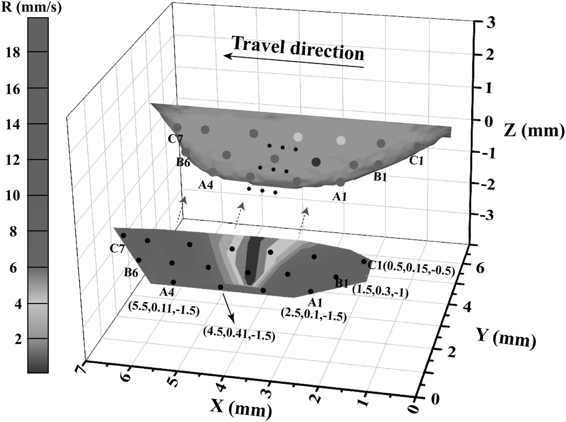
Distribution of grain growth rate at the boundary of molten pool. The above illustration shows the location of data points on the three-dimensional graph of the molten pool solidification boundary. The below illustration shows the temperature gradient cloud map fitted according to data points.

The cooling rate of the molten pool boundary C is expressed in Equation (21): $C = G \cdot R$ (21)

The cooling rate distribution of the solidification boundary is shown in Figure 14. The distribution tendency of cooling rate was similar to that of solidification speed, the fast cooling rate area was at the front and rear of the molten pool and slow cooling rate area was at the middle of the molten pool. The fastest cooling rate area was located at the front of the molten pool. The maximum solidification rate of the molten pool was ∼3000 K/s, and the minimum value was ∼1100 K/s under the conditions of this study. In addition, the average value of cooling rate was ∼11,000 K/s.

FIG. 14.

Distribution of cooling rate at the boundary of the molten pool. The above illustration shows the location of data points on the three-dimensional graph of the molten pool solidification boundary. The below illustration shows the temperature gradient cloud map fitted according to data points.

Conclusion

A three-dimensional CFD model of the interaction between laser and Ti-6Al-4V alloy wire and Ti-6Al-4V alloy substrate was established and verified by experimental results. The melting of wire and forming process of deposition layer at the mesoscale were revealed by the model and the main conclusions are as follows: (1)

The dynamic behavior of fluid metal in the process of liquid bridge transfer was simulated by LWD CFD. In addition, the simulation results were in good agreement with the experimental results.

(2)

Recoil pressure ensured that the deposited metal spread to both sides of deposition layer in the liquid bridge transfer model. The molten metal at the wire tip was peeled and entered the molten pool under recoil pressure. Under the effect of keyhole dynamics in molten pool, the initial speed of spreading to both sides of deposition layer was obtained.

(3)

The backward flow of molten metal, resulting in the metal volume reduction near the keyhole and formation a wedge-shaped transition zone. The morphology of deposition layer tail maintained the shape of the wedge transition zone after the end of the deposition because there was no replenishment of molten metal, which lead the tail of the deposition layer was easy to collapse in the process of LWD.

(4)

The simulation results showed that the temperature gradient of the molten pool boundary was ∼1100 K/mm, and the solidification rate was ∼10 mm/s. In addition, the cooling rate was ∼11,000 K/s under the conditions in this study.

Footnotes

Acknowledgments

The authors thank the teachers at the Instrument Analysis Center of Xi'an Jiaotong University for their assistance with the SEM and EBSD analysis.

Author Disclosure Statement

No competing financial interests exist.

Funding Information

This work was supported by the National Key Research and Development Project of P.R. China (Grant No. 2018YFB1105803) and National Thousand Talents Program of P.R. China (Grant No. WQ2017610446). This work was also supported by the Project of Innovation Team of Xi'an Jiaotong University (Grant No. XTR0118008).

References

Matthews

, Guss

, Khairallah

, et al. Denudation of metal powder layers in laser powder bed fusion processes. Acta Mater, 2016; 114:33–42.

, Han

, Fang

, et al. Mechanism of surface morphology in electron beam melting of Ti6Al4V based on computational flow patterns. Appl Surf Sci, 2017; 419:150–158.

Bai

, Colegrove

, Ding

, et al. Numerical analyswas of heat transfer and fluid flow in multilayer deposition of PAW-based wire and arc additive manufacturing. Int J Heat Mass Transf, 2018; 124:504–516.

Torkamany

, Kaplan

AFH

, Ghaini

. Wire deposition by a laser-induced boiling front. Opt Laser Technol, 2015; 69:104–112.

, Huang

, Wang

. Investigation of melting dynamics of filler wire during wire feed laser welding. J Mec Sci Technol, 2013; 27:1097–1108.

, Li

, Chen

. Effects of beam confgurations on wire melting and transfer behaviors in dual beam laser welding with fller wire. Opt Laser Technol, 2017; 91:138–148.

Abioye

, Folkes

, Clare

. A parametric study of Inconel 625 wire laser deposition. J Mater Process Tech, 2013; 213:2145–2151.

Wei

, Wang

, Shin

, et al. Comprehensive modeling of transport phenomena in laser hot-wire deposition process. Int J Heat Mass Transf, 2018; 125:1356–1368.

, Li

. Computational fluid dynamic simulation of gravity and pressure effects in laser metal deposition for potential additive manufacturing in space. Int J Heat Mass Transf, 2019; 140:51–65.

10.

, Luo

, Liu

, et al. Thermal fluid dynamics of liquid bridge transfer in laser wire deposition 3D printing. Sci Technolf Weld Join, 2019; 24:1–11.

11.

Chatterjee

, Chakraborty

. A hybrid lattice Boltzmann model for solid–liquid phase transition in presence of fluid flow. Phys Lett A, 2006; 351:359–367.

12.

, Cheon

, Kiran

, et al. CFD simulations of GMA welding of horizontal fillet joints based on coordinate rotation of arc models. J Mater Process Tech, 2016; 231:221–238.

13.

Gerhard

, Boyer

, Collings

. Materials Properties Handbook: Titanium Alloys. ASM International: Almere, The Netherlands, 1994.

14.

Colegrove

, Simiand

, Varughese

, et al. Evaluation of a drilling model approach to represent laser spot microwelding. In: ASM Proceedings of the international conference: trends in welding research; 2009.

15.

Boivineau

, Cagran

, Doytier

, et al. Thermophysical properties of solid and liquid Ti-6Al-4V (TA6V) alloy. Int J Thermophys, 2006; 27:507–529.

16.

Shejndlin

, Kenisarin

, Chekhovskoj

. Melting point of yttrium oxide. AN SSSR, 1974; 216:582–584.

17.

Cho

, Na

. Teflection and Fresnel absorption of laser beam in keyhole. J Phys D Appl Phys, 2006; 39:5372–5378.

18.

Han

, Ahn

, Na

. A study on ray tracing method for CFD simulations of laser keyhole welding: Progressive search method. Weld World, 2016; 60:247–258.

19.

Allmen

MV.

Laser-Beam Interactions with Materials. Springer, Berlin-Heidelberg, 1995.

20.

Dobson

. Absorption and scattering of light by small particles. Phys Bull, 1984; 35:104.

21.

Greses

, Hilton

, Barlow

. Plume attenuation under high power Nd:yttritium aluminum garnet laser welding. J Laser Appl, 2004; 16:9–15.

22.

Shcheglov

, Uspenskiy

, Gumenyuk

, et al. Plume attenuation of laser radiation during high power fiber laser welding. Laser Phys Lett, 2011; 8:475–480.

23.

Yang

, Liou

. Effective refractive index for determining ray propagation in an absorbing dielectric particle. J Quant Spectrosc Radiat Transf, 2009; 110:300–306.

24.

Barber

. Absorption and scattering of light by small particles. J Colloid Interface Sci, 1984; 98:290–291.

25.

, Chen

, Yang

, et al. Metal transfer in wire feeding-based electron beam 3D printing: Modes, dynamics, and transition criterion. Int J Heat Mass Transf, 2018; 126:877–887.

26.

David

, Babu

, Vitek

. Welding: Solidification and microstructure. JOM, 2013; 55:14–20.

27.

Zhong

, Liu

. Laser surface cladding: The state of the art and challenges. Proc Inst Mech Eng Part C J Mech Eng Sci, 2010; 224:1041–1060.

28.

Kobryn

, Semiatin

. Microstructure and texture evolution during solidification processing of Ti-6Al-4V. J Mater Process Technol, 2003; 135:330–339.

29.

Debroy

, David

. Physical processes in fusion welding. Rev Mod Phys, 1995; 67:85–112.

30.

Lee

, Nordin

, Babu

, et al. Effect of fluid convection on dendrite arm spacing in laser deposition. Metall Trans B, 2014; 45:1520–1528.

31.

Rappaz

, David

, Vitek

, et al. Development of microstructures in Fe15Ni15Cr single crystal electron beam welds. Metall Trans A, 1989; 20:1125–1138.