Automated Defect Recognition for Additive Manufactured Parts Using Machine Perception and Visual Saliency

Abstract

Metal additive manufacturing (AM) is known to produce internal defects that can impact performance. As the technology becomes more mainstream, there is a growing need to establish nondestructive inspection technologies that can assess and quantify build quality with high confidence. This article presents a complete, three-dimensional (3D) solution for automated defect recognition in AM parts using X-ray computed tomography (CT) scans. The algorithm uses a machine perception framework to automatically separate visually salient regions, that is, anomalous voxels, from the CT background. Compared with supervised approaches, the proposed concept relies solely on visual cues in 3D similar to those used by human operators in two-dimensional (2D) assuming no a priori information about defect appearance, size, and/or shape. To ingest any arbitrary part geometry, a binary mask is generated using statistical measures that separate lighter, material voxels from darker, background voxels. Therefore, no additional part or scan information, such as CAD files, STL models, or laser scan vector data, is needed. Visual saliency is established using multiscale, symmetric, and separable 3D convolution kernels. Separability of the convolution kernels is paramount when processing CT scans with potentially billions of voxels because it allows for parallel processing and thus faster execution of the convolution operation in single dimensions. Based on the CT scan resolution, kernel sizes may be adjusted to identify defects of different sizes. All adjacent anomalous voxels are subsequently merged to form defect clusters, which in turn reveals additional information regarding defect size, morphology, and orientation to the user, information that may be linked to mechanical properties, such as fatigue response. The algorithm was implemented in MATLAB™ using hardware acceleration, that is, graphics processing unit support, and tested on CT scans of AM components available at the Center for Innovative Materials Processing through Direct Digital Deposition (CIMP-3D) at Penn State's Applied Research Laboratory. Initial results show adequate processing times of just a few minutes and very low false-positive rates, especially when addressing highly salient and larger defects. All developed analytic tools can be simplified to accommodate 2D images.

Introduction

Significant resources are required to properly evaluate part quality using nondestructive inspection tools such as X-ray computed tomography (CT) scans. Especially for additively manufactured (AM) parts, material integrity and thus part quality cannot always be guaranteed. In fact, discontinuities (or flaws) in the resultant component commonly arise as a result of abnormal part solidification or due to process deviations from the nominal build environment.^1,2 As noted in Yavari et al.³ and Liu et al.,⁴ the number, size, and morphologies of the resulting flaws can be linked to the structural integrity of the melted material and ultimately to part quality.

Currently, trained professionals are needed to certify the part quality by virtue of manual evaluation of CT scans, which is a labor- and cost-intensive process. In addition, perceived defect severities and morphologies, which hold valuable information regarding material properties and the structural integrity of the part, may often be subjective and thus inconsistent between evaluators. To close this technological gap, we present and validate a complete solution for three-dimensional (3D) automated defect recognition (ADR) using CT scans.

Although commercial ADR algorithms exist, the algorithms are proprietary and therefore closed, have results that are strongly influenced by manual settings, and do not provide detailed flaw morphology information that is critical for certain kinds of analysis (i.e., mapping in situ sensor data collected during an AM build to actual flaws in the final part). Although the algorithm was initially developed for AM parts, it is applicable to any part or material that can be CT scanned. All developed analytic tools can be simplified to accommodate two-dimensional (2D) images.

As described in Spierings and Schneider and Wits et al.,^5,6 the commonly used techniques for postbuild inspection include Archimedes' method and ultrasonic inspection (both nondestructive), as well as the evaluation of micrographs of cross sections (destructive). Archimedes' method is a density measurement approach that links the assumed material density and the measured part density, that is, measured weight per volume, to part porosity. Although “the resulting porosity metric is regarded as important quality indicator in metal AM,” Archimedes' method provides no additional information regarding defect sizes, number, or locations.

On the contrary, micrographs of cross sections allow for a very detailed assessment of defect morphologies. The fidelity of the assessment is a function of magnification, the preparation process for the cross section, as well as available analysis tools. However, micrograph assessment is labor-intensive and restricted to just a few local regions, that is, slices, for which micrographs can be obtained and evaluated. Defect statistics for those small, local regions can subsequently be extrapolated across the entire part to approximate the overall porosity using techniques such as the Scheil–Saltykov correction method described in Gegner.⁷ Clearly, the latter assumes a rather uniform morphology and distribution of defects, that is, location and size, across the entire part, which may not always be the case.

An overview of the current state-of-the-art in CT is provided in du Plessis et al.⁸ and Baniukiewicz.⁹ An overall background on X-ray imaging, including parameter choices and their impact on the resulting CT image, is provided. Specifically, the authors of du Plessis et al.⁸ establish the fundamental correlation between perceived CT intensities, that is, the X-ray return amplitude, and material density, which ultimately lays the groundwork for CT-based porosity and defect detection. Therefore, it is proposed that X-ray CT inspection and data analysis should be a crucial part of any holistic quality control for AM. However, a high level of automation will be required for consistency and high-confidence CT evaluation and to avoid logistical bottlenecks.

For automated defect detection, one generally distinguishes between supervised and unsupervised classification techniques. The first assumes a set of labeled data that can be utilized to generate a decision boundary between the classes in a higher dimensional feature space. The latter attempts to derive such decision boundaries based on the statistical distribution and spread of available data samples without explicit labels. Supervised classification is carried out in Hou et al.¹⁰ for welding defects using a neural network architecture, and in Mery and Arteta¹¹ for defect detection in automotive parts while comparing a variety of classifications schemes. Although supervised techniques may achieve accuracies of 90%, classification performance is often dependent on the quantity and quality of available training samples.

In Hou et al.¹⁰ and Mery and Arteta,¹¹ data sets of 32 × 32 image tiles are provided that have been labeled manually as either “defect” or “no defect.” In contrast, in this study, defects are identified in an unsupervised manner using visual saliency as a discriminator. Since its inception in Itti and Koch,¹² visual saliency has been defined as “the distinct subjective perceptual quality which makes some items in the world stand out from their neighbors and immediately grab our attention.”

Therefore, our approach does not require training samples, which are often difficult and expensive to obtain and label, and there is no assumption regarding the morphology and/or size of the defects. In addition, defect detection is carried out in 3D compared with 2D to fully evaluate CT intensity changes as well as local minima/maxima in all directions. As a consequence, the algorithm is inherently agnostic to the orientation of the part during CT scanning and/or the direction of individual 2D CT slices. Most importantly, our algorithm may accommodate potentially billions of CT voxels and still achieve a reasonable run-time of just 2 min.

Defect detection based on 2D image segmentation is carried out in Faiza and Nacereddine¹³ and Lawson and Parker.¹⁴ During image segmentation, adjacent pixels with similar attributes, in this study, CT intensity, are combined into larger segments or superpixels. In Faiza and Nacereddine,¹³ features such as compactness, elongation, and/or eccentricity can be computed for each superpixel, and classification can be carried out based on those derived features. In contrast, the work in Faiza and Nacereddine¹³ utilizes a neural network for segmentation-based defect detection. Both methods rely on computing similarities between any pixel and its neighbors in a 4-connected or 8-connected sense, which is computationally tractable for most 2D images. However, given 3D imagery data, such as provided by CT scans, neighbor similarities must be computed in a 6-, 18-, or 26-connected sense for potentially billions of voxels.

Therefore, we do not compute 26-connected voxel similarities explicitly but rather address local changes in CT intensity directly by establishing visual saliency using fast 3D convolution operations.

Difficulties for ADR through CT scans often arise due to the so-called beam-hardening effects¹⁵ and scattered radiation.^16,17 Beam-hardening describes the process in which the lower frequency (lower energy) portions of a polychromatic X-ray beam are preferentially attenuated as the aggregate beam penetrates the material. As a result, the beam that reaches the interior of the part comprises a greater proportion of higher frequency bands, diminishing the effective attenuation coefficient of those regions of the part. Since the CT reconstruction process produces a map of the relative attenuation coefficients of the part on a voxel-wise basis, the interior appears darker (less attenuating) in the resulting CT scan compared with the regions near the edge. Figure 1 illustrates the beam-hardening effect using an actual CT sample. CT intensities are shown as 2D image (upper left) and surface plot (lower graph).

FIG. 1.

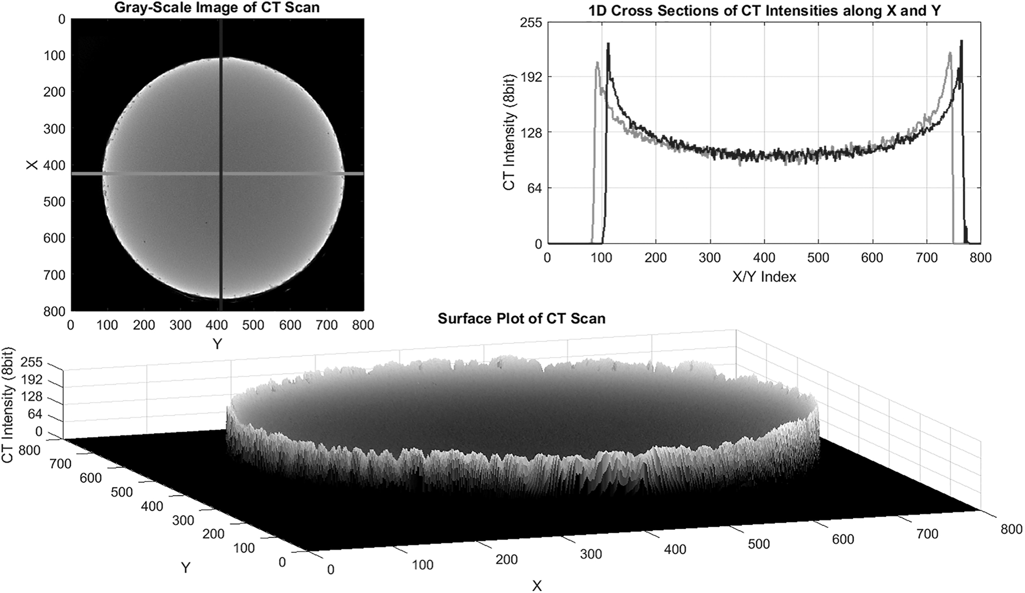
Illustration of beam-hardening effect using an actual CT sample. CT intensities are shown as gray-scale image (upper left) and surface plot (lower graph). The upper right shows the CT intensities as cross sections along the red and blue lines. CT, computed tomography.

In addition, cross sections of CT intensities are shown along the red and blue lines (upper right). As one can see, recorded CT intensities decrease significantly away from the edges.

Scattering of the incident X-ray beam describes the process through which an incoming photon interacts with orbital electrons of the examination object's atoms, resulting in the photon being deflected from its original vector.¹⁶ The result is that the photon contributes to signal at an element of the digital detector that is inconsistent with the X-ray transmission geometry that is assumed for reconstruction. The impact on the CT data can be the appearance of streaks in the images¹⁷ around highly attenuating objects. In the present case, we consider nominally homogeneous objects, where the primary impact of scatter is to increase the overall noise level, or “randomness,” of the gray-value intensities because of the numerous contributions to signal at random locations in the field of view. The result is an overall diminishing of contrast within the data set.

Although beam hardening and scatter can be reduced through both hardware and software solutions,¹⁸ each of these solutions comes at its own cost, and often cannot completely eliminate the image artifacts. Therefore, ADR based on intensity alone, that is, through simple thresholding, is not considered a feasible approach. Instead, CT intensities, and changes therein, must therefore be evaluated with respect to CT intensity values within a local region.

The article is organized as follows. The Technical Approach section describes the technical approach, including the automated extraction of the part boundary in the Extracting the Part Boundary and Generating the Mask section, the generation of visual saliency in the Generating Visual Saliency section, and the extraction of CT anomaly voxels in the Extracting CT Anomalous Voxels section. The approach is validated in the Experimental Validation section using the existing CT scans. Detected defects are manually inspected to separate true positives (TPs) from false positives (FPs), and performance metrics are derived to assess algorithm performance for various saliency levels. Conclusions are presented in the Conclusion section, while the Future Work section outlines future work.

Technical Approach

This section outlines the technical approach as a complete tool chain that ingests the raw CT image stack in three dimensions and outputs a list of CT anomaly clusters with corresponding attributes, that is, perceived saliency, size, morphology, and orientation.

The Extracting the Part Boundary and Generating the Mask section describes the extraction of the part boundary, that is, the separation of part voxels and background voxels, using statistical measures. This allows the algorithm to be applied to any part geometry without the need for additional part information or CAD files. The part boundary is converted into a 3D binary mask that guides the anomaly detection. The Generating Visual Saliency section focuses on the extraction of CT anomalies within the part. Machine perception and image processing concepts such as visual saliency are generalized, scaled, and applied to the three-dimensional CT voxel data. As a result, individual voxels are flagged as either anomalous or nominal. As the last step, the Extracting CT Anomalous Voxels section discusses a method to merge adjacent anomaly voxels into clusters. Clusters may then be analyzed for severity of the defect as deduced from the resulting CT intensity gradient as well as perceived size, shape, and orientation.

Extracting the part boundary and generating the mask

To confine the ADR to the actual part and avoid false detection near the edge of the part or in the background, a binary mask is generated. As shown in Figure 2, the material generally separates itself from the background through higher CT intensity values. In this case, the cylindrical test coupon (∼10 mmø × 25 mm) was built using metal powder bed fusion AM on a 3D Systems ProX 320 using the standard Ti6Al4V powder and processing recipe, with CT scan parameters set to produce a voxel size of 15 μm.

FIG. 2.

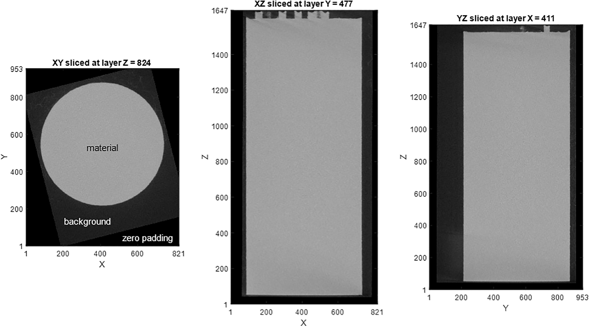
Two-dimensional slices of the raw 3D CT scan showing XY slice, XZ slice, and YZ slice from left to right. CT intensities are commonly encoded as gray-scale values using 8- or 16-bit unsigned integers. 2D, two dimensional; 3D, three dimensional.

We define the CT intensity at location $r = {[x, y, z]}^{T}$ as $I (r) \in ℛ$ (1)

The CT intensity $I (r)$ is often provided as an 8-bit, a 12-bit, or a 16-bit integer value. Furthermore, we define $h (I)$ to be the histogram over all intensity values within the CT image stack. The histogram $h (I)$ can be used to separate the regions of low- and high-intensity X-ray returns, that is, the material from the background. Specifically, we use a Gaussian mixture model (GMM)¹⁹ to represent $h (I)$ and select two mixtures (or components), one for the material intensities and one for the background

Here, $μ_{i}, σ_{i}$ are the respective mean and standard deviation of component i, and $ϕ_{i}$ is the corresponding mixture weight. Software libraries exist to optimize the GMM fit (2) using, for example, Expectation Maximization tools. Figure 3 shows $h (I)$ as well as the corresponding GMM components using the CT scan data shown in Figure 2. The two distinct CT intensity distributions for background (low values, green line) and part (higher values, red line) are clearly visible. A threshold for separating material from background, as indicated by the magenta line, can be found where the expectations of both components are equal. Manually decreasing/increasing the proposed threshold dilates/erodes the binary “part” mask for ADR.

FIG. 3.

Histogram of CT intensities (blue) using a 16-bit unsigned integer representation, that is, [0, 65535]. The Gaussian mixture components for background and material are shown in green and red, respectively. A threshold for separation can be found where the expectations of both components are equal, see magenta line.

If needed for computational reasons, the histogram $h (I)$ may be approximated using only a subset of all $x, y, z$ locations. In fact, the CT scan from Figure 2 consists of 1,288,634,221 data points, which may render the GMM approach infeasible to execute in reasonable time. Several tests have shown that randomly downsampling the number of data points used to generate the histogram by several orders of magnitude, here a factor of 1000, does not significantly alter the resulting threshold, while speeding up the computation significantly.

In addition, it is important to note that the GMM approach outlined above labels individual voxels as material or background using the expectations of the two GMM components. Material voxels may or may not form one connected cluster. In fact, multiple, disconnected clusters may form specifically around the edge of the part. Similarly, large defects with low CT intensity in the interior of the part may be labeled as background, which in turn will exclude them from the subsequent ADR algorithm. It is therefore recommended to apply 3D Gaussian smoothing to the entire CT scan²⁰ before constructing the GMM to blur out some of those inclusions. Convolution kernels that are twice the size of those used for ADR have shown the best results.

Any remaining background clusters that are fully enclosed by the material cluster may be discarded and merged back into the mask. Figure 4 shows the binary mask resulting from the CT intensity separation through the GMM.

FIG. 4.

Resulting binary mask for ADR. The mask is generated using a GMM to separate material from background based on the CT intensity values of the smoothened image. ADR, automated defect recognition; GMM, Gaussian mixture model.

Let $ϒ$ be the volume of the part as indicated by the mask and $\bar{ϒ}$ its complement, that is, all background voxels, with $ϒ \cap \bar{ϒ} = \emptyset$ . Then, we define an exterior distance function $d_{ϒ}^{p} (r)$ with respect to the surface of the part as follows:

Here, the superscript p denotes the $ℒ_{p}$ -norm used. Note, we define $d_{ϒ}^{p} (r) = 0$ for any point inside the part, that is, $r \in ϒ$ . Similarly, the interior distance function is defined as follows:

with $d_{\bar{ϒ}}^{p} (r) = 0$ for any point outside the part, that is, $r \in \bar{ϒ}$ . For the sake of compatibility, both quantities $d_{ϒ}^{p} (r)$ and $d_{\bar{ϒ}}^{p} (r)$ are measured in voxels. Units may be adjusted afterward using the actual CT scan resolution, commonly measured in microns per voxel.

Euclidean distance transform algorithms, such as those outlined in Maurer et al.²¹ enable efficient computations for both distances (3) and (4) for any binary mask over the entirety of the 3D CT domain. With subsequent convolution operations in mind, utilizing the $ℒ_{\infty}$ -norm, that is, $p = \infty$ , for (3) and (4) has been shown to be most advantageous. By definition, the $ℒ_{\infty}$ -norm represents the largest magnitude among each of the elements of a vector and thus captures the max distance of the point r to the volume $ϒ$ or $\bar{ϒ}$ in any of the three dimensions. Therefore, the $ℒ_{\infty}$ -norm is the most appropriate when attempting to slide the convolution kernel close to the edge of the mask. Following the conventions introduced in Morgan et al.²² we define the distance function $D^{\infty} (r)$ positive outside the part and negative inside. That is $D^{\infty} (r) = d_{ϒ}^{\infty} (r) - d_{\bar{ϒ}}^{\infty} (r)$ (5)

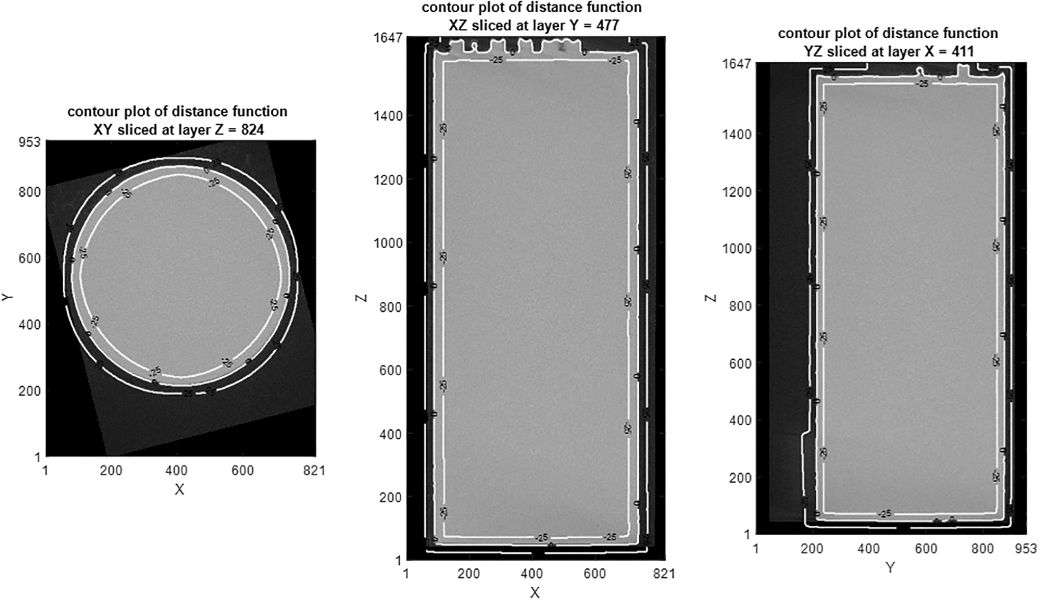
Figure 5 shows the CT scan from Figure 2 with contour lines for $D^{\infty} (r) = - 25, 0, + 25$ (measured in voxels) overlaid in yellow. As one can see, the contour line for $D^{\infty} (r) = 0$ follows the outline of the part with sufficient accuracy and thus provides adequate information for separating the part from the background for further analysis. To verify generality, the masking approach has been validated for several CT scans.

FIG. 5.

Two-dimensional slices of the raw 3D CT scan showing XY slice, XZ slice, and YZ slice from left to right. Contour lines for $D^{\infty} (r) = - 25, 0, + 15$ (measured in voxels) are overlaid in yellow.

A binary mask, $M_{λ} (r)$ , can now be defined by applying a threshold parameter, $λ$ (or mask margin), to the distance function $D^{\infty} (r)$ from Equation (5). Specifically, we define the following: $M_{λ} (r) = \{\begin{matrix} 1 & i f D^{\infty} (r) < λ \\ 0 & i f D^{\infty} (r) \geq λ \end{matrix}\}$ (6)

The mask may further be dilated or eroded by adjusting the corresponding threshold $λ$ for $D^{\infty} (r)$ . Slightly eroding the mask by just a few voxels (with λ < 0) is advantageous for ADR performance as it filters out residual classification errors (part vs. background) around the edge of the part stemming from the GMM thresholding. Dilating the mask (with λ > 0) allows the algorithm to detect near-edge defects, but will also increase the number of FPs wherever misalignment errors occur. Note that the largest intensity gradients are found at the edge of the part. Therefore, an overly dilated mask may cause the ADR algorithm to falsely interpret those gradients as defects.

Generating visual saliency

During CT analysis, indications often manifest themselves as voxels or local areas of low or high intensity compared with the surrounding material (Fig. 6). Anomalous CT voxels can be divided into two classes: (1) voids or pores, defined as low-intensity CT voxels surrounded by higher intensity CT voxels (see left side in Fig. 6) and (2) superdensities (perhaps as the result of powder contamination), which are high-intensity CT voxels surrounded by lower intensity CT voxels (see right side in Fig. 6). Nominal CT voxels, characterized by discontinuity and indication-free regions of a test part, are observed as CT voxels that are surrounded by similar intensity CT voxels, thereby generating a near-zero visual saliency.

FIG. 6.

Indications in CT scan showing (1) void or pore, characterized by low-intensity voxels, that is, local minimum (left) and (2) superdensity, characterized by high-intensity voxels, that is, local maximum (right).

To detect defects such as those shown in Figure 6, the overall saliency is established following machine perception and image processing concepts first outlined in Itti and Koch¹² and Niebur et al.²³ More recent variants and approaches can be found in Cong et al.²⁴ Specifically, visual attention is generated through saliency to identify voxels or regions that “stand out” in the local neighborhood.

Figure 7 outlines the overall concept for anomaly detection using convolution operations. Assuming a simplified, one-dimensional (1D) case, the CT intensity $I (x)$ (shown on the left) is convolved with a convolution kernel K (shown in the center plot) to extract local intensity minima. The resulting convolution response $R (x)$ is shown on the right. For this example, a threshold of −0.21 is chosen at −4 standard deviations from the mean response of $R (x)$ . The threshold is shown as a dashed black line in the right figure. Note that simply thresholding the CT intensity $I (x)$ in the left figure would not yield the desired results.

FIG. 7.

Simplified 1D concept for CT anomaly detection using a convolution operation to extract local intensity minima. 1D, one dimensional.

Without assuming any prior knowledge on defect formation, size, or morphology, the ADR algorithm utilizes a multiscale, 3D Gaussian kernel, K _n, to infer visual saliency. By design, the kernel is held fully symmetric and separable. Over the normalized 3D domain with $x_{k}, y_{k}, z_{k} \in [- 1, + 1]$ , we define K_n as follows: $K_{n} (x_{k}, y_{k}, z_{k}) = exp (- \frac{x_{k}^{2} + y_{k}^{2} + z_{k}^{2}}{σ_{k}^{2}}) - γ_{0} \in ℛ^{n \times n \times n}$ (7)

with standard deviation $σ_{k} = 0.5$ and scalar offset parameter $γ_{0} \in ℛ$ . The offset parameter is introduced to yield a zero mean kernel, that is,

By definition, the zero mean kernel (7) satisfying (8) will generate a visual saliency of zero when convolved over CT intensities that are constant.

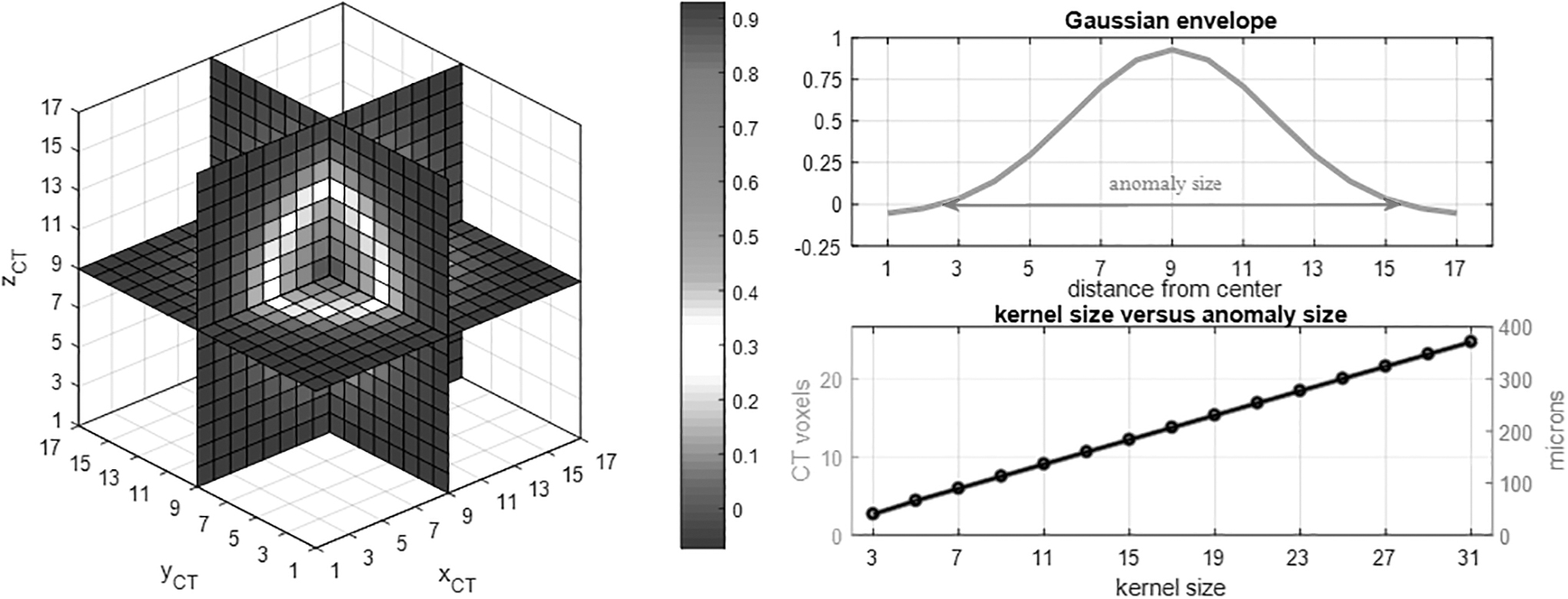
In Equation (7), n denotes the size of the kernel, which in turn dictates the spacing of $x_{k}, y_{k}, z_{k}$ over the normalized domain $[- 1, + 1]$ . In other words, the actual size of the normalized kernel (7) can be selected to extract anomalies of different physical sizes within the CT imagery. Therefore, the individual domains for $x_{k}, y_{k}$ and z_k will be discretized and subdivided into the appropriate number of CT voxels, n, which then defines the physical size of the 3D Gaussian kernel in voxels or microns. The left plot in Figure 8 shows a sliced view of such a kernel for $n = 17$ . Assuming a CT resolution of 15 μm per voxel, this kernel size corresponds to a volume of (255 μm)³.

FIG. 8.

Left—sliced view of 3D Gaussian kernel of size $n = 17$ used for anomaly detection in CT. Right—Gaussian envelope in 1D (top) and approximate anomaly size versus kernel size (bottom).

The right side of Figure 8 depicts the Gaussian envelop in 1D, which also illustrates the approximate size of the anomaly that would generate a strong correlation (or match) and thus be extracted by virtue of 3D image convolution. The lower plot shows the approximate size of extracted anomalies when using kernel sizes $n = 3$ up to $n = 31$ , again assuming a CT scan resolution of 15 μm per voxel. As larger kernels create a stronger correlation with larger anomalies, it is important to select a set of kernel sizes based on the anticipated defect sizes or the defect sizes of interest.

Compared with prior work outlined in Gobert et al.²⁵ in which a Gabor wavelet was used, a Gaussian kernel allows for the separation of dimensions during the convolution, which significantly reduces the computational complexity. In fact, it can be shown that any 3D convolution using the Gaussian kernel (7) can be separated using three 1D kernels as follows: $\begin{matrix} k_{x} = exp (- x_{k}^{2} ∕ σ_{k}^{2}) \in ℛ^{n \times 1 \times 1} \\ k_{y} = exp (- y_{k}^{2} ∕ σ_{k}^{2}) \in ℛ^{1 \times n \times 1} \\ k_{z} = exp (- z_{k}^{2} ∕ σ_{k}^{2}) \in ℛ^{1 \times 1 \times n} \end{matrix}$ (9)

The quantities k_x, k_y, and k_z represent 1D tensors along different spatial directions. Then, for any CT image, I , from Equation (1), we find the convolution response, R _n, to be separable into the following: $R_{n} = I * K_{n} = I * k_{x} * k_{y} * k_{z} - γ_{0} I * 1_{x} * 1_{y} * 1_{z}$ (10)

where * denotes the convolution operator. Here, the terms $1_{x} \in ℛ^{n \times 1 \times 1}$ , $1_{y} \in ℛ^{1 \times n \times 1}$ , and $1_{z} \in ℛ^{1 \times 1 \times n}$ represent all-one 1D tensors in the row, column, and layer (or z) direction, respectively, and of dimensions equal to those of k_x, k_y, and k_z. Note that due to the zero mean requirement and the addition of the $γ_{0}$ parameter in Equation (7), the 3D convolution between CT image, I, and kernel, K _n, is broken down into six 1D convolutions in Equation (10). The convolution response, R _n, can generally be referred to as “normalized saliency,” as it highlights the local maxima and minima.

Given a kernel size, n, the computational requirements to generate the convolution response R _n in Equation (10) reduce from n³ multiplications per voxel in 3D to 6n multiplications per voxel in 1D. In addition, the values for the minuend and subtrahend on the right hand side of Equation (10) can be computed in parallel. For the CT image from Figure 5, which consists of roughly 1.3 billion voxels, the time to generate a convolution response for a 3D Gaussian kernel with size $n = 17$ was reduced from 232 s (1800 s when using a CPU only) to 52 s using a Tesla C2070 Graphics Processing Unit. This reduction in processing time further allows the user to generate convolution responses for multiple kernel sizes in a reasonable amount of time, thereby allowing for the extraction of anomalies of various sizes as illustrated in the bottom right in Figure 8.

The convolution operation (10) is performed over the entire CT scan volume containing part and background. Therefore, background and part edges need to be masked out and subsequently flagged in $R_{n} (r)$ to exclude them from the ADR analysis. It is therefore important to predefine the desired padding along the edges of the part. In fact, “no padding” is desired for the best ADR performance, meaning that the entire kernel should remain within the mask during convolution and thus remain unaffected by the edge. Therefore, the center of the convolution kernel must remain at a distance from the edge of the mask to generate valid results. That distance is a function of the kernel size n.

In other words, the $ℒ_{\infty}$ -norm between the center of the kernel and the edge of the mask should not exceed $(n - 1) ∕ 2$ . More formally, we define a 3D tensor of ones, that is, $1_{n} (x_{k}, y_{k}, z_{k}) \in ℛ^{n \times n \times n}$ of the same dimension as the convolution kernel K _n, and convolve it over the mask $M_{λ} (r)$ from Equation (6) to obtain $\begin{matrix} T_{n} (r) = M_{λ} (r) * 1_{n} (x_{k}, y_{k}, z_{k}) \\ = M_{λ} (r) * 1_{x} (:, 1, 1) * 1_{y} (1, :, 1) * 1_{z} (1, 1, :) \end{matrix}$ (11)

Then, for any location r, the kernel is entirely within the mask if and only if $T_{n} (r) = n^{3}$ . For the following analysis, we denote all locations r for which $T_{n} (r) = n^{3}$ as $\tilde{r}$ . Anomaly detection is then performed exclusively on the subset of data points, $\tilde{r}$ , which are sufficiently far from the edge of the part such that their local convolution response is not impacted by the intensity gradient outside the mask, that is, near or at the edge of the part.

Extracting CT anomalous voxels

For any given kernel size, n, we define highly salient voxels in $R_{n} (\tilde{r})$ based on the underlying statistics of the convolution response. More precisely, we calculate the mean and standard deviation of the convolution response $R_{n} (\tilde{r})$ as $μ_{n}$ and $σ_{n}$ , respectively, over all the voxels and flag all voxels, $r_{-}$ and $r_{+}$ , that satisfy $R_{n} (r_{+}) > μ_{n} + σ_{T} σ_{n} o r R_{n} (r_{-}) < μ_{n} - σ_{T} σ_{n}$ (12)

for any kernel size n. In other words, a voxel needs to meet condition (12) for only one kernel size to be flagged as anomalous. This is identical to taking the union of all anomalous voxels over all kernel sizes. In Equation (12), the parameter $σ_{T}$ represents a saliency threshold for outlier detection. Figure 9 shows an actual histogram of the normalized convolution response, that is, zero mean/unit covariance. Typical values, determined experimentally, range from $σ_{T} = 6$ to $σ_{T} = 8$ . Although the numbers seem large initially, with a negligible expected frequency, they do, however, represent how severely unbalanced most of the data sets are.

FIG. 9.

Histogram of normalized convolution response, that is, zero mean/unit covariance using log scale.

Lowering $σ_{T}$ will yield a higher number of defect candidates including a higher number of FPs. Increasing $σ_{T}$ will yield fewer defect candidates, but a higher number of false negatives (FNs), that is, missed defects. CT voxels with a relatively high convolution response, denoted as $r_{+}$ in Equation (12), designate high-intensity (high density) CT voxels surrounded by lower intensity (lower density) CT voxels. They are generally referred to as superdensities and may be the result of powder contamination, see right side in Figure 6. CT voxels with a relatively low convolution response, denoted as $r_{-}$ in Equation (12), are voids or pores, which are low-intensity (low density) CT voxels surrounded by higher intensity (higher density) CT voxels, see left side in Figure 6.

After all highly salient voxels $r_{+}$ and $r_{-}$ have been extracted for a predefined set of kernel sizes, for example, $n = 5, 7, 9, 11$ , anomaly clusters are formed by merging the adjacent voxels. Clustering algorithms using connected components²⁶ are readily available in a variety of software packages. In short, neighboring voxels are merged into clusters using a 26-connected scheme for 3D data. Each cluster now contains multiple voxels and thus represents the morphological features, such as size, shape, and orientation, of the underlying defect.

Experimental Validation

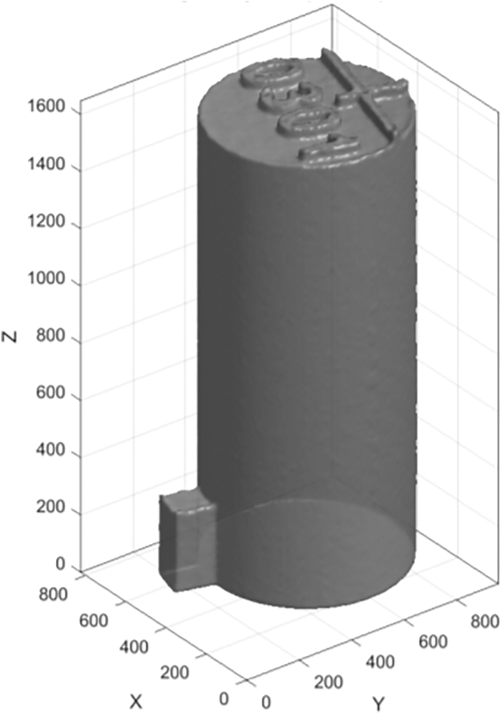
The proposed algorithm for ADR was formally evaluated using a test build for an MV-22B Osprey link from Merdes et al.²⁷ and Simpson,²⁸ shown on the left side in Figure 10. Experimental validation was carried out in MATLAB for pores only, that is, all $r_{-}$ data points. Although superdensities were present in the CT scan, they are generally rare, and the low numbers prevented us from performing rigorous validation. In addition, manual evaluation of resulting anomaly clusters pertaining to superdensities may prove difficult and erroneous. The CT scans were acquired at a resolution of 47 μm, yielding a CT image stack of dimension 588 × 3473 × 929, or 1.9 billion voxels, equivalent to 7.6 GB of memory at a single-precision resolution. ADR was carried out using a saliency threshold of $σ_{T} = 6$ and a mask erosion of $D^{\infty} (r) = - 470 μ m$ (or 10 voxels).

FIG. 10.

Left: Test coupon (NAVAIR Link) used to validate the ADR algorithm. Right: All 304 detected anomaly clusters.

Again, the latter prevents erroneous detections along the edge of the part that experiences significantly larger intensity gradients. The mask then contains 509 million voxels, roughly 27% of the entire X-ray CT image stack volume.

Kernel sizes of $n = 5, 7, 9, 11$ , corresponding to 235, 329, 423, and 517 μm, are used. Resulting anomaly voxels are subsequently consolidated over all the kernel sizes. Note that based on how the kernels are constructed in Equation (7), flagged defects are generally a lot smaller than the physical dimensions of the kernel. The ADR software then extracted 25,750 unique anomalous voxels, $r_{-}$ , satisfying both conditions: (1) $T_{n} (r_{-}) < μ_{n} - σ_{T} σ_{n}$ pores and (2) $T_{n} (r_{-}) = n^{3}$ (valid data points inside mask). All anomalous voxels, regardless of which kernel size was used to identify them, were subsequently combined into 304 clusters (or defects). The location of all clusters with respect to the part geometry is shown on the right side in Figure 10. Manual inspection of all the 304 clusters identified 30 FPs. Time to execute was about 2 min using a Dell Workstation at 3.5 GHz and an NVIDIA Tesla C2070 GPU with 6 GB memory.

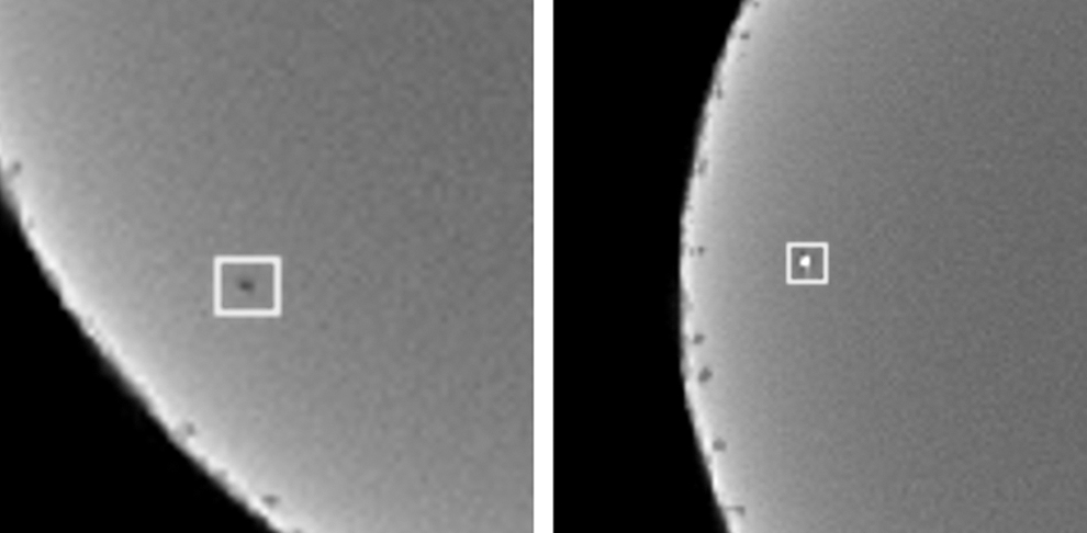
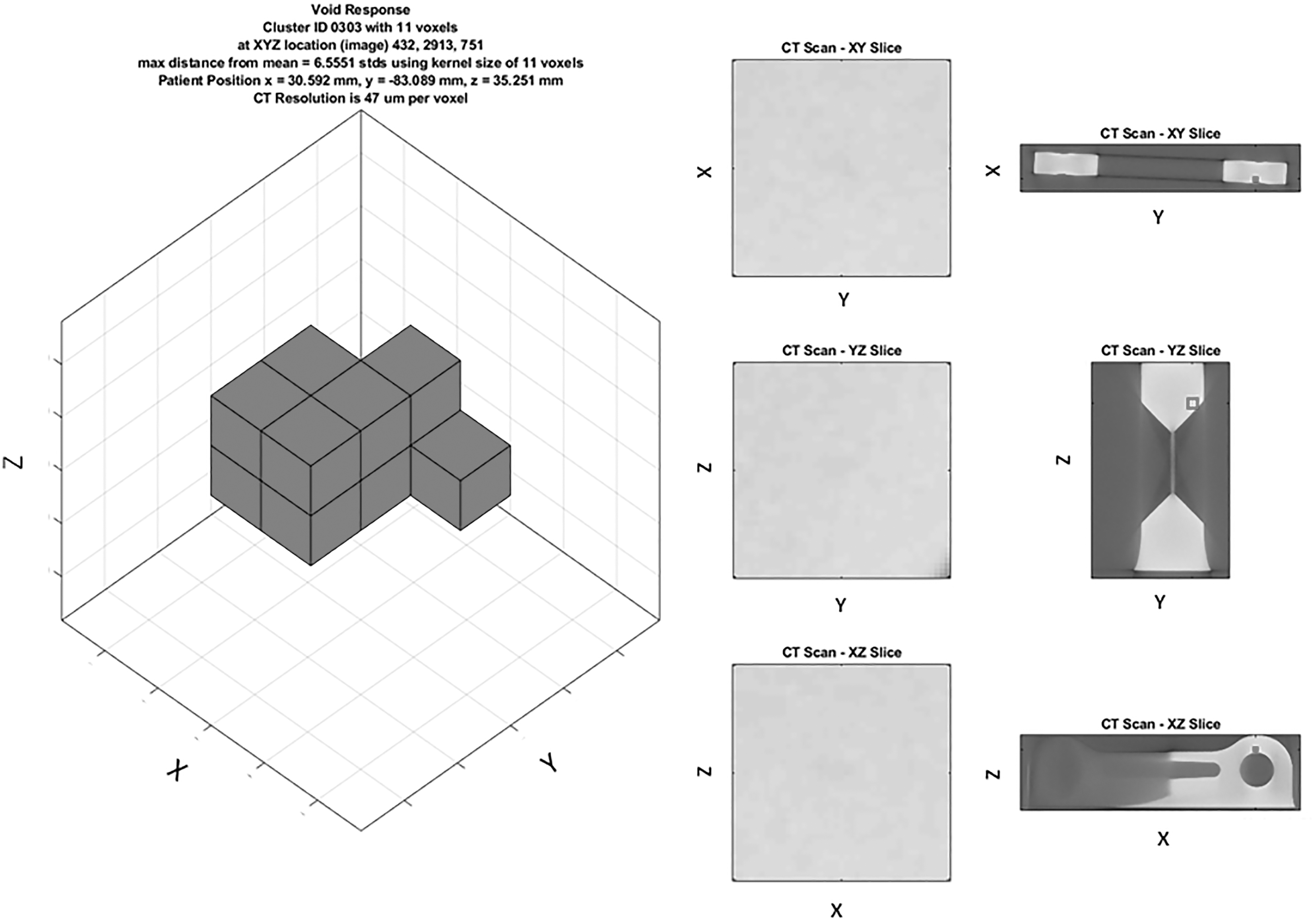
Figure 11 shows the most salient defect detected, here $σ = 37.8$ standard deviations from the mean. The ADR software provides a 3D view of the cluster on the left as well as 2D CT scan slices in the XY, XZ, and YZ planes. Those slices illustrate the intensity change (or saliency) of the defect relative to its local neighborhood. In addition, the software shows the actual defect location $r \in ℛ^{3}$ with respect to the part geometry. These plots are easily reconfigurable, and they are designed to present a quick overview of the most meaningful characteristics of the detected flaw.

FIG. 11.

Most salient defects detected with saliency $σ = 37.8$ . The defect consists of 399 voxels and thus has an equivalent diameter of 430 μm.

Similar to Figure 11, Figure 12 shows a defect that was labeled as an FP during manual inspection. At $σ = 6.5$ , this defect lacks saliency and is barely visible to the human eye in the CT slices. Again, Figure 12 illustrates the importance of the saliency threshold $σ_{T}$ from Equation (12) as a critical ADR parameter. Decreasing the saliency threshold will yield more detections but also increases the number of FPs within those detections. Similarly, increasing the saliency threshold will reduce the number of detections including the number of FPs, while increasing the risk of missed detections, that is, FNs.

FIG. 12.

Defect labeled as FP after manual inspection due to lack of saliency. FP, false positive.

Performance metrics for classification and detection algorithms are commonly derived using a fully populated confusion matrix,²⁹ including resulting numbers for TPs, FPs, FNs, and true negatives (TNs). In this application, the number of negative samples, that is, voxels that are not anomalous, outweighs the number of anomalous voxels by a factor of 20,000, making it a severely unbalanced classification problem. In addition, ground-truth data that label every single voxel as “defect” and “no defect” and the corresponding XYZ location within the entire CT scan of 509 million voxels is hard if not impossible to obtain.

For these reasons, we restrict our performance analysis to TPs, FPs, and FNs only. In other words, we select $σ_{T} = 6$ and the resulting 304 anomaly clusters including 30 FPs as a baseline for performance evaluation. This, in turn, assumes that the FN rate at $σ_{T} = 6$ is zero. Manual interrogation of each of the individual voxels to verify that assumption is clearly not possible.

When increasing the saliency threshold $σ_{T}$ , the classification output will change, and we can now determine the following:

TPs, number of remaining true detects,

FPs, number of remaining false detects, and

FNs, number of missed detections compared with the performance baseline with $σ_{T} = 6$ .

Figure 13 shows the progression of number of TPs, number of FPs, and number of FNs with increasing saliency threshold $σ_{T}$ . At $σ_{T} = 6$ , the ADR algorithm detects 304 anomalies with 274 TPs, 30 FPs, and 0 FNs. As $σ_{T}$ increases, the number of FPs reduces. At $σ_{T} = 8$ , all detected defects are TPs. While reducing the number of TPs, missed detections or the number of FNs increases. Those missed detections are the defects initially extracted and verified as true defects at $σ_{T} = 6$ . Figure 13 again shows the trade-off between FPs and FNs, which exists for any binary classification problem.

FIG. 13.

Progression of detection performance measured by number of TPs, number of FPs, and number of FNs as function of increasing saliency threshold parameter $σ_{T}$ . FNs, false negatives; TPs, true positives.

Using TPs, FPs, and FNs only, the following performance metrics for binary classification²⁸ can be derived. $\begin{matrix} P r e c i s i o n = \frac{T P s}{T P s + F P s} R e c a l l = \frac{T P s}{T P s + F N s} \\ F D R = 1 - P r e c i s i o n M R = 1 - R e c a l l \end{matrix}$ (13)

Here, FDR and MR represent the false discovery rate and miss rate, respectively. In addition, the F1-score, the geometric mean between recall and precision, is defined as $F 1 S c o r e = 2 \frac{P r e c i s i o n \times R e c a l l}{P r e c i s i o n + R e c a l l} = \frac{2 T P s}{2 T P s + F P s + F N s}$ (14)

Figure 14 shows the ADR performance as measured by the performance metrics outlined in Equations (13) and (14). Similar to Figure 13, those metrics are plotted as function of the saliency threshold $σ_{T} .$

FIG. 14.

Detection performance measured by precision, recall, and F1-Score (left) and FDR and MR (Right) as function of saliency threshold $σ_{T}$ . FDR, false discovery rate; MR, miss rate.

Again, one finds an increase/decrease in precision/recall with increasing $σ_{T}$ . Similarly, one sees a drop/rise in FDR/MR, respectively, when increasing $σ_{T}$ . Based on the results shown in Figures 13 and 14, one may find a reasonable trade-off between precision and recall, or similarly between the FDR and MR, at around $σ_{T} = 6.25$ . However, based on underlying requirements, the ADR algorithm may be tuned to achieve (1) a low MR with a higher FDR, or (2) a low FDR with a higher MR. Such a trade-off between Type I and Type II classification errors is inherent to any classification problem. For the application at hand, the trade-off may be governed by porosity requirements imposed by part certification guidelines. For example, the NDE guidelines define a maximum flaw size (such as MIL-STD-2219A—Fusion Welding for Aerospace Applications), which specifies a max surface porosity size of 0.030 inch (762 micron).

Conclusion

This article presents and validates a complete solution for automated anomaly detection in 3D CT scans that attempts to emulate visual cues used by human observers when detecting flaws. The algorithm is agnostic to part geometry and thus does not require additional input information such as CAD files. Initially, all voxels are categorized as “material” or “background” based on the underlying intensity statistics. All identified “material” voxels then determine the geometric shape of the part including the part surface. Defect detection is based on visual saliency of individual CT voxels, extracted using 3D convolution operations with separable kernels. Kernel separation allows for parallel and thus computationally efficient execution of the algorithm, enabling hardware acceleration using GPUs.

Design parameters include (1) the number and size of convolution kernels to be used, as well as (2) the actual threshold for saliency, that is, the convolution response, measured in standard deviations from the mean. All anomalous voxels are subsequently merged to form anomaly clusters that provide vital flaw information such as size, volume, orientation, and overall morphology. Overall computational complexity is manageable even for CT scans containing billions of voxels because all convolution operations are taking advantage of kernel separability and thus can be carried out in parallel.

Experimental results indicate that the proposed ADR algorithm performs well, with recall, precision, and F1 score well above 90%. Inherent trade-offs exist when specifying the saliency threshold for defect detection, which is generally the case for any binary classification problem. Decreasing the saliency threshold will yield more detected defects but also increase the FP rate. Increasing the saliency threshold will reduce the number of detected defects including the number of FPs. However, the number of missed defects, that is, FNs, will increase.

Future Work

Future work will include additional vetting of the ADR algorithms including a formal correlation between ADR performance and defect size and morphology. It is conceivable to predefine a minimum size for defects of interest, which would be aligned to standard practice in weld inspection that defines a maximum allowable flaw size. Currently, the majority of FPs or missed detections are caused by small defects, which generally have a lesser impact on part performance. In addition, computational complexity can be reduced when focusing only on defects of a certain size.

Although complete performance metrics including accuracy, which requires numbers for TNs, are difficult if not impossible to obtain, additional steps can be taken to provide ground truth using different detection techniques. Serial sectioning, for example, may be utilized to provide a rigorous comparison between actual defects and detected defects using just a subset of the data, that is, 2D slices.

One of the remaining limitations of the proposed algorithm is to detect defects at the edge of the part, which has been observed to be somewhat common in AM parts. Visual saliency is driven by the local CT intensity gradient, which is the largest between part and background, right at the edge of the part. Therefore, future work will focus on modifying the computation of visual saliency in those areas. It is conceivable to compute intensity gradients along the surface while filtering the components normal to it.

Footnotes

Acknowledgments

The authors would like to thank the Naval Air Systems Command and Penn State's Applied Research Laboratory for supporting this project. They also thank Mr. Zack Snow, Mr. Brett Diehl, Dr. David Corbin, and Mr. Griffin Jones for their technical feedback and their efforts in designing the experiments and in data acquisition.

Disclaimer

Any opinions, findings and conclusions, or recommendations expressed in this material are those of the authors and do not necessarily reflect the views of the Naval Air Systems Command (NAVAIR).

Author Disclosure Statement

No competing financial interests exist.

Funding Information

This material is based upon work supported by the Naval Air Systems Command (NAVAIR) under Contract No. N00024-12-D-6404, Delivery Order 0321.

References

Sames

, List

, Pannala

, et al. The metallurgy and processing science of metal additive manufacturing. Int Mater Rev, 2016; 61:315–360.

Gong

, Rafi

, Gu

, et al. Analysis of defect generation in Ti-6Al-4V parts made using powder bed fusion additive manufacturing processes. Addit Manuf, 2014; 4:87–98.

Yavari

, Ahmadi

, Wauthle

, et al. Relationship between unit cell type and porosity and the fatigue behavior of selective laser melted meta-biomaterials. J Mech Behav Biomed Mater, 2015; 43:91–100.

Liu

, Elambasseril

, Sun

, et al. The effect of manufacturing defects on the fatigue behavior of Ti-6Al-4V specimens fabricated using selective laser melting. Adv Mater Res, 2014; 891–892:1519–1524.

Spierings

, Schneider

. Comparison of density measurement techniques for additive manufacturing metallic parts. Rapid Prototyp J, 2015; 17:380–386.

Wits

, Carmignato

, Zanini

, et al. Porosity testing methods for the quality assessment of selective laser melted parts. CIRP Ann Manuf Technol, 2016; 65: 201–204.

Gegner

2D-3D conversion of object size distributions in quantitative metallography. In: Proceedings of the MMT-2006 Conference, Ariel, Israel, 2006.

Anton du

Plessis

, Igor

Yadroitsev

, Ina

Yadroitsava

, and Stephan

. Le Roux. 3D Printing and Additive Manufacturing. 2018; pp. 227–247. http://doi.org/10.1089/3dp.2018.0060.

Baniukiewicz

Automated defect recognition and identification in digital radiography. J Nondestr Eval, 2014; 33:327–334.

10.

Hou

, Wei

, Guo

, et al. Automatic detection of welding defects using deep neural network. J Phys Conf Series, 2017; 933. https://iopscience.iop.org/article/10.1088/1742-6596/933/1/012006

11.

Mery

, Arteta

. Automatic defect recognition in

X-ray testing using computer vision

. In: 2017 IEEE Winter Conference on Applications of Computer Vision (WACV). Santa Rosa, CA, 2017; pp. 1026–1035.

12.

Itti

Laurent

, and Christof

Koch

. “Learning to detect salient objects in natural scenes using visual attention. ” Image Understanding

Workshop

. 1999.

13.

Faiza

, Nacereddine

. Multiclass classification of weld defects in radiographic images based on support vector machines. In: 2014 Tenth International Conference on Signal-Image Technology and Internet-Based Systems. Marrakech, Morocco, 2014.

14.

Lawson

, Parker

Intelligent segmentation of industrial radiographic images using neural networks. In: Proceedings of SPIE. Boston, MA, United States: The International Society for Optical Engineering, 1994.

15.

Park

, Chung

, Seo

. Computed tomographic beam-hardening artefacts: Mathematical characterization and analysis. Philos Trans A Math Phys Eng Sci, 2015; 373.

16.

Jayaraman

TV.

Principles of radiography. In: ASM Handbook, Volume 17: Nondestructive Evaluation of Materials. Materials Park: ASM International 2018; pp. 383–409.

17.

ASTM International. E1441-19, Standard Guide for Computed Tomography (CT). West Conshohocken: ASTM International, 2019.

18.

Abella

, Martinez

, Desco

, et al. Simplified statistical image reconstruction for X-ray CT with beam-hardening artifact compensation. IEEE Trans Med Imaging, 2020; 39:111–118.

19.

McLachlan

, Peel

Finite Mixture Models. Hoboken, NJ: John Wiley & Sons, Inc., 2000.

20.

Shapiro

, Stockman

. Computer vision. The University of California, Los Angeles, CA: Prentice Hall, 2001; pp. 137–150.

21.

Maurer

, Rensheng

, Raghavan

. A linear time algorithm for computing exact euclidean distance transforms of binary images in arbitrary dimensions. IEEE Trans Pattern Anal Mach Intell, 2003; 25:265–270.

22.

Morgan

, Morgan

, Natale

, et al. Selection and installation of high resolution imaging to monitor the PBFAM process, and synchronization to post-build 3D computed tomography. In: 29th Annual International Solid Freeform Fabrication Symposium, Austin, TX,. 2017.

23.

Niebur

, Kock

, Itti

. A model of saliency-based visual attention for rapid scene analysis. IEEE Trans Pattern Anal Mach Intell, 1998; 20:1254–1259.

24.

Cong

, Lei

, Fu

, et al. Review of visual saliency detection with comprehensive information. IEEE Trans Circuits Syst Video Technol, 2018; 29:2941–2959.

25.

Gobert

, Reutzel

, Petrich

, et al. Application of supervised machine learning for defect detection during metallic powder bed fusion additive manufacturing using high resolution imaging. Addit Manuf J, 2018; 21:517–528.

26.

Mathworks Inc., Find connected components in binary images via bwconncomp, MATLAB documentation, 2020.

27.

Merdes

, Reutzel

, Mitchell

, et al. Additively Manufactured MV-22B Osprey Flight Critical Components: Production Data for Witness Coupons and Test Specimens, Pennsylvania State University Applied Research Laboratory, State College, PA, Technical Report,. 2020.

28.

Simpson

. “Are AM Parts as

Strong?

, ” Modern Machine

Shop

, 2017. https://www.mmsonline.com/columns/are-am-parts-as-strong (last accessed June 7, 2022).

29.

Fawcett

An Introduction into ROC Analysis. Pattern Recogn Lett, 2006; 27:861–874.