Anomaly Detection in Fused Filament Fabrication Using Machine Learning

Abstract

Fused filament fabrication (FFF) has been widely used in various industries, and the adoption of technology is growing significantly. However, the FFF process has several disadvantages like inconsistent part quality and print repeatability. The occurrence of manufacturing-induced defects often leads to these shortcomings. This study aims to develop and implement an on-site monitoring system, which consists of a camera attached to the print head and the laptop that processes the video feed, for the extrusion-based 3D printers incorporating computer vision and object detection models to detect defects and make corrections in real-time. Image data from two classes of defects were collected to train the model. Various YOLO architectures were evaluated to study the ability to detect and classify printing anomalies such as under-extrusion and over-extrusion. Four of the trained models, YOLOv3 and YOLOv4 with “Tiny” variation, achieved a mean average precision score of >80% using the AP50 metric. Subsequently, two of the models (YOLOv3-Tiny 100 and 300 epochs) were optimized using Open Neural Network Exchange (ONNX) model conversion and ONNX Runtime to improve the inference speed. A classification accuracy rate of 89.8% and an inference speed of 70 frames per second were obtained. Before implementing the on-site monitoring system, a correction algorithm was developed to perform simple corrective actions based on defect classification. The G-codes of the corrective actions were sent to the printers during the printing process. This implementation successfully demonstrated real-time monitoring and autonomous correction during the FFF 3D printing process. This implementation will pave the way for an on-site monitoring and correction system through closed-loop feedback from other additive manufacturing (AM) processes.

Introduction

Fused filament fabrication (FFF) is an extrusion-based additive manufacturing (AM) process commonly used to fabricate polymeric¹ and composites parts.^2–4 It has also been used to fabricate metal parts⁵ with a few additional postprocessing steps. Owing to the wide variety of available materials and the mature printing operations, many industries such as aerospace,⁶ biomedical,⁷ pharmaceutical,^8,9 automotive,¹⁰ and sports¹¹ industries have adopted FFF. It is also the most well-established AM process with lower material wastage, making it more environmental friendly.¹²

Despite its ability to create complex geometries and customizable functional parts, FFF is not completely free from errors in the printing process. Three-dimensional printing defects alter the mechanical properties of 3D printed parts. Changes in properties often lead to poor mechanical strength or even poor surface finish,¹³ which often requires postprocessing techniques such as thermal aging¹⁴ to improve the mechanical properties.

In addition, defective printed parts often lead to wasted material. Typical defects include over-extruded and under-extruded filament. Over-extrusion occurs when too much material is extruded onto the layer. Over-extruded layers are often caused by a high filament feed rate. This causes the material to “overflow,” resulting in small beads on the edges and uneven surfaces of the object. On the contrary, under-extrusion occurs when the 3D printer does not extrude sufficient material onto the layers. Under-extruded layers are caused by a low filament feed rate, leading to gaps in between the adjacent layers.¹⁵ Ultimately, this results in the component having poor mechanical properties. These defects are often caused by the lack of monitoring technique to check the amount of material extruded.

Efforts have been made to minimize or eliminate defects in 3D printing by optimizing print settings, design compensation, and postprocessing. However, these methods are based on trial and error or require complex modeling to compensate for any form of defect that might alter the shape or size of the 3D printed component.¹⁶ This, therefore, emphasizes the importance of early fault detection so that on-site repairs can be carried out. This is where in situ monitoring of FFF comes into the picture.

There are several implementations of in situ monitoring systems in FFF 3D printers. For example, various sensors such as acoustic emission (AE) sensors,¹⁷ vibration sensors,¹⁸ temperature-based sensors,¹⁹ and optical methods²⁰ are used to acquire data from the fabrication processes.

Typically, condition indicators (Cis) were used to detect fault in the printing process. For example, Yoon et al. implemented a fault diagnosis and monitoring system using a condition monitoring algorithm to detect faults in the machine state that produced lower print quality.²¹ Yoon et al. successfully detected the induced fault after validating the performance of each Cis. The use of the condition monitoring method offers advantages, such as the flexibility of using different types of sensors and the use of a variety of Cis to improve the detection system. However, a proper selection of the Cis has to be carried out to ensure accurate detection of anomalies to avoid false interpretations.

The multiparameter complexity and the need for quality control in 3D printing (including monitoring) have turned researchers to machine learning.^22–25 Machine learning models, such as the convolutional neural network (CNN) models detect important features on their own without human supervision. The ability of the machine learning algorithms to learn to detect and classify anomalies from the large dataset of signals and images eliminates the need to identify suitable Cis.²⁶ Although some studies are devoted to the classification and detection of abnormalities or defects, most of them lead to binary classification, namely “defective” and “non-defective” or “normal” and “abnormal.”

In addition, the research mentioned previously often lacks the ability to correct and refine print defects in the on-site monitoring system. For instance, Jin et al. trained various types of CNN models to classify under-extrusion and over-extrusion of layers during the FFF 3D printing process. By doing so, a 98% classification accuracy score was yielded for the defects detection.²⁰ During the monitoring phase, images were captured over a specified interval and were then fed into a classification model. The defects detected would then be remedied through the self-correction process. However, the correction process takes place only on subsequent layers. Thus, the defects present on the previous layers could not be corrected. Therefore, there is a lack of research on the ability to identify and mark specific defects and then correct them on the spot.

Object detection deep learning models, on the contrary, can detect multiple objects and identify their locations within the image. Some common object detection models, such as ResNet²⁷ and YOLO,²⁸ have been used to help improve the manufacturing workflow. For instance, YOLO has been used to quickly detect capacitors with an average detection time of <0.3 s for the printed circuit board (PCB) optical inspection.²⁹ YOLOv3 has been used to detect part defects of darning needles, such as crocked shapes, length size errors, wringing errors, and endpoint size errors with an accuracy rate of 92.8%.³⁰ The use of the object detection models generally focused on the inspection of the parts after they are manufactured.

For an independent inspection system equipped with a self-calibration function, the system needs to know the specific types of defects to make appropriate corrections. The objective of this study was to study the effectiveness of the object detection model to detect printing defects such as over-extrusion and under-extrusion for closed-loop feedback control. Previous research achieved a frame rate of 20 frames per second (FPS),²⁰ which is lower than the usual frame rate (30 FPS) of cameras. Our study puts emphasis on improving the inference speed and thus the frame rate. The focus of this study was mainly the detection phase in the in situ monitoring system and the self-correction of the printing process through G-code modification.

In particular, various YOLO models were evaluated to identify, classify, and mark defects accordingly. Model optimization was performed by converting to Open Neural Network Exchange (ONNX) format for the deployment of the object detection model in the monitoring system to further improve the inference speed. Owing to the lack of relevant training data, a dataset containing various printing conditions was created to train the object detection models. A self-corrective algorithm was also proposed to perform corrective printing.

Experimental Methodology

The in situ monitoring and correction system for an FFF 3D printer consisted of three segments: real-time monitoring, defects detection, and print correction as given in Figure 1. In the first segment, the camera captured images from a 3D printing process. The captured image data were then fed into a trained object detection model, which is the second segment. Finally, the classification from the object detection model determined the actions to be taken to perform corrections if there were defects present (third segment).

FIG. 1.

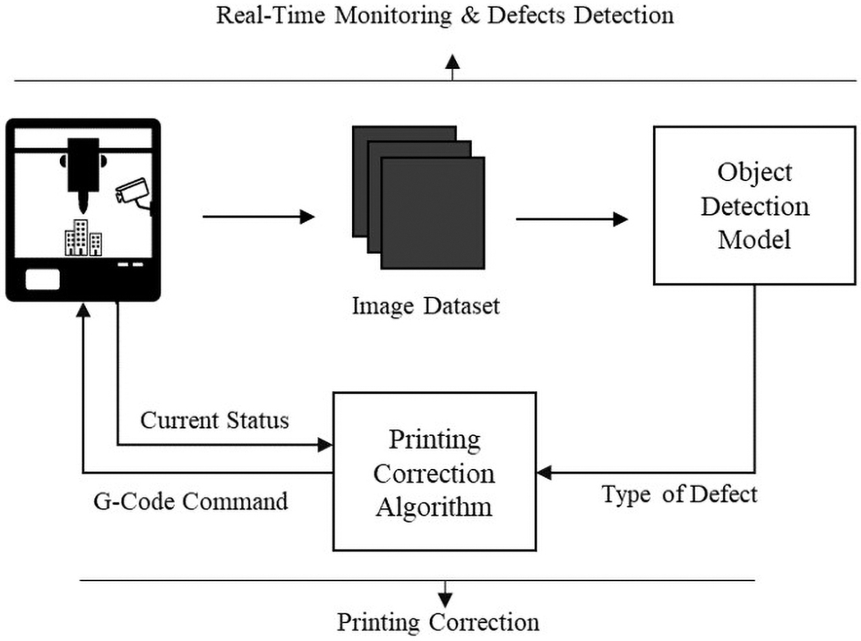
An illustration of the full in situ monitoring and self-correction system.

To develop an in situ monitoring and correction system for an FFF 3D printer, there are three phases: acquire image data, train object detection model, and develop correction algorithm. Each phase is described in detail in the following subsections and self-correction system.

Training data acquisition

To train the object detection model, an image dataset that showed the various defects is required for training. For this project, a dataset that consisted of three defects classes (normal, over-extrusion, under-extrusion) was generated, as there are no available sources to obtain the FFF-related defects dataset. The training dataset was generated manually.

The proposed method to acquire image data was through a camera. The Logitech C310 HD Webcam was selected to capture the images during the 3D printing process. The Logitech C310 HD Webcam was attached to the EasyArts Ares FFF 3D Printer's extruder hot end as given in Figure 2. The Logitech C310 HD Webcam captured images from the 3D printer's printing process at ∼3 s intervals.

FIG. 2.

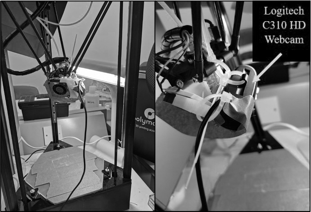
Experimental setup for training data acquisition using a makeshift attachment to mount the Logitech C310 HD Webcam on EasyArts Ares' hotend.

A few basic image processing steps were performed using the OpenCV library before exporting them into image data. The basic image processing techniques included converting the captured images into grayscale images and segmenting the images into smaller images so that these images could be processed rapidly in the later phases. The images captured were then filtered manually to remove noises so that the training accuracy during the object detection would not be affected.

Polylactic acid filament was used on the EasyArts Ares FFF 3D printer to print sample defective and nondefective parts. To obtain the images of various printing conditions, the printing parameters such as printing speed and flow rate were modified to introduce instability to the printing process. In addition, the printing speed was significantly reduced to allow clear image capture. For each type of defect, a 50 mm diameter × 5 mm thickness 3D model was printed. The images were classified into three groups, that is, normal, under-extrusion, and over-extrusion. A total of 18,000 images were collected, in which 8000 images were classified as normal, 5000 images were classified as over-extrusion and under-extrusion each. The image data collected were then utilized to train the object detection model. Samples of the obtained image data are given in Figure 3.

FIG. 3.

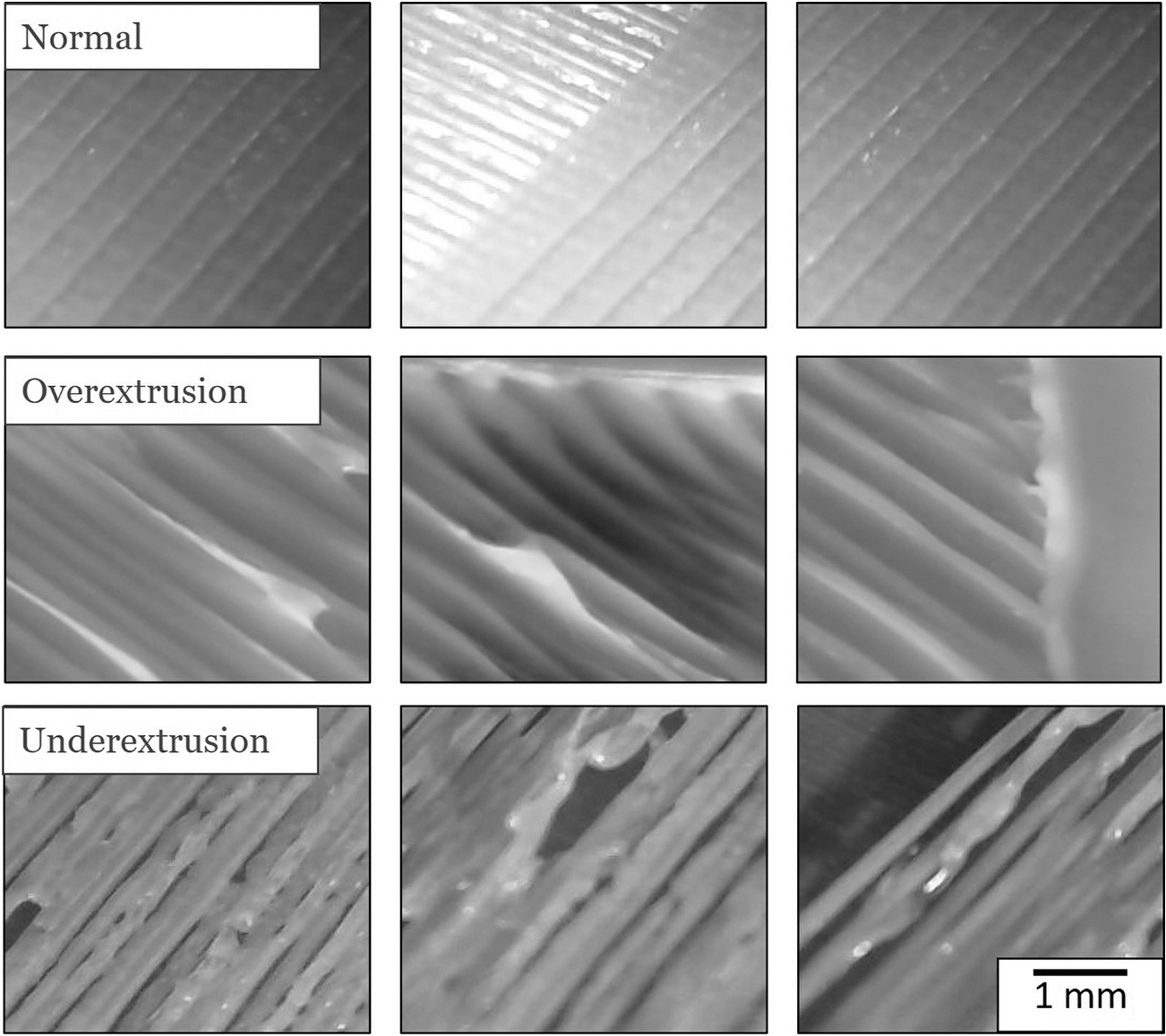
Sample image data of the Normal, Over-extrusion and Under-extrusion classes.

Object detection model

Three object detection models were selected in this study to learn to classify the images. The models were YOLOv3, YOLOv3-Tiny, and YOLOv4-Tiny.

The YOLOv3 model used Darknet-53 CNN architecture as given in Figure 4. A variation of the YOLOv3 model, YOLOv3-Tiny, uses a simplified architecture from the parent model.³¹ The “tiny” version of the model boasts a faster inference speed but with lower accuracy. Both these models would be trained and validated with the generated dataset to determine if the models were suitable for the in situ monitoring system. In addition, a newer version of the model, YOLOv4, which has faster inference speed and higher accuracy³² would also be trained and validated. However, owing to hardware limitations, only the “tiny” version of the YOLOv4 model would be trained.

FIG. 4.

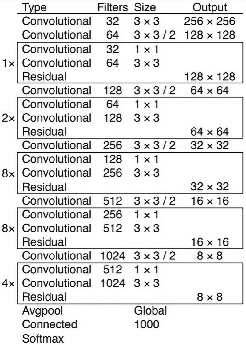
Backbone of the YOLOv3 model, Darknet-53 architecture, adapted from YOLOv3.³¹

A summary of the models' architectures is given in Table 1. The YOLOv3 and the YOLOv4-Tiny use a variant of an activation function called Rectified Linear Unit (ReLU). The ReLU activation function applies the nonlinear transformation to the data. The advantages of using the ReLU activation function were fast computation and the activation function does not suffer from vanishing gradients. This makes the YOLO models fast and accurate for classifications.

Table 1.

Summary of the Models' Architectures with the Respective Number of Layers and Activation Functions Adapted From Refs.^31,32

Model	Model architecture size			Activation function
Model	No. of convolutional layers	No. of other layers (shortcut/route/upsample/pooling, etc.)	Total	Activation function
YOLOv3	75	31	106	Leaky ReLU
YOLOv3-Tiny	16	5	21	Leaky ReLU
YOLOv4-Tiny	21	17	38	Leaky ReLU

ReLU, Rectified Linear Unit.

Self-correction of 3D printing defects

Self-correction for this application performs corrective actions on the 3D printing process through G-code commands.

The self-correction algorithm uses a Python library, Selenium, which is an open-source web-based automation tool. As the 3D printer's OctoPrint interface is browser-based, an algorithm could be used to “hook” onto the browser interface to read and send G-code commands. It should be noted that the EasyArts Ares 3D printer uses RepRap as the G-code “flavor.” Thus, the commands used are based on RepRap G-codes.

The self-correction algorithm generates corrective actions based on the defect classification given by the trained object detection model. As the classification takes place at a rapid rate (e.g., 60 classifications in 1 s) during the printing process, the classified class confidence is averaged to accurately determine the defects present.

In this study, a self-correction algorithm was designed to perform simple corrections for two types of 3D printing defects: under-extrusion and over-extrusion. The defects were introduced during the printing process by changing the printing parameters. The self-correction algorithm reads the executed G-code commands from the 3D printer's browser-based console and stores the last five commands. If defects were present, the algorithm would output and execute G-code commands to perform correction through the console automatically.

A simplified illustration of how the self-correction algorithm functions are given in Figure 5. The algorithm takes the classification result and the confidence level from the object detection model. If a defect was detected, the classifications would be either the over-extrusion class or the under-extrusion class. Otherwise, the algorithm continues to obtain the classifications if no defects were detected. If a defect was present, a Python Dictionary would count the occurrence of the defect and sum the confidence level. Then, an average was taken based on the sum of the confidence level against the number of occurrences. This prevents the correction algorithm from being “reactive” by performing correction immediately when a defect occurs. The algorithm then checks the average confidence and the count against the specified threshold before the correction for a particular defect could take place.

FIG. 5.

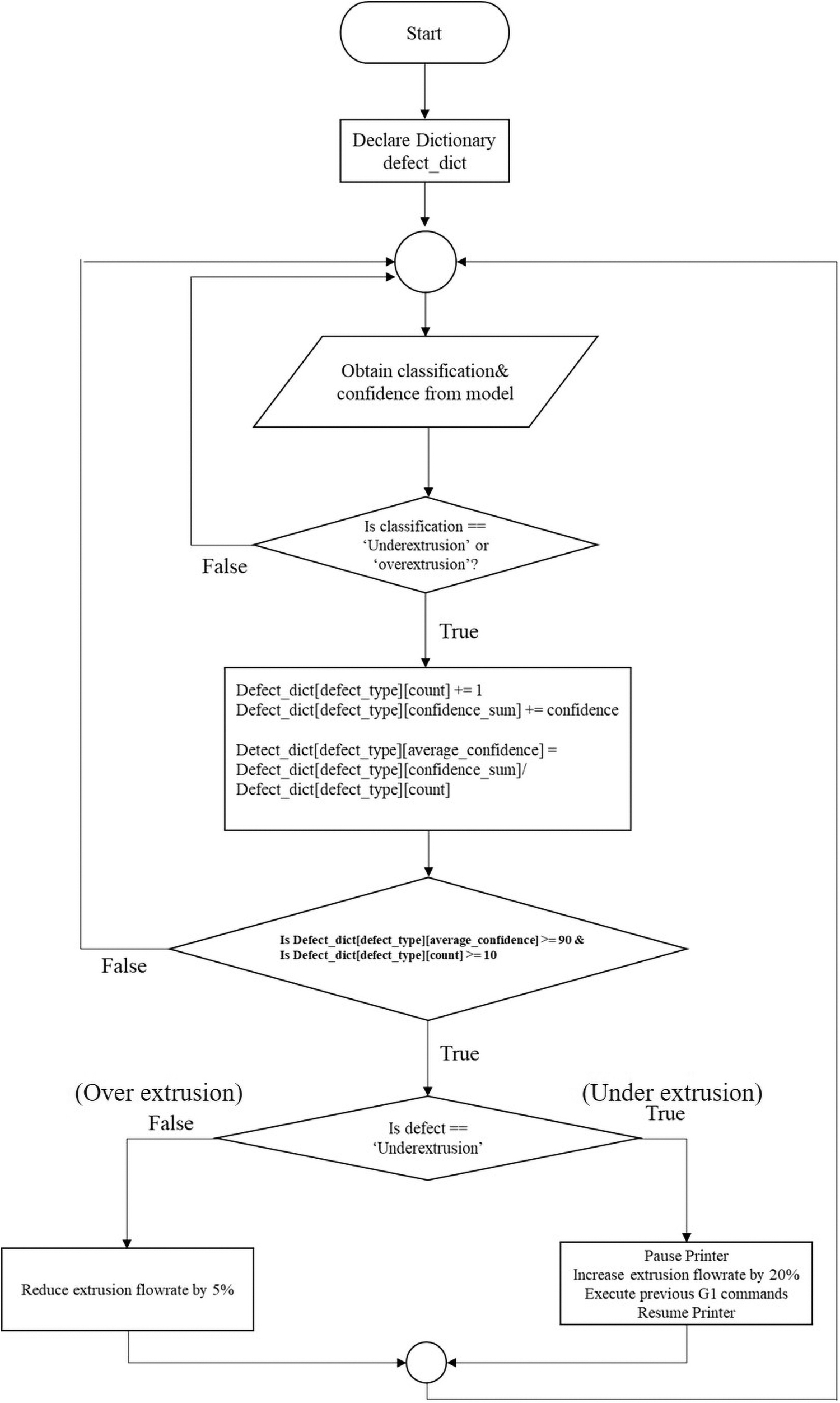
Simplified flowchart of the self-correction algorithm.

The corrective actions of the chosen defects for the self-correction algorithm are proposed and summarized in Table 2.

Table 2.

Summary of the Proposed Corrective Actions for the Respective Three-Dimensional Printing Defects

Defect type	Corrective action
Under-extrusion	1. Increase the material flow rate 2. Reprint the affected areas by re-running the last few G-code commands
Over-extrusion	1. Decrease the material flow rate

Results and Discussion

Table 3 summarizes the evaluation for both the training and performance of the models. The average precision (AP) and mean average precision (mAP) scores computed are based on the AP50 metric. The AP50 metric is selected because it is sufficient to evaluate the performance of the trained model. In addition, the metric allows direct comparison with other object detection models. On the contrary, the AP75 metric provides a stricter evaluation of the trained models. However, the AP75 metric will not be used in this project as sample evaluations of the models showed insignificant changes in the scores. The hardware used for evaluating the inference speed is given in Table 4.

Table 3.

Summary of Validation Losses, Average Precision Scores, and Inference Speed for All Models Trained

Model		Validation loss			Computed AP score and mAP score, %				Inference speed, FPS
Type	Epochs	Confidence	IoU	Total	Normal class	Over-extrusion class	Under-extrusion class	mAP	Inference speed, FPS
YOLOv3	48	6.768 × 10⁻⁴	9.778 × 10⁻³	0.3137	98.247	96.941	29.083	74.757	4.46
YOLOv3	100	1.056 × 10⁻⁵	15.400 × 10⁻³	0.4989	89.559	79.195	97.981	88.912	4.56
YOLOv3-T	100	1.106 × 10⁻⁵	15.300 × 10⁻³	0.5442	91.158	81.049	97.303	89.837	18.00
YOLOv3-T	300	1.908 × 10⁻⁶	12.540 × 10⁻³	2.1030	91.156	81.048	97.303	89.836	16.90
YOLOv4-T	100	8.817 × 10⁻⁶	15.610 × 10⁻³	0.6097	97.092	96.915	24.382	72.796	19.16
YOLOv4-T	500	1.344 × 10⁻⁶	11.500 × 10⁻³	1.7380	90.920	79.766	95.864	88.850	18.72

AP, average precision; FPS, frames per second; IoU, intersection over union; mAP, mean average precision.

Table 4.

Specifications of the Hardware Used During the Evaluation

Hardware type	Laptop
Memory size	8 GB RAM
CPU model	Intel Core i5-8250U @ 1.60 GHz (8 CPUs)
GPU model	Nvidia MX130

The confidence validation loss, the intersection over union (IoU) validation loss, and the total validation loss are given in Table 3. The confidence loss measures the objectness of a predicted bounding box. Lower confidence loss indicates higher objectness, or in other words, more likely an object exists within the predicted bounding box. The IoU is an evaluation metric that measures how close the predicted bounding box is to the ground truth. Lower IoU loss indicates that predicted bounding boxes have high overlapping percentages with the ground truths. The total validation loss combines both the confidence and IoU losses.

The total validation losses for each model are relatively low with some variations in the losses among the models. This means that the learning process for the models was effective for the given dataset. It is found that for YOLOv3-T the total validation loss is higher in 300 epochs compared with 100 epochs, suggesting overfitting of the model. The same pattern is observed for YOLOv4-T: the total validation loss is higher in 500 epochs compared with 100 epochs. It is also found that the larger YOLOv3 could achieve lower total validation loss compared with the tiny versions. Of all the trained tiny models, YOLOv3-T trained with 100 epochs gives the lowest validation loss.

Figure 6 provides the results of the AP and mAP scores with the respective inference speed for each model.

FIG. 6.

Graphs of (a) the AP and mAP scores of each class and (b) the inference speed for all the trained models. AP, average precision; mAP, mean average precision.

Variations on the scores and the inference speed could be seen across various models. The YOLOv3 (48 epochs) model has high AP scores for the normal and over-extrusion classes (98.247% and 96.941%, respectively). However, the AP score for the under-extrusion class (29.083%) is significantly lower, which reduces the mAP score. The low AP score for the under-extrusion class could be owing to the low number of epochs used for training. The YOLOv3 (100 epochs), however, scored better in the metrics with a higher AP score for the under-extrusion class (97.981%), which increased the mAP score. However, there were reductions in the AP scores for both the normal and over-extrusion classes (89.559% and 97.981%, respectively). Nevertheless, the increase in the number of epochs did improve the performance of the model (based on AP50 metrics).

The “Tiny” variant of the YOLOv3 models was trained with a higher number of epochs because the architecture is smaller than its parent model. With the smaller architecture size, the time required to train the model would be lesser compared with the parent model. The YOLOv3-Tiny (100 epochs) model scored high AP scores for the normal and under-extrusion classes (91.158% and 97.303%, respectively) with a lower AP score for the over-extrusion class (81.049%). Despite the increase in the number of epochs, the YOLOv3 (300 epochs) model did not have any significant improvement to the AP and mAP scores.

The YOLOv4 model uses an improved architecture that boasts better inference accuracy and inference speed. However, for this project, only the “Tiny” variant is trained. The YOLOv4-Tiny models were also trained at a higher number of epochs because of their architecture size. The YOLOv4-Tiny (100 epochs) model has high AP scores for the normal and over-extrusion classes (97.092% and 96.915%, respectively) but a low AP score for the under-extrusion class (24.382%). In addition, the scores are lower than the YOLOv3-Tiny (100 epochs) model. The YOLOv4-Tiny (500 epochs) model scored higher in the under-extrusion class (95.864%). However, there were reductions in the scores for the other two classes. This could mean that the model is being overfitted. Nonetheless, the increased number of epochs to 500 epochs improved the model's performance.

Through observation, the increase in the number of epochs tends to improve the models' mAP scores. However, not the same can be said for the inference speed. The inference speed of the model depends on the hardware used for implementation. For example, the trained YOLOv3 models' inference speeds are significantly lower (∼4.5 FPS) compared with the other models. This is owing to the large model size with greater number of layers that requires more computations. The “Tiny” variant of the model has its inference speed almost four times the parent model (16–18 FPS). This “Tiny” variant model requires lesser computations owing to the smaller model size. Similarly, the YOLOv4-Tiny models have higher FPS because of the small model size. A sample of the YOLOv3-Tiny (300 epochs) model used for real-time classification is given in Figure 7a and b.

FIG. 7.

A sample of a real-time defect classification. (a) Under-extrusion with 88% confidence. (b) Normal with 97% confidence using the YOLOv3-Tiny (300 epochs) model. A sample of a defect classification with a significant increase in FPS, (c) 92.8 FPS, and (d) 85.4 FPS using an optimized YOLOv3-Tiny (300 epochs) in ONNX Runtime. FPS, frames per second; ONNX, Open Neural Network Exchange.

For the models with high mAP scores, the inference speed ranges between 16.9 FPS and 18.72 FPS, which is significantly lower than the camera's frame rate of 30 FPS. This could lead to inaccuracies in the classification as lesser image data are captured during a certain interval. However, further optimization could be performed on the models to improve the inference speed. Although optimization of models could be performed to improve the inference speed, it would not be beneficial to optimize the models with significantly low inference speed such as the YOLOv3 (48 and 100 epochs) models because the other models have significantly higher inference speed with similar or better mAP scores.

To further improve the inference speed, the model optimization is performed to convert the trained model into ONNX format and use the ONNX Runtime, which is a performance-focused engine for ML models.³³ ONNX format is an open format for ML models that can be used in various ML tools and frameworks. The conversion to ONNX format optimizes the trained model by removing redundant nodes and fusing multiple nodes into a single node in the trained model's graph. These optimizations reduce the computations needed during classification. Then, the ONNX Runtime further accelerates the inference performance of the model.

An advantage of using the ONNX Runtime is that it significantly improves the inference performance of models that run on the CPU only. This means that the application does not require high-performing GPUs to run these models. The YOLOv3-Tiny (100 and 300 epochs) models were selected for optimization as they have the highest mAP scores. The results of the optimization of the selected models are given in Table 5. A sample of the optimized YOLOv3-Tiny (300 epochs) model being used in a 3D printing process is given in Figure 7c and d.

Table 5.

Summary of the Optimized Models' Inference Speed

Model	Original inference speed, FPS	Optimized inference speed (average), FPS
YOLOv3-Tiny, 100 Epochs	18	70
YOLOv3-Tiny, 300 Epochs	16.9	68

Table 5 shows a significant increase of almost four times for the inference speed of these models. Lower inference speed means that lower image acquisition rate has to be used and it greatly increases the chances of missing the defects. To compensate for the lower frame rate, the print speed has to be lowered. However, lowering the print speed lengthens the print time and it is not practical from the economy point of view. Therefore, higher frame rate is generally preferable because this means that more image data could be captured within a certain interval and the print speed can be higher.

This 68 FPS that the optimized model is capable of processing is higher than the image acquisition rate (30 FPS) of the camera. Thus, the optimized model would not cause a bottleneck that limits the real-time in situ correction ability and the optimized model gives room for future system upgrades. In contrast, if the original model were to be used, the image acquisition rate of the camera would have to be lowered.

The correction process was carried out autonomously when defects were detected. The corrective commands were successfully executed. However, the latency between the detection of defects and the execution of the correction commands was not consistent. One possible reason is that the printer has to complete its current command before pausing and would only execute the corrective commands when the nozzle completely stops. Subsequently, the corrective commands were then executed and the corrections took place with no issues. Figure 8 shows the comparison between the normal printing process and the printing process with print corrections for a sample 30 × 30 mm square part.

FIG. 8.

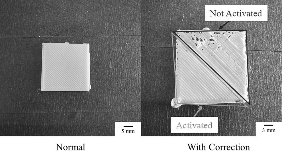
A comparison of a 30 × 30 mm print between normal print and under extruded print with not corrected and corrected prints.

From Figure 8, the print with corrections shows two different print qualities at two different regions. During the printing process, the printing parameters were modified to force the under-extrusion to occur. Initially, the corrective algorithm was not activated on purpose to show the difference before and after the correction. It can be seen that the extruded filaments were not continuous and pores were present. Once the correction algorithm was activated, the algorithm made the necessary correction by increasing the flow rate of the extruder once it detected that under-extrusion has occurred from the object detection model.

A comparison between the normal print and the print with corrections shows some differences in the quality of the prints. For example, the print with corrections shows gaps between the layer and the inner wall. In addition, there were some inconsistencies in the extrusion owing to the varying flow rate throughout the printing process. This shows that further optimization of the correction commands is required.

In summary, the implementation of the system demonstrates the autonomous classifications and corrections of the 3D printing process. The system could perform classifications with high accuracy and simple corrections. However, the implementation also exposes several limitations of the system that require further optimizations before the system could be used in actual 3D printing processes. This includes ensuring that the camera is properly focused to allow for proper detection of anomalies during the printing process.

Conclusion

The lack of good quality control in the 3D printed parts has led to the slow adoption of the additive manufacturing techniques in many industries. The use of on-site monitoring system is key to ensuring high-quality printed parts by having closed-loop feedback control. This project demonstrates the implementation of anomaly detection on a FFF 3D printer and has carried out the analysis and evaluation of the implementation. The implementation of the system involves several main components: sensor, classification model, and correction algorithm. In particular, the various YOLO architectures were evaluated to study the ability to detect and classify printing anomalies such as under-extrusion and over-extrusion. Based on the evaluations of the models, the results shown were promising in classifying the defects fast and accurately.

Four of the trained models, YOLOv3 and YOLOv4 with “Tiny” variation, achieved an mAP score of >80% using the AP50 metric. Subsequently, two of the models (YOLOv3-Tiny 100 and 300 epochs) were optimized using ONNX model conversion and ONNX Runtime to improve the inference speed. A simple correction algorithm was developed to perform corrective actions on the defects. The components, the sensor, the classification model, and the algorithm were put together to form the in situ monitoring system. The successful demonstration of the real-time printing correction can potentially cause a paradigm shift in the way how manufacturing is conducted. Having better quality control over the printed parts improves the productivity and cost-efficiency of the manufacturing line, thus, attracting more industry players to adopt the 3D printing techniques.

One of the limitations of this project is the lack of availability of image data of 3D printing defects. Thus, data collection of the image data had to be carried out in the early phase of the project that consumed a significant amount of time. In addition, the visual sensor used is limited to only 30 FPS. This means that the 3D printing process had to be significantly slowed down to allow the sensor to capture clear images. This significantly increased the printing time.

Future work could include having a more robust classification model, that is, more data have to be collected for training. For instance, the model has to learn to differentiate between defects and “designed porosity.” In addition, the data could include other forms of defects, such as weak infill, overheating, and curling, to improve the classification capabilities of the system to detect more types of 3D printing defects. With the larger dataset, hardware that has sufficient computational capabilities to process these data and use them for training would be critical to prevent significant time wastage.

In addition, the correction process could be improved if the latency between the console and the 3D printer is reduced. Perhaps, it would be better if the in situ monitoring system is implemented at a lower level of the 3D printer, that is, controller level. As the correction capabilities are currently limited, future projects could focus on improving the correction process to cover correction on other affected regions and to correct other types of defects.

Footnotes

Authors' Contributions

G.D.G.: Conceptualization, Writing—Original Draft, Resources.

N.M.B.H.: Data Curation, Formal analysis, Investigation, Writing—Original Draft.

W.Y.Y.: Resources, Writing—Review and Editing, Supervision.

Author Disclosure Statement

No competing financial interests exist.

Funding Information

This research is supported by the National Research Foundation, Prime Minister's Office, Singapore under its Medium-Sized Centre funding scheme.

References

Goh

, Yap

, Tan

, et al. Process–structure–properties in polymer additive manufacturing via material extrusion: A review. Crit Rev Solid State Mater Sci, 2020; 45:113–133.

Goh

, Yeong

, Mode

I interlaminar fracture toughness of additively manufactured carbon fibre thermoplastic

. In: Proceedings of the 3rd International Conference on Progress in Additive

Manufacturing

. Chua CK (Ed), Nanyang Technological

University

, Singapore. 2018; pp. 505–510.

Jiang

, Ning

. Fused filament fabrication of biodegradable PLA/316L composite scaffolds: Effects of metal particle content. Procedia Manuf, 2020; 48:755–762.

Yeong

, Goh

. 3D printing of carbon fiber composite: The future of composite industry?. Matter, 2020; 2:1361–1363.

Gong

, Snelling

, Kardel

, et al. Comparison of stainless steel 316L parts made by FDM-and SLM-based additive manufacturing processes. JOM, 2019; 71:880–885.

Joshi

, Sheikh

. 3D printing in aerospace and its long-term sustainability. Virtual Phys Prototyp, 2015; 10:175–185.

Luis

, Pan

, Sing

, et al. Silicone 3D printing: Process optimization, product biocompatibility, and reliability of silicone meniscus implants. 3D Print Addit Manuf, 2019; 6:319–332.

Wong

, Xu

, Kang

, et al. Development of a 3D-printed medication label for the blind and visually impaired. Int J Bioprinting, 2020; 6.

Bishop

, Leigh

. Using large-scale additive manufacturing as a bridge manufacturing process in response to shortages in personal protective equipment during the COVID-19 outbreak. Int J Bioprinting, 2020; 6:51–58.

10.

Nichols

MR.

How does the automotive industry benefit from 3D metal printing?. Met Powder Rep, 2019; 74:257–258.

11.

Soltani

, Noroozi

, Bodaghi

, et al. 3D printing on-water sports boards with bio-inspired core designs. Polymers, 2020; 12:250.

12.

Jiang

, Xu

, Stringer

A new support strategy for reducing waste in additive manufacturing. In: Xun Xu, Mohamed I. Dessouky, Ray Y. Zhong (Eds). The 48th international conference on computers and industrial engineering (CIE 48). Auckland, New Zealand: Curran Associates, Inc., 2018; pp. 1–7.

13.

Garg

, Bhattacharya

. An insight to the failure of FDM parts under tensile loading: Finite element analysis and experimental study. Int J Mech Sci, 2017; 120:225–236.

14.

Khosravani

, Reinicke

. Fracture behavior of intact and defected 3D-printed parts. Procedia Struct Integr, 2021; 31:105–110.

15.

Kuznetsov

, Solonin

, Tavitov

, et al. Increasing strength of FFF three-dimensional printed parts by influencing on temperature-related parameters of the process. Rapid Prototyp J, 2020; 26:107–121.

16.

Pengfei

, Kai

, Yangwei

. A model research for prototype warp deformation in the FDM process. Mach Des Res, 2015; 3:039.

17.

, Wang

, Yu

. In situ monitoring of FDM machine condition via acoustic emission. Int J Adv Manuf Technol, 2016; 84:1483–1495.

18.

, Zhao

, Li

, et al. In-situ monitoring and diagnosing for fused filament fabrication process based on vibration sensors. Sensors, 2019; 19:2589.

19.

Rao

, Liu

, Roberson

, et al. Online real-time quality monitoring in additive manufacturing processes using heterogeneous sensors. J Manuf Sci Eng, 2015; 137:061007.

20.

Jin

, Zhang

, Gu

. Autonomous in-situ correction of fused deposition modeling printers using computer vision and deep learning. Manuf Lett, 2019; 22:11–15.

21.

Yoon

, He

, Van Hecke

. A PHM approach to additive manufacturing equipment health monitoring, fault diagnosis, and quality control. In: Fort Worth

, USA: Annual Conference of the PHM

Society

, vol. 6. 2014.

22.

, Jiang

. A perspective on using machine learning in 3D bioprinting. Int J Bioprinting, 2020; 6:4–11.

23.

, Chan

, Ong

, et al. Deep learning for fabrication and maturation of 3D bioprinted tissues and organs. Virtual Phys Prototyp, 2020; 15:340–358.

24.

, Chua

, Mironov

. Application of machine learning in 3D bioprinting: Focus on development of big data and digital twin. Int J Bioprinting, 2021; 7:1–6.

25.

Goh

, Sing

, Lim

, et al. Machine learning for 3D printed multi-materials tissue-mimicking anatomical models. Mater Des, 2021; 211:110125.

26.

Goh

, Sing

, Yeong

. A review on machine learning in 3D printing: Applications, potential, and challenges. Artif Intell Rev, 2021; 54:63–94.

27.

, Shen

, Van Den Hengel

. Wider or deeper: Revisiting the resnet model for visual recognition. Pattern Recognit, 2019; 90:119–133.

28.

Redmon

, Divvala

, Girshick

, et al. You only look once: Unified, real-time object detection. In: Proceedings of the IEEE Conference on Computer Vision and Pattern Recognition. Las Vegas, NV, USA: IEEE, 2016; pp. 779–788.

29.

Lin

Y-L

, Chiang

Y-M

, Hsu

H-C

. Capacitor detection in PCB using

YOLO algorithm

. In: 2018 International Conference on System Science and Engineering (ICSSE). New Taipei City, Taiwan: IEEE, 2018; pp. 1–4.

30.

Yang

, Li

, Wang

, et al. Real-time tiny part defect detection system in manufacturing using deep learning. IEEE Access, 2019; 7:89278–89291.

31.

Redmon

, Farhadi

. Yolov3: An incremental improvement. arXiv Preprint, 2018; arXiv:1804.02767.

32.

Bochkovskiy

, Wang

C-Y

, Liao

H-YM

. Yolov4: Optimal speed and accuracy of object detection, arXiv Preprint 2020;arXiv:2004.10934.

33.

Bai

, Lu

, Zhang

, et al. ONNX: Open Neural Network Exchange, 2019. url: https://github.com/onnx/onnx.