3D Modeling Optimization with Artificial Intelligence

Abstract

This study aims to examine the differences between parametric modeling (Pm) and automatic surface modeling (ASm) methods in terms of dimensional accuracy and precision in designs. A component with amorphous, cylindrical, and flat surfaces was chosen as the sample. Fused Deposition Method (FDM) and Polyjet methods were used in 3D printers using the nominal data of this component. A 3D scanner was then used to scan the parts in question. These scans were remodeled with two different modeling methods, Pm and ASm. After modeling, the measured scan data were compared with the nominal data. In addition, the results of the study were optimized with the help of deep learning (DL) and extreme learning machines (ELM). The performance of the model created in DL and ELM was quite close to the actual performance. This result shows the validity of the optimization study. DL r² value was determined as 0.9774 (%97,74). The most effective results with DL optimization were obtained by using Adam as the optimization algorithm, ReLU as the activation function, 2 hidden layers, 20 neurons, and 20% of the data for testing. As a result, the lowest mean squared error (MSE) of 1.011 × 10⁻⁶ was obtained in DL. The results can serve as a guide for the use of DL in new projects. However, when these results were optimized with ELM, the MSE value was 1.011 × 10⁻⁶ and the r² value was 0.9748 (%97,48). To compare the optimization results, they were also optimized with ANN and linear regression. In linear regression, MSE value was calculated as 1.484 × 10⁻⁶ and r² value as 0.9677 (%96,77). This shows that ELM gave very successful prediction results as the most effective optimization. The points examined in the study were obtained from three different surface structures, including plane, cylindrical, and amorphous surfaces. In the results of this study, it will be extremely important and easy to determine the modeling method according to the type of surface to be studied, depending on the data.

Introduction

Reverse engineering (RE) is known as returning to the conceptual design process by departing from the final shape or geometry of products. RE, which is a very effective method for remodeling concrete products, easily accesses the design data of objects with computer-aided design (CAD). In this context, the digitization of product geometry constitutes a very valuable process. contact (probe), noncontact (laser), and contact (probe) are used in this process.¹ The modeling of the data acquired from the scanning processes is also of critical importance. The form and limit of the surface are critical in this context.

RE has been an area of research that has been highly emphasized by researchers. 3D printing offers a number of benefits over conventional processes, including high precision, material savings, design flexibility, and customization. A wide range of polymer processing 3D printing methods exist; however, Polyjet printing and FDM are being extensively employed in different applications. Large range of materials is being processed through the aforesaid 3D printing processes.^{2B3 -5}

Armillotta et al. rescanned a 3D model produced from Acrylonitrile Butadiene Styrene (ABS) by the FDM method and identified defects. The results showed remarkable results on the edge structure.⁶

Researchers addressed the change of properties (dimensional and shape) with respect to time (0, 14, and 84 days) in the samples printed through different techniques.⁷ Researchers work was focused on comparative study of dimensional accuracy of an automotive part (connecting rod) produced through Polyjet 3D printing system and FDM technology.⁸ Dietrich et al. produced a large number of prototypes with Polyjet and Selective Laser Sintering (SLS) methods. They demonstrated the differences of these prototypes.⁹ Cheng et al. conducted both theoretical and experimental research for the optimization of cellular structure density. Their proposed model was consistent with the experimental results.¹⁰

Anwer et al. conducted RE studies using curves and showed how they can be improved.¹¹ Eijnatten et al. examined the impact of Computerized Tomography (CT) data on STL data stabilization. They revealed that the best results of CT methods in terms of accuracy are multidetector row computed tomography method.¹² Aroca et al. enabled mass production by using a robot to recognize the 3D components of the finished parts of a robot. In this way, they achieved a mass production system for low-cost components.¹³ Doubenskaia et al. used a comprehensive optical tracking method for parametric analysis with SLM. As a result of the different scanning methods used in the study, it was identified that the microstructure and product characteristics of the products were also affected and varied.¹⁴

Isa and Lazoglu developed a spherical laser scanner. This design resulted in a significant reduction in measurement errors and drift.¹⁵ Wang and Feng also investigated the effects of scanning direction on 3D laser scanning of reflective structures. They experimentally investigated the effects of scanning direction on contradictory formations.¹⁶

Predictive quality solutions are built upon data from the manufacturing process. By extracting recurring patterns from the data and relating them to quality measurements, predictive quality enables the data-driven estimation of product quality based on process data. The estimations serve as a decision-making basis for quality-enhancing measures, such as adjusting the process parameters for avoiding rejects (Fig. 1). In this context, predictive quality mainly comprises methods for supervised Machine Learning (ML).¹⁷

FIG. 1.

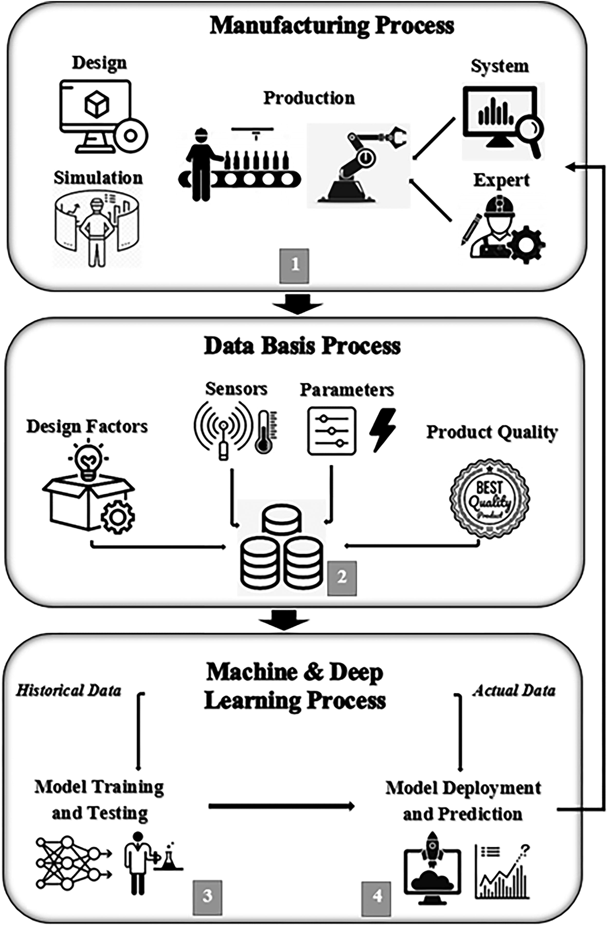
Predictive quality approach.³⁸

There are some deep learning(DL)-related studies in the literature: DL models that are based on deep Artificial Neural Network (ANN)s and that have marked major milestones in the Artificial Intelligence (AI) research in recent years. These include, for example, convolutional neural networks (CNNs) which are established in computer vision and image recognition,^18,19 as well as recurrent neural networks such as long short-term memory (LSTM) or transformer networks, which represent the state of the art in natural language processing areas such as speech recognition or machine translation.¹⁷ Ma et al. (2018) made three key contributions on their study: this study, a local processing method based on symmetric overlap-tile strategy, is adopted.²⁰

Oborski and Wysocki (2022) researched the industrial quality control system based on AI DL method. They determined that the neural network created for visual quality control of impellers of submersible pumps is characterized by a precision of 99.820%.²¹ Pan et al. (2022) used the ultrasonic elliptical vibration cutting technology for ultra-precision machining of tungsten heavy alloy. Based on the idea of DL, the surface roughness is discretized, and the fitting problem in surface roughness is transformed into a classification problem.²² Essien and Giannetti (2020) studied on an end-to-end model for multistep machine speed prediction by the motivation of recent DL studies in smart manufacturing.²³ Serin et al. (2020) reviewed and classified those studies on tool condition monitoring on their research. Firstly, tool condition monitoring, then the latest DL theories are presented, followed by insights into realizing new opportunities in tool condition monitoring.²⁴ Wang et al. (2021) identified the positive aspects of DL for solving problems such as product quality prediction in welding processes.²⁵ Zhang et al. (2019) optimized printing processes in FDM with DL.²⁶

In the study by Manoj et al., response surface methodology and artificial neural network were employed for the prediction of cutting velocity and surface roughness. Artificial neural network prediction technique was the most efficient method for the prediction of response parameters as it predicted an error percentage <6%.²⁷ In their study, Karthik et al. investigated the variation and effects of variables such as feed rate, spindle speed, cooling type and dock on Ra in face milling with different cooling techniques. The benchmark function of the proposed mode hybrid-bias (BNN–SVR) algorithm showcases the propensity to emerge out of the local minimum and coincide with the optimal target value. However, SVR surpasses BNN and RSM approaches because of the convergence factor and narrow margin error.²⁸

Lin et al. (2019) studied the efficiency of Fast Fourier Transform LSTM Network, Fast Fourier Transform-Deep Neural Networks, and one-dimensional CNN.²⁹ Dimitriou et al. (2020) propose a system that automates fault diagnosis by accurately estimating the volume of glue deposits before and even after die attachment on their research.³⁰ Li et al. (2019) presented a roughness prediction model to improve the surface integrity of additive products and concluded that the model is effective.³¹ Yun et al. (2020) proposed a vision-based system for inspecting surface defects.³² Cardoso et al. (2020) found that the MLOps approach is efficient in decision making, providing appropriate resources.³³ Klein et al. (2020) used the machine learning method of random forests to predict dimensional and surface quality characteristics of honed bores.³⁴ According to Erkan et al. glass fiber reinforced plastic composites are an economic alternative to engineering materials because of their superior properties. To reduce the number of experiments, ANN models were used to predict the damage factor.³⁵

Extreme learning machine (ELM) is originally proposed as a learning scheme for single layer feedforward networks, and it is known for being able to approximate nonlinear function by random hidden neurons. Specifically, the parameters of the hidden neurons are randomly generated, and the activation function is a nonlinear piece-wise continuous function such as sigmoid or Gaussian function. During the training, the hidden layer is not learned but the weight matrix of output layer is obtained by solving the optimization problem formulated by some learning criteria and regularizations. ELM is first designed for solving supervised learning problem, for example, classification and regression and it is then extended to unsupervised and semi-supervised learning problem by embedding the Laplacian norm in the optimization. ELM is now a generalized learning framework applied in various real-world applications, such as 3D shape analysis image classification.^{36B37 -40} A single hidden layer feedforward neural network with N-hidden nodes is defined as in equation 2. Here, a_i and b_i are the learning parameters. The i in b_i is the weight of the hidden node and G(x) is the activation function.^36,37 $f_{N} (x) = \sum_{i = 1}^{N} B_{i}, G ((a_{i}, b_{i}, x), x ϵ R, a_{i} ϵ R)$ (1)

According to the literature reviewed above, there are many studies on the effectiveness of scanning methods and 3D specimens on the dimensional accuracy and precision of products. In this study, modeling of the dimensional accuracy and precision of final products was optimized with DL and ELM methods. In this regard, it will contribute to RE studies as a theoretical and experimental study.

Materials and Method

3D printing and scanning

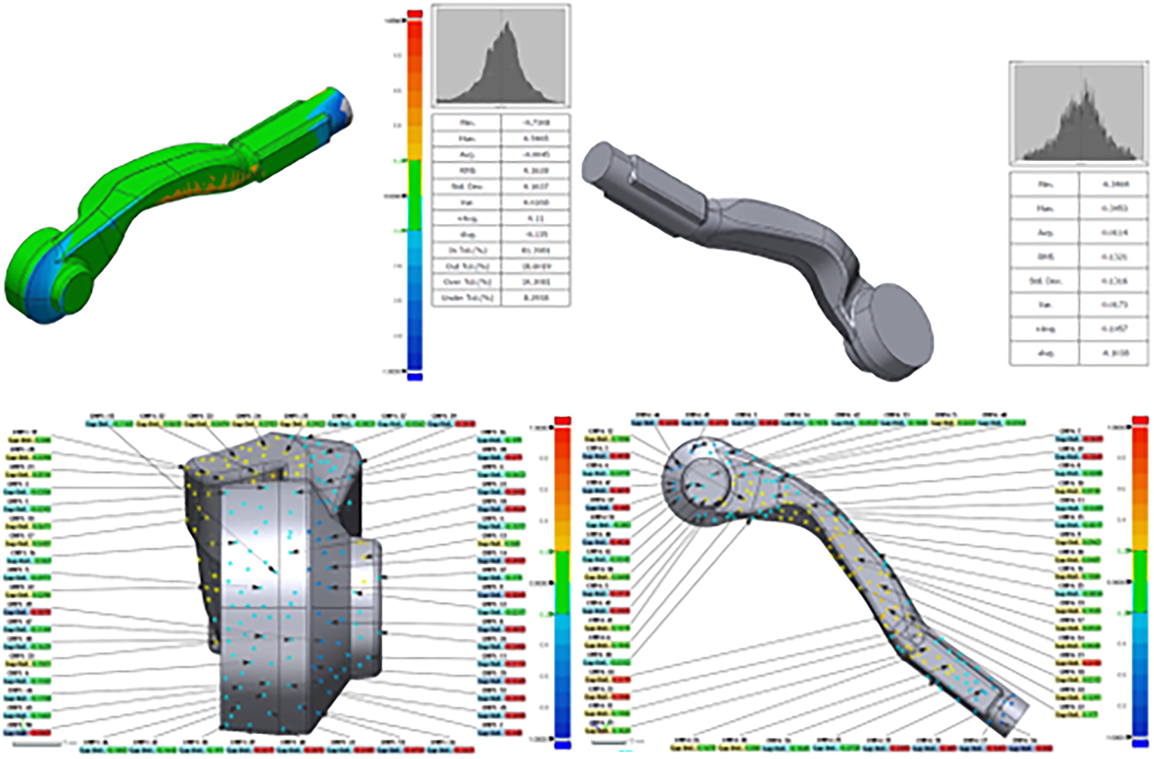
In order to demonstrate the effects of modeling methods on dimensional accuracy and precision in design and RE, a machine component was selected for the study. This component is shown in Figure 2. The 3D prototypes of the selected component were produced with the resinous system objet EDEN250 by Polyjet (Fig. 3) and the filamentous system FDM by Zortrax M200 (Fig. 4). These components were then scanned with the laser scanning device Breuckmann 3D SmartSCAN (Fig. 5). The samples were scanned from six different directions and at least 175 points were obtained in each direction. A total of 4000 points were taken in the automatic surface modeling (ASm) and parametric modeling (Pm) of the samples produced with Polyjet and FDM (Figs. 6–9). In this context, each modeling and each production method was compared with each other. This comparison revealed the differences between the nominal data given in millimeters (mm) and the scanned data.

FIG. 2.

Sample.

FIG. 3.

EDEN 250 3D printer.

FIG. 4.

Zortrax M 200 3D printer.

FIG. 5.

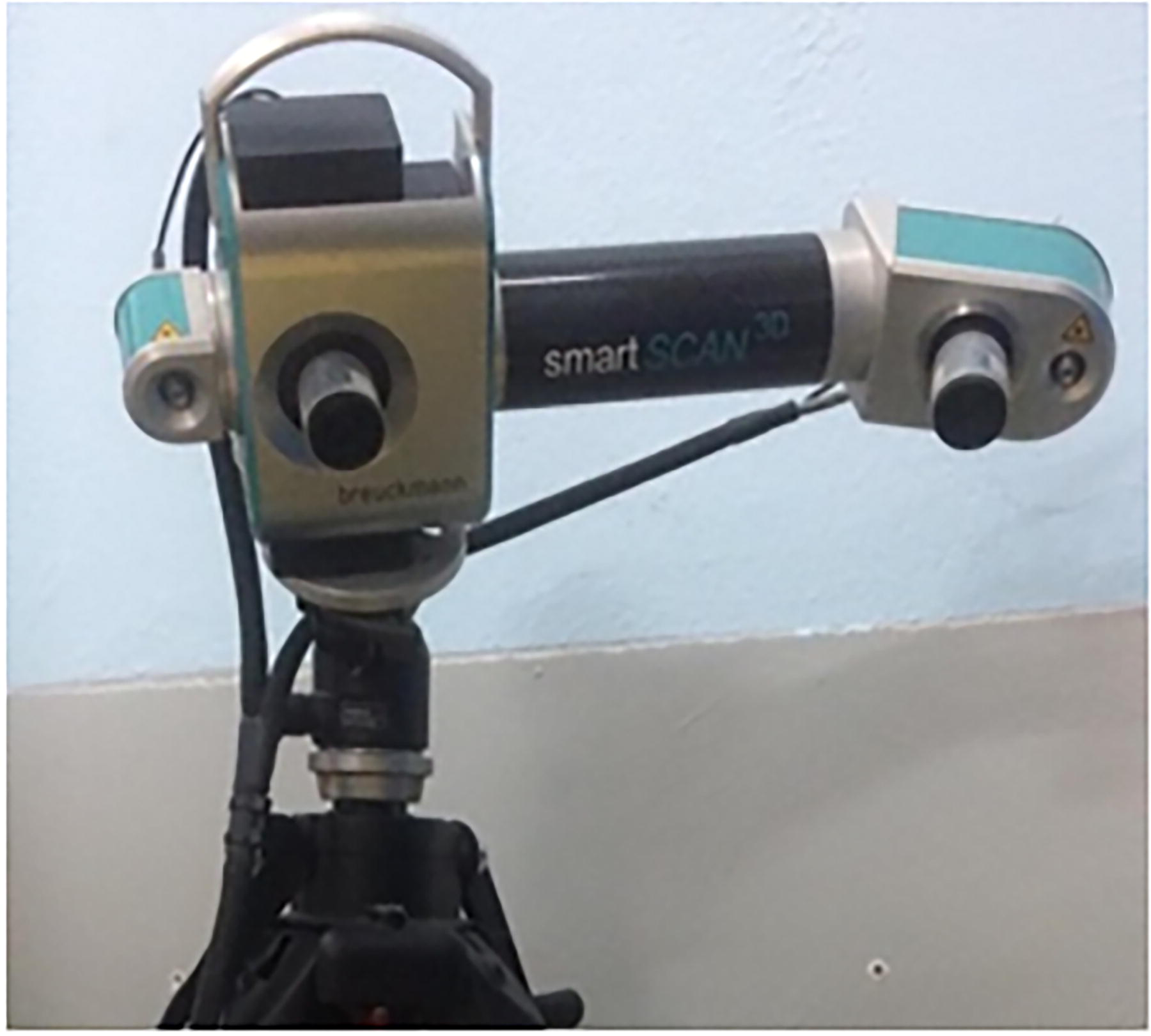
SmartSCAN 3D scanner.

FIG. 6.

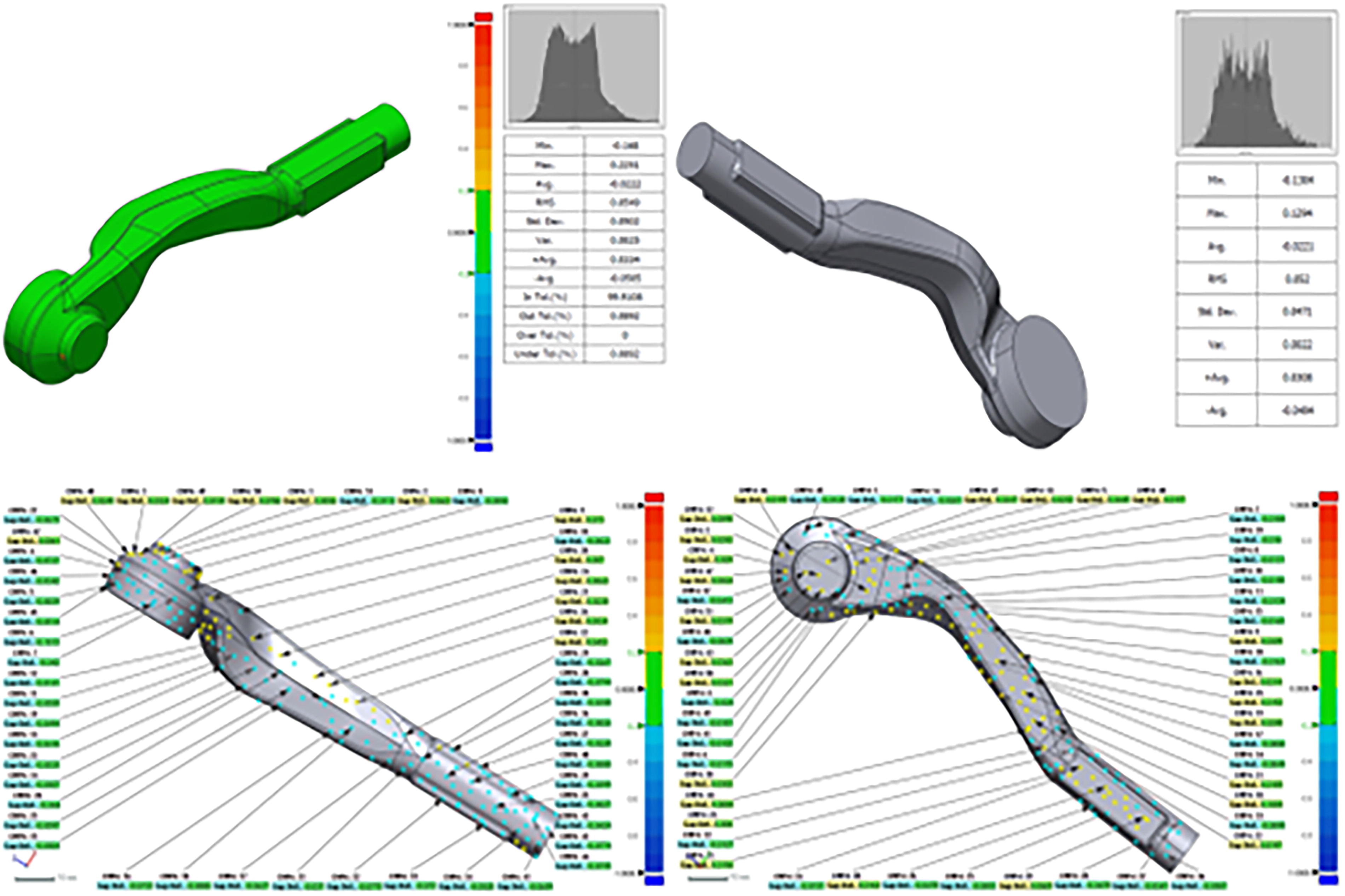
Pm (Polyjet) views. Pm, parametric modeling.

FIG. 7.

ASm (Polyjet) views. Asm, automatic surface modeling.

FIG. 8.

Pm (FDM) views.

FIG. 9.

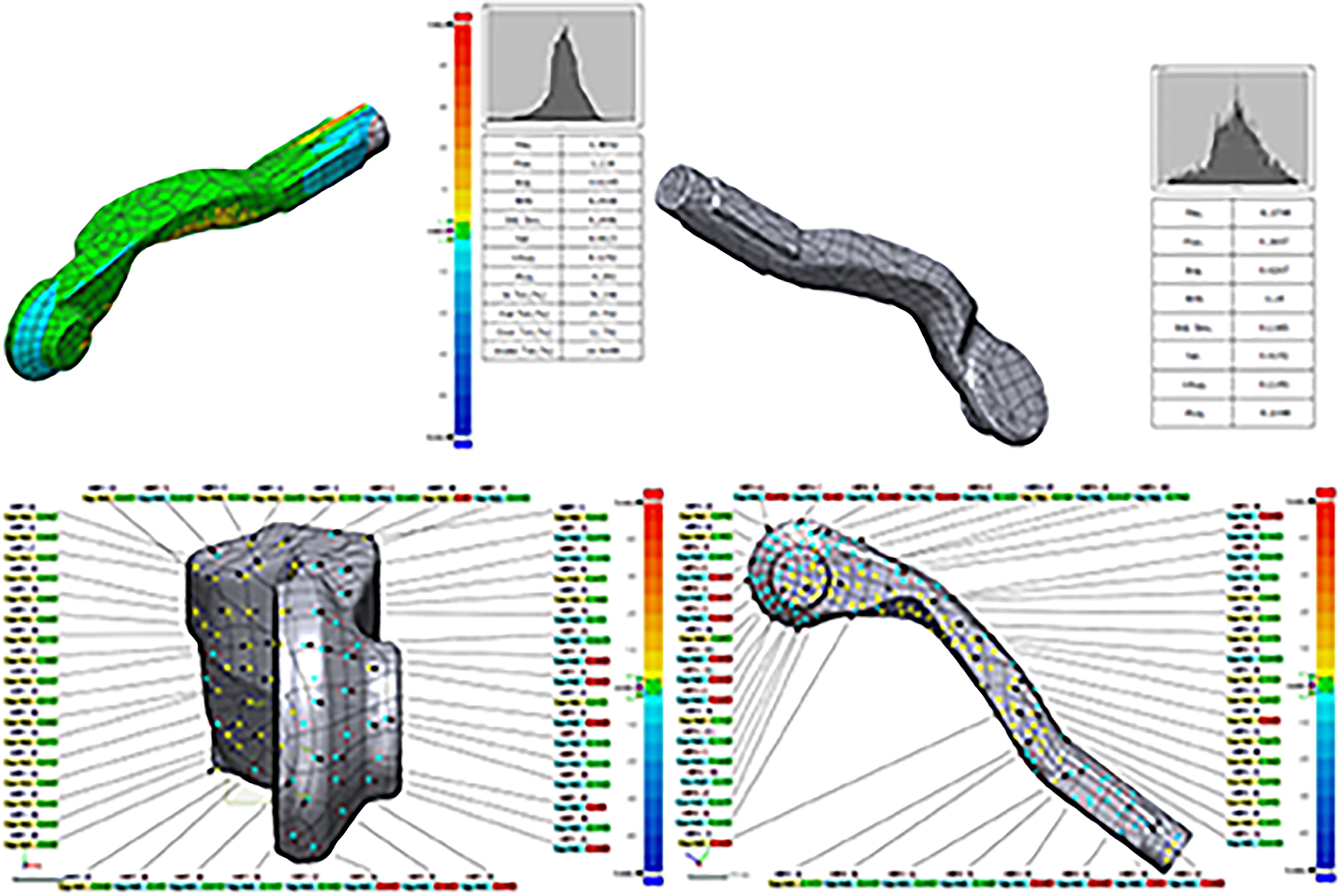
ASm (FDM) views.

The 4000 points examined in the study were obtained from three different surface structures, including plane, cylindrical, and amorphous surfaces. In the results of this study, it will be extremely important and easy to determine the modeling method according to the type of surface to be studied, depending on the data.

Modeling process

Rapidform XOR was used as software for modeling. First, polygonal data of the component was obtained by 3D scanning. Then cross sections were obtained using RE software. Two methods were applied according to the geometry of the component, accuracy and precision, cost, and the method used in modeling.

Parametric modeling

When surfaces and solids can be obtained from sketch models, each design change made on the sketches is reflected in the entire design structure.^41,42 Pm evaluates the control and update of the design and geometry with mathematical algorithms and variables. This creates a dynamic relationship between the modeling target and the model.

Auto surface modeling

This method is used to quickly edit raster data for purposes such as editing, smoothing, or sharpening polygons, removing deformations and cleaning up gaps. The difference between Pm and ASm processes is important. In Pm, the data must be obtained in a controlled manner, while in ASm, the data are generated according to the software’s own algorithm. Pm reconstructs the design changes in the whole process, regardless of the geometry. ASm is a relatively fast method for obtaining geometry. However, a dependent and specific design method like Pm can be slower in RE processes. In this context, in this study, the difference between the fast but relatively low accuracy of ASm and the high computation time of Pm is demonstrated. Furthermore, whether the surface is cylindrical, plane, or amorphous is an extremely important parameter.

Optimization process

The prediction model was created with DL and ELM for the modeling studies to be made using these data. Anaconda–Python 3.9 was used in the study. Adam and RMSProp methods as optimization algorithms, and ReLU, sigmoid, and tanh as activation functions were tried. In the experiments, the number of hidden layers was 2 and 3, and the number of neurons in each hidden layer was 10, 20, and 50. For Epochs 1000 and training, 90% and 80% of the data were determined, and for testing 10% and 20% (Table 1). A linear regression model is also presented to compare the results.

Table 1.

DL and ELM Parameters

Parameters	DL	Basic ELM	P-ELM	OP-ELM
Optimization algorithm	Adam, RMSProp	—	—	—
Normalization	Min–Max Scaling	Min–Max Scaling	Min–Max Scaling	Min–Max Scaling
Input layer activation function	ReLU, sigmoid	sigmoid	sigmoid	sigmoid
Output layer activation function	—	linear	linear	linear
Number of input layer neuron	6	6	6	6
Number of output layer neuron	1	6	6	6
Number of hidden layers	2	1	1	1
Number of hidden#1 layer neuron	10, 20	10, 20	50, 100	60, 120
Number of hidden#2 layer neuron	10, 20	—	—	—
Learning rate	0,001	—	—	—
Batch size	32
Training size	0.8	0.8	0.8	0.8
Test size	0.2	0.2	0.2	0.2
Epochs	500	—	—	—

DL, deep learning; ELM, extreme learning machines; OP-ELM, optimized with ELM.

Result and Discussion

Optimization with DL and ELM

Optimization is a mathematical discipline that determines the best solution in a quantitatively well-defined sense. The mathematical optimization of processes governed by partial differential equations has made significant progress over the past decade and has since been applied to a wide variety of disciplines such as science, engineering, mathematics, economics, and even commerce. Optimization theory provides algorithms and analysis of these algorithms to solve well-structured optimization problems. An optimization problem contains an objective function that will be minimized or maximized with given constraints. Optimization theory provides algorithms and analysis of these algorithms to solve well-structured optimization problems. Stochastic gradient-based optimization is of fundamental practical importance in many fields of science and engineering. Many problems in these fields can be posed as optimization of some scalar parameterized objective function that requires maximization or minimization according to its parameters.

In this study, 36 different studies were tried with these DL parameters. In addition, 12 different studies were tried with these ELM parameters. The DL and ELM model used in the study are shown in Figure 10. The dataset for DL and ELM are set to 4000. Based on the mean squared error (MSE), the most effective results were determined with Adam as optimization algorithm, ReLU as activation function, number of hidden layers 2, number of neurons 20, and 10% of the data for testing. As a result, the lowest MSE of 1.011 × 10⁻⁶ was obtained in DL.

FIG. 10.

(A) DL architecture of this study. (B) ELM architecture of this study. DL, deep learning; ELM, extreme learning machines.

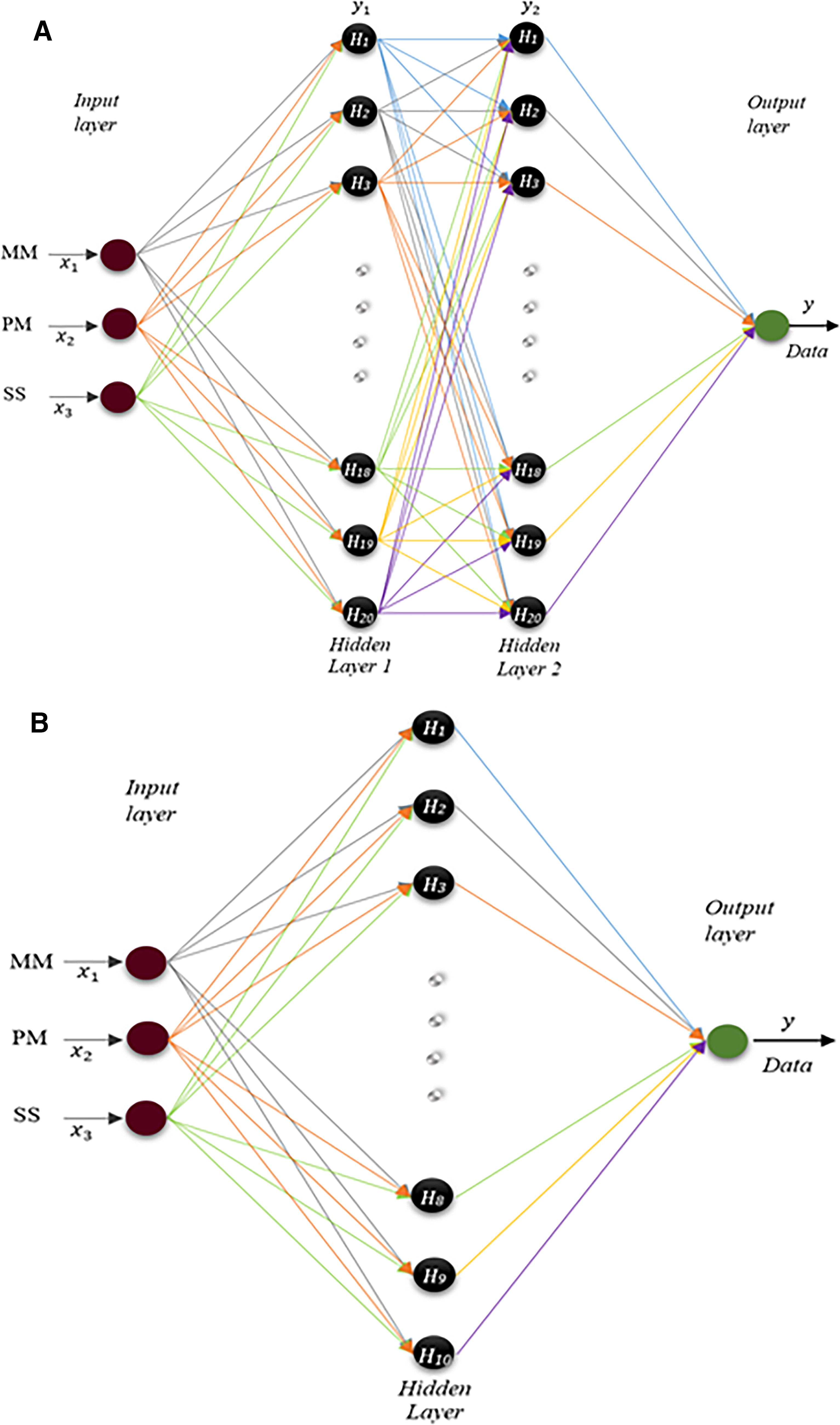
In this study, the activation function is sigmoid in the hidden layer and linear in the output layer for ELM. The number of neurons in the hidden layer was determined as 10, 20, 50, 60, 100, and 120 and the number of neurons in the output layer was determined as 1. These results were optimized with ELM, the MSE value was 1.011 × 10⁻⁶, and the r² value was 0.9748. This shows that ELM gave very successful prediction results as the most effective optimization.

A linear regression model is also presented to compare the results. This can be understood as an indication of high accuracy prediction. The R-square values of DL were given and comparison was made possible (Table 2). It has also been optimized with DL and ELM linear regression to compare the optimization results. The results are given in Table 2. In linear regression, MSE value was calculated as 1.484 × 10⁻⁶ and r² value as 0.9677. This shows that ELM gave very successful prediction results as the most effective optimization. In addition, the regression model equation of dependent and independent variables is shown in equation 1.

y = - 0,0203 + 0,00033 * MM + 0.00063 * PM - 0,00017 * SS

(2)

Table 2.

Results of DL and ELM

	Method	Optimization algorithms methods	Neuron numbers	Activation functions	Training MSE	Test MSE	r ²
Data	Linear regression				1.531 × 10⁻⁶	1.484 × 10⁻⁶	0.9677
	Deep learning	Adam	10, 10	ReLU, ReLU	1.347 × 10⁻⁶	1.203 × 10⁻⁶	0.9265
			10, 10	tanh, tanh	1.485 × 10⁻⁶	1.339 × 10⁻⁶	0.9134
			Sigmoid, Sigmoid	1.318 × 10⁻⁶	1.241 × 10⁻⁶	0.8649
			20, 20	ReLU, ReLU	1.206 × 10⁻⁶	1.161 × 10⁻⁶	0.9774
			20, 20	tanh, tanh	1.295 × 10⁻⁶	1.257 × 10⁻⁶	0.9281
		Sigmoid, Sigmoid	1.279 × 10⁻⁶	1.248 × 10⁻⁶	0.8924
		RMSProp	10, 10	ReLU, ReLU	1.466 × 10⁻⁶	1.213 × 10⁻⁶	0.9141
			10, 10	tanh, tanh	1.371 × 10⁻⁶	1.214 × 10⁻⁶	0.8923
			Sigmoid, Sigmoid	1.185 × 10⁻⁶	1.176 × 10⁻⁶	0.8296
			20, 20	ReLU, ReLU	1.259 × 10⁻⁶	1.172 × 10⁻⁶	0.8469
			20, 20	tanh, tanh	1.179 × 10⁻⁶	1.172 × 10⁻⁶	0.8827
	Sigmoid, Sigmoid	1.504 × 10⁻⁶	1.209 × 10⁻⁶	0.9128
	ELM	Basic ELM	10	Sigmoid	1.038 × 10⁻⁶	1.023 × 10⁻⁶	0.9358
		20	1.034 × 10⁻⁶	1.018 × 10⁻⁶	0.9469
		P-ELM	50	Sigmoid	1.031 × 10⁻⁶	1.021 × 10⁻⁶	0.9514
		100	1.029 × 10⁻⁶	1.022 × 10⁻⁶	0.9588
		OP-ELM	60	Sigmoid	1.027 × 10⁻⁶	1.019 × 10⁻⁶	0.9697
120	1.021 × 10⁻⁶	1.011 × 10^-6	0.9748

MSE, mean squared error.

ASm in products produced with Polyjet gave better results than Pm in general on surfaces. In addition, this result implicates the validity of the improvement work. The results may act as a guide for the use of DL and ELM in new projects (Fig. 11).

FIG. 11.

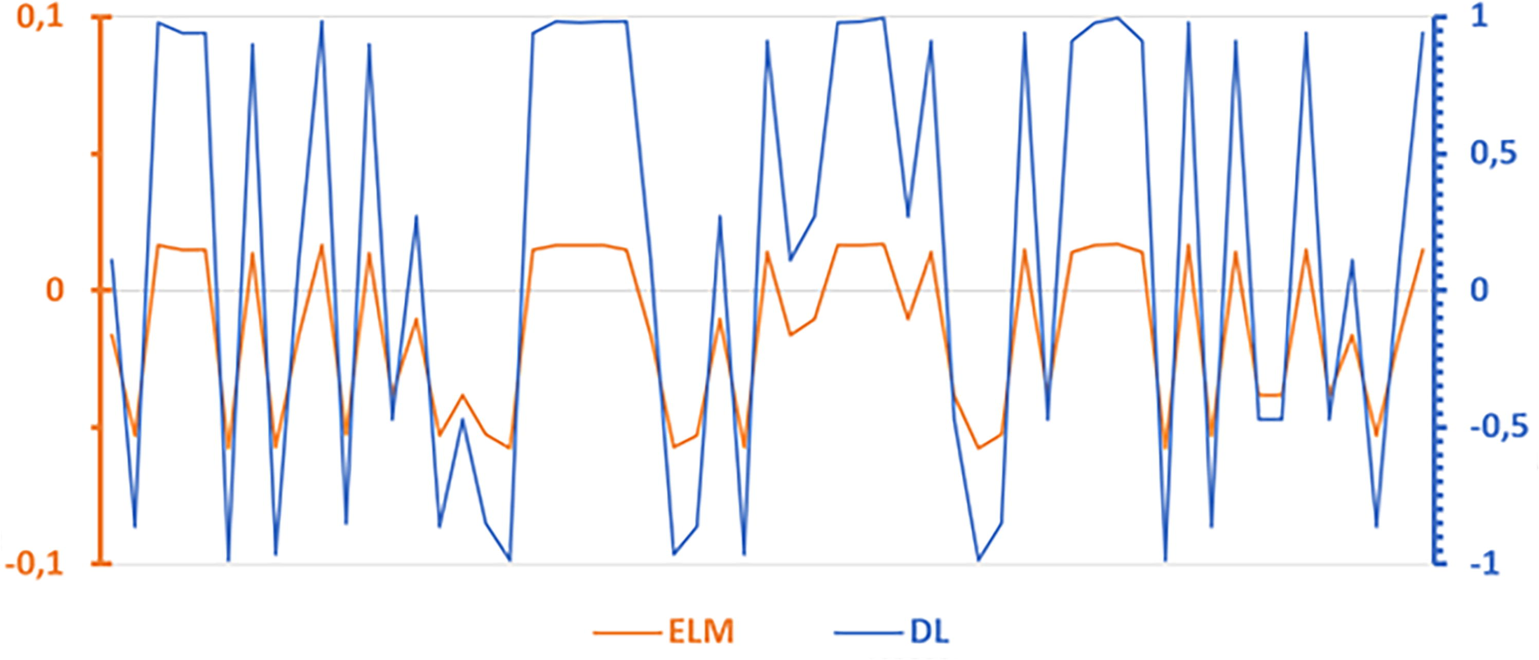
Comparison of ELM and DL test values.

Conclusions

The study aimed to reveal the effects of modeling method on dimensional accuracy and precision in design and analysis and the results were obtained in this context. The difference in dimensions of 3D models produced by Polyjet and FDM using ASm and Pm was examined. According to the DL and ELM made because of scanning the plane, cylindrical, and amorphous components, the following results were obtained. •

The performance of the model created in DL and ELM were quite close to the actual performance. This result implicates the validity of the improvement work.

•

The most effective results with DL optimization were determined with Adam as optimization algorithm, ReLU as activation function, number of hidden layers 2, number of neurons 20, and 20% of the data for testing. As a result, the lowest MSE of 1.011 × 10⁻⁶ was obtained in DL. The DL r² value was set to 0.9774. The results may act as a guide for the use of DL in new projects.

•

But these results are optimized with the ELM. The MSE value was calculated as 1.011 × 10⁻⁶ and the r² value was 0.9748. It has also been optimized with linear regression to compare the DL and ELM optimization results. The MSE value was calculated as 1.484 × 10⁻⁶ and r² value as 0.9677.

•

This shows that ELM gave very successful prediction results as the most effective optimization.

Footnotes

Acknowledgment

The author would like to express his thanks and gratitude to the Dean's Office of the Faculty of Engineering of 19 Mayıs University for opening its doors to him and providing him with an academic study environment and opportunities after the devastating earthquakes in the southeast of Turkey on 6 February 2023. The author would also like to thank ‘Poligon Engineering/Istanbul’ for their support.

Author’s Contribution

As a single author, the entire work (a) conceptualization and data curation, (b) investigation and methodology, and (c) writing—original draft and writing—review and editing are performed by the author.

Author Disclosure Statement

No competing financial interests exist.

Funding Information

No funding was received for this article.

References

1. Altuğ

. A Comparıson study ın terms of dımensıonal accuracy and precısıon of 3D modeling. Int J Innov Eng Appl 2022;6(1); doi: 10.46460/ijiea.1012067

2. Palanisamy

, Raman

, Dhanraj Kumar

. Additive Manufacturing: A Review on Mechanical Properties of Polyjet and FDM Printed Parts. Springer: Berlin Heidelberg; 2022; doi: 10.1007/s00289-021-03899-0

3. Monzón

, Ortega

, Martínez

, et al. Standardization in additive manufacturing: Activities carried out by international organizations and projects. Int J Adv Manuf Technol 2015;76(5–8):1111–1121; doi: 10.1007/s00170-014-6334-1

4. Singh

, Ramakrishna

, Singh

. Material issues in additive manufacturing: A review. J Manuf Process 2017;25:185–200; doi: 10.1016/j.jmapro.2016.11.006

5. Goh

, Agarwala

, Goh

, et al. Additive manufacturing in unmanned aerial vehicles (UAVs): Challenges and potential. Aerosp Sci Technol 2017;63:140–151; doi: 10.1016/j.ast.2016.12.019

6. Armillotta

, Bianchi

, Cavallaro

, et al. Edge quality in fused deposition modeling: II. experimental verification. Rpj 2017;23(4):686–695; doi: 10.1108/RPJ-02-2016-0021

7. Mantada

, Mendricky

, Safka

. Parameters influencing the precision of various 3D printing technologies. Mm Sj 2017;2017(05):2004–2012; doi: 10.17973/MMSJ.2017_12_201776

8. Maurya

, Rastogi

, Singh

. Comparative study and measurement of form errors for the component printed by FDM and polyjet process. I2M 2019;18(4):353–359; doi: 10.18280/i2m.180404

9. Dietrich

, Ender

, Baumgartner

, et al. A validation study of reconstructed rapid prototyping models produced by two technologies. Angle Orthod 2017;87(5):782–787; doi: 10.2319/01091-727.1

10.

10. Cheng

, Zhang

, Biyikli

, et al. Efficient design optimization of variable-density cellular structures for additive manufacturing: Theory and experimental validation. Rpj 2017;23(4):660–677; doi: 10.1108/RPJ-04-2016-0069

11.

11. Anwer

, Mathieu

. From reverse engineering to shape engineering in mechanical design. CIRP Ann 2016;65(1):165–168; doi: 10.1016/j.cirp.2016.04.052

12.

12. van Eijnatten

, Berger

, de Graaf

, et al. Influence of CT parameters on STL model accuracy. Rpj 2017;23(4):678–685; doi: 10.1108/RPJ-07-2015-0092

13.

13. Aroca

, Ventura

CEH

, De Mello

, et al. Sequential additive manufacturing: Automatic manipulation of 3D printed parts. Rpj 2017;23(4):653–659; doi: 10.1108/RPJ-02-2016-0029

14.

14. Doubenskaia

, Grigoriev

, Zhirnov

, et al. Parametric analysis of SLM using comprehensive optical monitoring. Rapid Prototyp J 2016;22(1):40–50; doi: 10.1108/RPJ-04-2014-0046

15.

15. Isa

, Lazoglu

. Design and analysis of a 3D laser scanner. Measurement 2017;111:122–133; doi: 10.1016/j.measurement.2017.07.028

16.

16. Wang

, Feng

. Effects of scanning orientation on outlier formation in 3D laser scanning of reflective surfaces. Opt Lasers Eng 2016;81:35–45; doi: 10.1016/j.optlaseng.2016.01.003

17.

17. Tercan

, Meisen

. Machine learning and deep learning based predictive quality in manufacturing: A systematic review. J Intell Manuf 2022;33(7):1879–1905; doi: 10.1007/s10845-022-01963-8

18.

18. Szegedy

, Liu

, Jia

, et al. Going deeper with convolutions. In: 2015 IEEE Conference on Computer Vision and Pattern Recognition (CVPR) IEEE; 2015; pp. 1–9; doi: 10.1109/CVPR.2015.7298594

19.

19. Redmon

, Divvala

, Girshick

, et al. You only look once: Unified, real-time object detection. In: 2016 IEEE Conference on Computer Vision and Pattern Recognition (CVPR) IEEE; 2016; pp. 779–788; doi: 10.1109/CVPR.2016.91

20.

20. Ma

, Ban

, Huang

, et al. Deep learning-based ımage segmentation for Al-La alloy microscopic ımages. Symmetry (Basel) 2018;10(4):107; doi: 10.3390/sym10040107

21.

21. Oborski

, Wysocki

. Intelligent visual quality control system based on convolutional neural networks for holonic shop floor control of ındustry 4.0 manufacturing systems. Adv Sci Technol Res J 2022;16(2):89–98; doi: 10.12913/22998624/145503

22.

22. Pan

, Kang

, Dong

, et al. On-line prediction of ultrasonic elliptical vibration cutting surface roughness of tungsten heavy alloy based on deep learning. J Intell Manuf 2022;33(3):675–685; doi: 10.1007/s10845-020-01669-9

23.

23. Essien

, Giannetti

. A deep learning model for smart manufacturing using convolutional LSTM neural network autoencoders. IEEE Trans Ind Inf 2020;16(9):6069–6078; doi: 10.1109/TII.2020.2967556

24.

24. Serin

, Sener

, Ozbayoglu

, et al. Review of tool condition monitoring in machining and opportunities for deep learning. Int J Adv Manuf Technol 2020;109(3–4):953–974; doi: 10.1007/s00170-020-05449-w

25.

25. Wang

, Jiao

, Wang

, et al. A tutorial on deep learning-based data analytics in manufacturing through a welding case study. J Manuf Process 2021;63(December 2019):2–13; doi: 10.1016/j.jmapro.2020.04.044

26.

26. Zhang

, Wang

, Gao

. Deep learning-based tensile strength prediction in fused deposition modeling. Comput Ind 2019;107:11–21; doi: 10.1016/j.compind.2019.01.011

27.

27. Manoj

, Soni

, Narendranath

, et al. Examination of machining parameters and prediction of cutting velocity and surface roughness using RSM and ANN using WEDM of Altemp HX. Adv Mater Sci Eng 2022;2022;2022:1–9; doi: 10.1155/2022/5192981

28.

28. Karthik

RMC

, Malghan

, Kara

, et al. Influence of Support Vector Regression (SVR) on cryogenic face milling. Adv Mater Sci Eng 2021;2021(1); doi: 10.1155/2021/9984369

29.

29. Lin

W-J

, Lo

S-H

, Young

H-T

, et al. Evaluation of deep learning neural networks for surface roughness prediction using vibration signal analysis. Appl Sci 2019;9(7):1462; doi: 10.3390/app9071462

30.

30. Dimitriou

, Leontaris

, Vafeiadis

, et al. Fault diagnosis in microelectronics attachment via deep learning analysis of 3-D laser scans. IEEE Trans Ind Electron 2020;67(7):5748–5757; doi: 10.1109/TIE.2019.2931220

31.

31. Li

, Zhang

, Shi

, et al. Prediction of surface roughness in extrusion-based additive manufacturing with machine learning. Robot Comput Integr Manuf 2019;57(October 2018):488–495; doi: 10.1016/j.rcim.2019.01.004

32.

32. Yun

, Shin

, Koo

, et al. Automated defect inspection system for metal surfaces based on deep learning and data augmentation. J Manuf Syst 2020;55(May 2019):317–324; doi: 10.1016/j.jmsy.2020.03.009

33.

33. Cardoso Silva

, Rezende Zagatti

, Silva Sette

, et al. Benchmarking machine learning solutions in production. In: 2020 19th IEEE International Conference on Machine Learning and Applications (ICMLA) IEEE; 2020; pp. 626–633; doi: 10.1109/ICMLA51294.2020.00104

34.

34. Klein

, Schorr

, Bähre

. Quality prediction of honed bores with machine learning based on machining and quality data to ımprove the honing process control. Procedia CIRP 2020;93:1322–1327; doi: 10.1016/j.procir.2020.03.055

35.

35. Erkan

, Işık

, Çiçek

, et al. Prediction of damage factor in end milling of glass fibre reinforced plastic composites using artificial neural network. Appl Compos Mater 2013;20(4):517–536; doi: 10.1007/s10443-012-9286-3

36.

36. Huang

, Liu

, Yang

, et al. Discriminative clustering via extreme learning machine. Neural Netw 2015;70:1–8; doi: 10.1016/j.neunet.2015.06.002

37.

37. Huang

, Huang

, Bin

Song S

, et al. Trends in extreme learning machines: A review. Neural Netw 2015;61:32–48; doi: 10.1016/j.neunet.2014.10.001

38.

38. Liu

, Liyanaarachchi Lekamalage

, Huang

, et al. Extreme learning machine for joint embedding and clustering. Neurocomputing 2018;277:78–88; doi: 10.1016/j.neucom.2017.01.115

39.

39. Wang

, Xie

, Xu

, et al. An efficient and effective convolutional auto-encoder extreme learning machine network for 3d feature learning. Neurocomputing 2016;174:988–998; doi: 10.1016/j.neucom.2015.10.035

40.

40. Chen

, Li

, Zhou

. Process parameters appraisal of fabricating ceramic parts based on stereolithography using the Taguchi method. Proc Inst Mech Eng Part B J Eng Manuf 2012;226(7):1249–1258; doi: 10.1177/0954405412442607

41.

41. Zhang

, Zhong

, Wu

, et al. 3D parametric modeling of complex geological structures for geotechnical engineering of dam foundation based on T-Splines. Computer Aided Civil Eng 2018;33(7):545–570; doi: 10.1111/mice.12343

42.

42. Buonamici

, Carfagni

, Furferi

, et al. Reverse engineering of mechanical parts: A template-based approach. J Comput Des Eng 2018;5(2):145–159; doi: 10.1016/j.jcde.2017.11.009