
Abstract
In reviewing manuscripts or in reading published research studies, the reader should always ask about the appropriateness of statistical methods. For the clinician, a clear algorithm will usually remove a lot of the guesswork when deciphering statistical language. Most studies submitted to medical journals, unless they are large population outcomes studies targeting novel metrics, can be analyzed using time-tested, universally understood methods. The intent of this article is to help the clinician perform an initial screen for appropriateness of the statistic methods chosen by the investigators.
Introduction
I
The final caution about statistics goes back to the first statement of it being a way to organize and interpret our observations of events. How meaningful the final statistic calculations are depends on how well the observations are captured by the study design before being entered into the “number crunching machine.” The old adage of “garbage, in garbage out” certainly holds true here. The author of this article frequently uses the example of studying the contributors of reflux but weeding out the “broccoli.” While there may be 100 potential variables (including the like or dislike of broccoli) that may seemingly be associated with reflux (e.g., p<0.05), the investigators need to perform due diligence upfront to determine the most reasonable or plausible causes to capture, even if it seems like the severity of reflux may be associated with whether the patient likes broccoli. However, negative data are still worth looking into deeper because new discoveries are often the outliers. Remember that strong statistical inferences toward a certain result are never absolute, and should stand the test of other statistical methods, prospective testing, corroboration by other investigators, and, most importantly, common sense. Always ask, even though the statistics suggest a certain result, whether it is believable and practical.
Statistic Algorithm
When reviewing a paper, it is common to read over the abstract to determine if it falls in your area of interest and expertise, as well as the magnitude of clinical impact from such a study. Regardless of whether the study is randomized, blinded, retrospective, or prospective, the questions to ask include:
• Is it comparing differences between certain groups? • Is it studying a treatment and effect (e.g., Is drug X effective in causing diabetes remission)? • Is it comparing the differences in outcome between two different treatments (e.g., gastric banding vs. sleeve gastrectomy)? • Is it studying the causal relationship of a certain observation (e.g., Is the severity of gastroesophageal reflux affected by body mass index)?
If the investigators cannot be clear about the questions they are asking, the statistics will likely be murky and subject to greater scrutiny. After understanding the questions being asked by the study, it makes sense to refer immediately to the end of the Methods section (which is often the last paragraph). Ignore the types of statistical machinery that were used (e.g., SAS, SPSS, Excel, Statistica, R, etc.) because these are simply proprietary tools that are the favorite weapons of the investigators. Focus on the inclusion and exclusion criteria, how they treat missing data, and the statistical method being used (analysis of variance, linear regression, Wilcoxon, chi-square, etc.). So the reader should try to connect the question itself by a straight line with the actual method, and make sure there are no “breaks” in the line.
For years, the author has had an algorithm tree by David C. Howell at hand to help determine if the statistics makes sense. 1 You will need to refer to it frequently in this article. Multiple similar versions have been strewn around the Internet, but this author has modified and adapted the algorithm, and will call it the Howell Decision Tree (Fig. 1).a Complete credit goes to Dr. Howell for its origin.
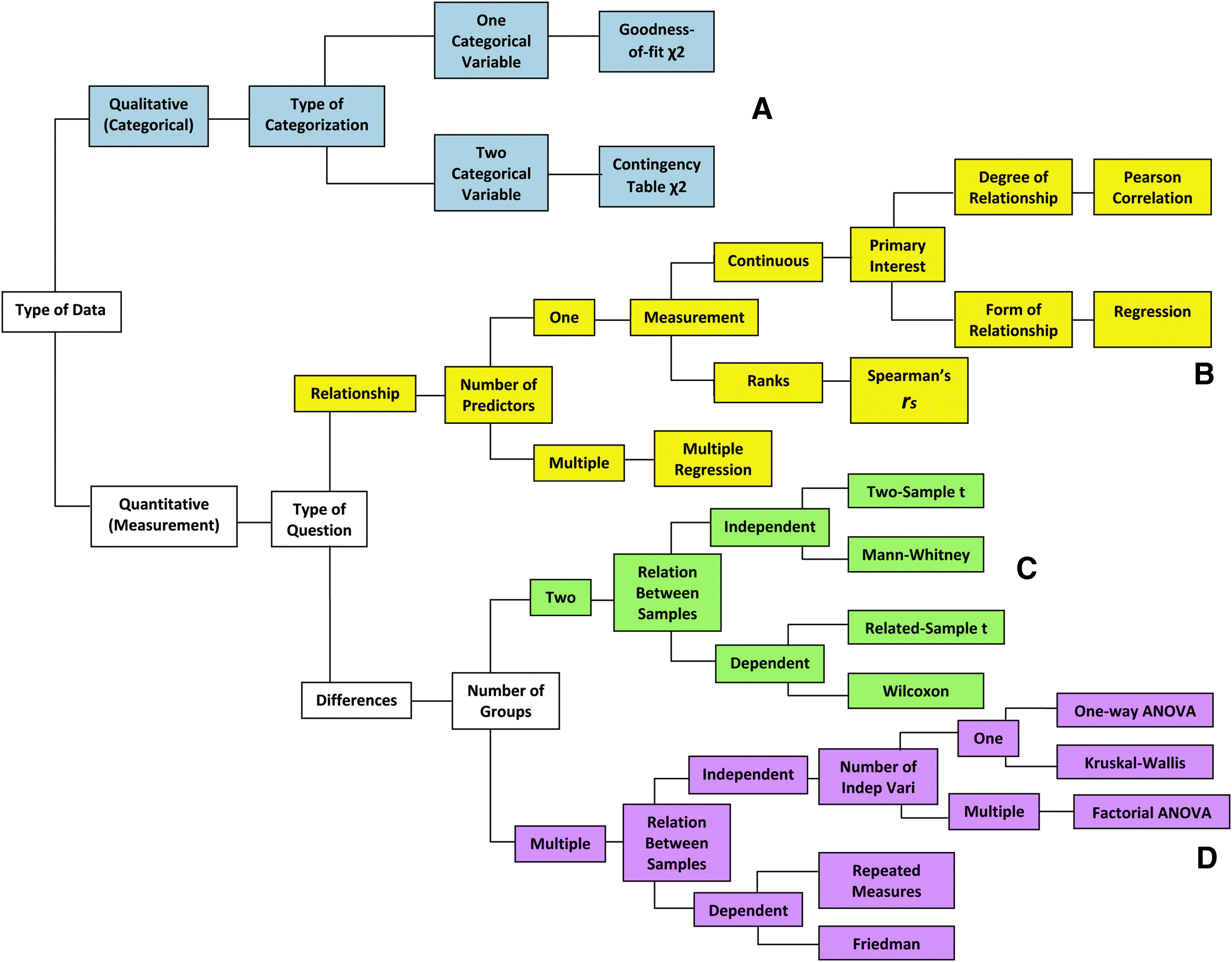
Howell Decision Tree, 2004, with four branches
What types of data are being presented?
Qualitative data
Are the data of the “yes or no” variety, such as pregnant or not pregnant, obese or not obese? (Some may refer to them as binary variables because they are either 0 or 1.) If so, these are called “qualitative” or “categorical” data and are generally uncomplicated, and should follow the uppermost branch of the of the decision tree (Fig. 1A) leading to a chi-square test. They are frequently presented as ratios or percentages. In small sample sizes (i.e., <20), a Fisher's exact test serves the same purpose. In a study to determine the likelihood of a woman conceiving based on a certain body mass index (BMI), it is appropriate to use a one-categorical variable and proceed to a goodness-of-fit chi square (unfortunately also known as Pearson's chi square, which can be confused with the correlation by the same name; read below). If the study compares the pregnancy rate between two different BMI ranges such as <30 kg/m2 and >40 kg/m2, a contingency (association) table chi square can be used. Contemporary statistics software will usually automatically sort that out during calculations without much manipulation. Some people refer to categorical data as “count” or “frequency” data because they count how often a certain event happens in each category, such as 20 women with morbid obesity had complicated pregnancies, while 10 women with normal BMI experienced the same problem.
Quantitative data
Any data that are numeric measurements such as weight changes, waist circumference, blood loss volume, length of hospital day, and size of hiatal hernia are quantitative or continuous data. While this is a simplistic explanation, it is important to make the early association that the use of the Pearson correlation, regression analysis, Mann–Whitney, or analysis of variance (ANOVA) is for numeric measurements or continuous data.
Is there a relationship between one factor and another?
If the investigators attempt to determine if an observation (also known as a dependent variable) is caused by a single particular factor (independent variable), a calculation can be performed to determine if a univariate causal relationship exists, which follows the upper middle branch of the decision tree (Fig. 1B). So if a study seeks to determine if the number of gastric band adjustments in a year affects the degree of weight loss, a statistics program will automatically generate the degree of relationship between these two variables known as the correlation (r), which is a point between −1 and +1. It is tempting to say that r=0.63 means a 63% correlation, but mathematicians will strongly rebuke that interpretation because r only tells you the strength of a relationship and whether it is positive or negative. From a clinical standpoint, an r>0.80 or <−0.80 has been accepted as a strong correlation, but it is rare to see this level of correlation in clinical practice. The notation of r2 is what one would describe if an outcome could be explained by the cause being studied. So a correlation coefficient of r=0.63 would translate into an r2 of 40%, which means that the frequency of band adjustments can explain the degree of weight loss only 40% of the time. The other 60% of weight loss must be the result of other variables. You can hopefully see why an r<0.50 would be deemed weak because r2 is only 25%.
If the same question of band adjustment frequency is ranked, where 1 would be between zero and three adjustments a year, 2 would be between four and six adjustments a year, 3 would be between seven and nine adjustments a year, 4 would be 10–12 adjustments a year, and 5 would be 13–20 or more adjustments a year, the data would be presented as a Spearman's correlation (rs). You will likely get the same results by using the Pearson correlation for Spearman's rank.
More sophisticated research typically looks to identify several clinically relevant variables that may cause a certain effect. For example, one may ask to find all the factors that may contribute to the success of an adjustable gastric band as measured by weight loss. These possible contributing (independent) variables may include income level, marital status, number of child dependents, traveling distance, frequency of band adjustments, frequency of support group visits, and so on. In this case, a multiple regression or multivariable analysis is performed by the statistics software. The final output will generally offer a relative weight of contribution by each factor, some more important and others less, toward the degree of weight loss. Multiple regressions are one of the most commonly used tools to construct predictive models for clinical outcomes such as determinants of optimal weight loss in band patients, or morbidity risks from bariatric surgeries.
In studies that determine the odds of an outcome happening, a logistic regression is used, which is similar to any linear regression, except that the outcomes is usually a “yes or no” categorical outcome (cure or disease, pregnant or not pregnant, dead or alive), and the contributing variable is a numeric measurement like laboratory values. For example, a post gastric bypass patient may or may not have a marginal ulcer depending on the frequency of tobacco smoking. The more cigarettes smoked per week (on the x-axis of a graph) may increase the likelihood of developing a marginal ulcer (on the y-axis), and such results are usually reported as odds ratio with confidence intervals.
Is there a difference in outcomes?
In looking at differences in weight loss at 1 year between the adjustable gastric band and a vertical sleeve gastrectomy, it is reasonable to follow the lower middle branch of the decision tree (Fig. 1C) that leads to a t-test, Mann–Whitney, or Wilcoxon signed-rank test. If a test is on related samples—which is the same as repeated measures, dependent samples, and paired samples—it only means that the same patient is being studied before and after treatment. An example would be to compare hunger scores before and after a sleeve gastrectomy in the same patients. A variant of this would be a matched pairs test where patients with identical characteristics undergo one or the other treatment at the same time. A straightforward t-test assumes normal (bell-curve) distribution of the study population, and a Wilcoxon signed-rank test makes no such assumption of any distribution (nonparametric). Again, software programs will give both results, which will probably be the same. However, being able to distinguish the nuances tells the reader that the investigators know what they are doing.
If the samples are unrelated or independent, such as comparing hunger scores between two groups of patients, one undergoing medical management and the other undergoing sleeve gastrectomy for morbid obesity, a two-sample t-test can be performed, but this assumes that the patient distributions are normal. A more clinically realistic study realizes that the populations may not be normally distributed (nonparametric), and hence the Mann–Whitney test for differences in outcomes between a treatment group and a control group, or between drug A and drug B, is a frequent tool in medical efficacy trials.
To determine differences between multiple (three or more) groups of interventions or treatments, or changes over time, ANOVA should be used (lowermost branch of the decision tree, Fig. 1D). The one-way ANOVA is used when you wish to find differences between three or more independent (unrelated) groups as a result of a one-time treatment. An example is to see the effect on 3-month hemoglobin A1c levels in four different treatment groups—(a) medical management, (b) adjustable banding, (c) sleeve gastrectomy, and (d) gastric bypass—to determine if there are differences. The test simply tells you there is a difference somewhere in this group, and a post hoc analysis is then carried out by the software to determine where the differences lie. There are several post-hoc procedures, but the easiest one we have used is the Tukey test. If the one-way ANOVA fails to demonstrate a difference, it is not appropriate to perform a post hoc analysis in an attempt to discover some difference. If additional layers of treatments are used in addition to the surgical procedures, such as the addition of probiotics to the four treatment groups, this now becomes a two-way (or multiple factor if even more treatments are added on) ANOVA. Finally, the Kruskal–Wallis test is simply the nonparametric variant of the one-way ANOVA.
The repeated-measures ANOVA is for related (or dependent) patient groups, where the different treatments are applied to the same group of patients. The study can be designed to measure post prandial plasma ghrelin levels in the same patients after gastric bypass operations over three or more different time points, say, 0 months, 1 month, and 6 months. Another study that utilizes repeated-measures ANOVA may measure ghrelin levels at the first physician encounter, 3 months following medical management, and 3 months after gastric bypass. In this way, longitudinal evaluation is provided for three or possibly more treatments in the same patient. Logistically, this type of study is probably the most challenging, albeit powerful, because of the time requirements and higher potential for missing data resulting from patient attrition. The Friedman test, if used at all, is the nonparametric variant of the repeated-measures ANOVA.
In general, a t-test examines the differences between two groups, while ANOVA examines differences between any number of groups of two or greater. An ANOVA can be performed with two test groups, but multiple t-tests should not be performed in place of ANOVA due to additive effects of type 1 errors for each test performed (i.e., increasing false positives).
Examples
The following are real examples taken from the literature, which might highlight how statistic procedures are routinely used.
(1) Schauer et al. 1 randomized 150 type 2 diabetic patients to intensive medical management or surgical management plus intensive surgical management to determine which would lead to greater reduction in glycated hemoglobin below 6% twelve months after treatment. They used the chi-square test to analyze the primary endpoint of 12% resolution in the medical management group, compared with 42% resolution in the combined treatment group. For continuous laboratory measurements, ANOVA was used, and for change from baseline, a repeated-measures ANOVA was used since the patients were followed over time.
(2) Lin and Gletsu-Miller 2 studied the effects of Roux-en-Y gastric bypass on the longitudinal effects of various glycemic parameters, including insulin secretion, insulin uptake, HOMA index, and physical adiposity over a 24 month period. There was a significant improvement in glycemic status in patients at 24 months, but significant improvements were noted by 6 months after surgery. Repeated-measures ANOVA was used to determine differences between groups over time, followed by post hoc comparisons using Tukey's test. On occasion, a paired t-test was used for differences between time points within the same group, but the authors conceded in the Methods section that this was less conservative (because of additive type 1 errors). Relationships between age, glycemic status, and race/ethnicity were determined by multiple regression analysis. An unpaired t-test was performed to compare outcomes of those in the group who completed 24 months of the study and those who only completed the first 6 months. However, one can argue that an ANOVA would also suffice for this last comparison. To compare the proportions of glycemic status with race, a chi square analysis was used.
(3) Greenstein et al. 3 used the Longitudinal Assessment of Bariatric Surgery database to determine the factors associated with adverse intraoperative events during obesity surgery. The rates of adverse events for laparoscopic gastric banding, laparoscopic gastric bypass, and open gastric bypass were compared using the Pearson chi-square test (also known as the goodness-of-fit chi-square test). Fisher's exact test was used to determine the association between adverse events frequency and major complications, which makes the assumption that the incidence was low. Indeed, the incidence of these complications was less than 10%. A multivariable relative risk model (a multiple regression) was used to determine the degree in which different factors contributed to complications.
(4) Aithal et al. 5 randomized nondiabetic patients with nonalcoholic steatohepatitis (NASH) to placebo or Pioglitazone for 12-months. At the end of the study period, the treatment group exhibited improved metabolic and liver histology parameters. As you might anticipate, the Mann–Whitney U-test was applied to compare the groups. The paired t-test was used for normally distributed data, and the Wilcoxon signed-rank test was used for nonparametric data.
Conclusion
Statistical methods in the medical literature need not be a mystery, and the above examples serve as a foundation before venturing into more complex statistical methods. We are surrounded by professional statisticians and bioinformatics athletes, as well as “couch statisticians” who know just enough to critique the plays. Possessing a frame of reference, such as the Howell Decision Tree, increases familiarity with the language and serves as an effective screening tool for the appropriateness of the statistics being used. The Internet is also loaded with statistics definitions and practical references that can help any person overcome the language barriers of statistics. Frequent use of a statistical framework, as with learning a foreign language, eventually becomes effortless. Finally, never sacrifice common sense and your professional clinical acumen for unfamiliar statistical vernacular or powerful statistic tools.
Footnotes
Acknowledgment
The author gratefully acknowledges William Knechtle, MPH in the Emory Department of Surgery Quality & Outcomes Office for reviewing this article.
Disclosure Statement
No competing financial interests exist.
Notes
a. David Howell is Professor Emeritus in Psychology at the University of Vermont and former chairman of that department. The author has used this decision tree by Howell since 2004, but cannot find that particular version to properly cite it.