A Data Snapshot Approach for Making Real-Time Predictions in Basketball

Abstract

This article proposes a novel approach, called data snapshots, to generate real-time probabilities of winning for National Basketball Association (NBA) teams while games are being played. The approach takes a snapshot from a live game, identifies historical games that have the same snapshot, and uses the outcomes of these games to calculate the winning probabilities of the teams in this game as the game is underway. Using data obtained from 20 seasons worth of NBA games, we build three models and compare their accuracies to a baseline accuracy. In Model 1, each snapshot includes the point difference between the home and away teams at a given second of the game. In Model 2, each snapshot includes the net team strength in addition to the point difference at a given second. In Model 3, each snapshot includes the rate of score change in addition to the point difference at a given second. The results show that all models perform better than the baseline accuracy, with Model 1 being the best model.

Introduction

Your favorite basketball team is trailing by 10 points at the beginning of the fourth quarter. Should you accept a possible defeat and perhaps do something else, or should you continue watching and hope for a comeback? For more than 30 years, this question has garnered the interest of many researchers. Numerous methodologies have been proposed to generate live or in-game predictions to not only quell the curiosity of basketball enthusiasts but also inform coaches and support staff in helping them devise strategies during gameplay. Most of these methodologies suffer from limitations ranging from inadequate data to restrictive assumptions. The goal of this study is to propose an alternative approach—referred to as data snapshots—that can provide live predictions during gameplay based on the characteristics of the game.

In the section that follows, we discuss prior approaches that can generate live predictions in basketball games. Then, we describe the approach developed in this study, present our analyses, and discuss the applications of this approach to other domains outside of sports.

Background

One of the earliest nonparametric approaches that can generate the in-game winning probabilities of the home and away teams utilizes the lead at the end of the first and third quarters of a game to calculate the winning probabilities.¹ Using data collected from 200 National Basketball Association (NBA) games in the 1990–1991 season, the study reports that if a team is leading at the end of the first quarter, it has a 69.8% probability of winning the game. This increases to 79.84% if the team is leading at the end of the third quarter. Note that this approach does not consider the magnitude of the lead, only its presence.

Another nonparametric approach extended this work by focusing on the comparison between the point difference between the teams and the remaining time on the game clock.² The study offers two models based on NBA games in the 2006–2007 season. The first model selects the leading team as the winner if the team's lead (in point difference) is greater than the time (in minutes) left on the game clock (e.g., team A will be the winner if it has a 5-point lead in the last 4 minutes of the game). The second model—aimed at making earlier predictions during the game—looks at the same comparison, but this time divides the time remaining on the clock by two. In this case, the model calls team A the winner if it has a 5-point lead in the last 9 minutes of the game. The model accuracies are 93.2% and 89.1%, respectively. Despite their impressive accuracies, these models cannot handle a tie at the end of a quarter. Furthermore, the models provide only one prediction (when the condition is satisfied first) and do not revise their prediction if the other team satisfies the same condition later in the game.

Previous work also offers parametric approaches to generate in-game predictions. Stern³ fits a Brownian motion model on the point differences observed at the end of four quarters. The model uses 493 NBA games played in 1992 and generates the probabilities of winning for the different point differences observed at the end of each quarter. For example, a 5-point lead at the end of the third quarter translates into a 78% probability of winning for the leading team.

In another parametric study, a probabilistic model is proposed, which is based on the assumption that scores are normally distributed.⁴ The model uses the NBA games in the 1997–1998 season and breaks down the probabilities for home and away teams separately. Thus, a home team's winning probability is 85% if it has a lead at the end of the third quarter. However, this is only 79% for the away team due to the home team's court advantage.

Building on these models, recent work is based on Markov models, which track the progression of games and predict winners. For example, Shirley⁵ uses certain game statistics (such as ball possession, the method by which the possession is gained, and points scored on the previous possession) as the states of the Markov chain. The model—based on 4.5 games in the 2006–2007 season—shows that as the number of transitions left in the game decreases, the home team's chances of winning increases. Similarly, Štrumbelj and Vračar⁶ use a Markov model and extend Shirley's work by including more states into the model. They also compare their model to other statistical models, such as a logit regression and a latent strength-ranking model, as well as bookmaker odds. Although their model achieves an accuracy of 69%, other models achieve accuracies ranging from 67% to 69%. Vračar et al.⁷ later extend this work by incorporating all in-game events and the transition time between two consecutive events into the Markov model.

Apart from Markov models, previous work also focuses on autoregressive, latent trajectory, and autoregressive latent trajectory models by using the point differences between home and away teams at the end of each quarter.⁸ The findings show that an autoregressive model best fits the data, and a logistic regression achieves an accuracy of 72% when predicting the winner.

More recently, regression discontinuity has been used with variables such as the point difference between the teams at halftime and whether a team is losing at halftime or not.⁹ Based on data collected from 18,060 NBA games between the 1993–2009 seasons, the model shows that the chances of winning increase (between 5.8% and 8%) if a team is behind at halftime.

As summarized above, there is considerable work on generating live (or in-game) probabilities of winning for home and away teams. However, prior approaches suffer from several limitations. First, some of the models rely on only a few data points per game. Second, certain models do not lend themselves to a tie at the end of a quarter, let alone an overtime. Third, parametric models make assumptions that limit their applicability. For example, the homogeneity of time or of point differences undermines the generalizability of the Markov models.⁷ Finally, comparing models across studies and identifying the best model are difficult because most studies do not evaluate the goodness of their models; they only report the probabilities generated by the models.

In this article, we develop a novel approach that addresses these concerns while putting the practicality and applicability of the model to the forefront. The next section describes this approach in detail.

Data Snapshot Approach

Our approach relies on capturing a snapshot from a live game (while the game is underway) and comparing this snapshot to snapshots obtained from historical games to generate the winning probabilities of the home and away teams in the live game. Our unit of time is a second; therefore, a snapshot includes the attributes of a game at a given second of the game. This leads to 2880 snapshots for a typical NBA game without overtime (4 quarters × 12 minutes × 60 seconds), where each snapshot captures the game attributes at that second of the game. Games with overtime have more snapshots because of the overtime seconds. At a minimum, the game attributes must include the point difference between the home and away teams. However, other information, such as team strength or rate of score change, can also be considered as other salient game attributes.

After capturing the most current snapshot from a live game (using the desired set of game attributes), the algorithm searches for historical games that have the exact same snapshot. The outcomes of the historical games are then used to generate the winning probabilities of the home and away teams in the live game for this specific snapshot. The identification of the historical games is performed by setting the Euclidean distance between the current snapshot and historical snapshots to 0. That is, the algorithm searches for historical snapshots that are the same as the snapshot captured from the live game. If each game is considered to be a separate time-series data set, our approach can be likened to earlier work on time-series classification. However, although prior work identifies the similarity between two time-series data sets using the Euclidean distance or dynamic time warping (see Ratanamahatana and Keogh's¹⁰ work for a review), our similarity measure relies on setting the Euclidean distance to 0 (and therefore searching for exact matches in the historical snapshots). So instead of identifying historical games that are similar to the current game, we identify historical games that have exactly the same snapshot as the one obtained from the current game. Then, we use the outcomes of these historical games to generate the winning probabilities in the current game.

Consider the following example: imagine a game where the home team has a 5-point lead at the 10-minute 30-second mark in the first quarter. If the only game attribute considered in the snapshot is the point difference between the two teams, then the snapshot is defined as 5 points (in favor of the home team) at 10 minutes 30 seconds in the first quarter. The algorithm identifies all historical games that have the matching snapshot (i.e., 5 points in favor of the home team at 10 minutes 30 seconds in the first quarter). Then, the algorithm calculates the proportion of wins by home teams among these games. This is the probability of winning the current game for the home team for this specific snapshot. For example, the model may find 100 historical games in which the home teams have a 5-point lead at 10 minutes 30 seconds in the first quarter. If 70 of these games were won by the home teams, then the probabilities of winning for the home and away teams are calculated as 70% and 30%, respectively, at 10 minutes 30 seconds in the first quarter. The pseudocode of this algorithm is presented in Figure 1.

FIG. 1.

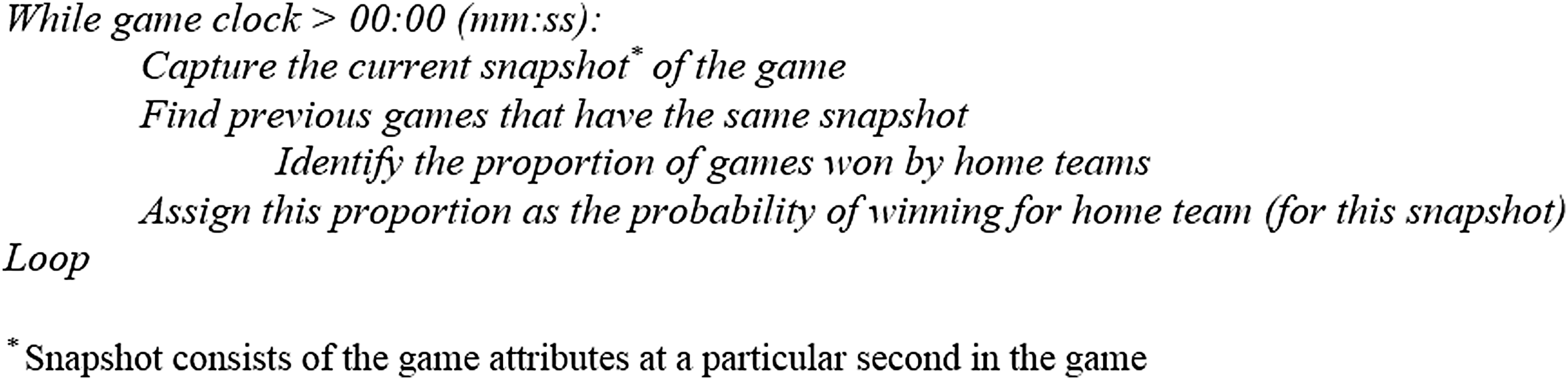
Pseudocode of the data snapshot approach.

Unique snapshots

It is possible that a snapshot obtained from the current game may be unique and that the algorithm may not find matching snapshots in the historical games. Although this can be mitigated by having as many historical games as possible—so that all possibilities are accounted for—the algorithm should still accommodate unique snapshots. To this end, we relax the restriction, the Euclidean distance. If the algorithm identifies a unique snapshot, it uses a nearest neighbor approach by searching for the two nearest point differences observed in that second, S, of the game. For example, if there are no matching snapshots for a 5-point difference (in favor of the home team) at 10 minutes 30 seconds in the first quarter, the algorithm uses the 6-point and the 4-point differences (based on their availability) at 10 minutes 30 seconds in the first quarter. The outcomes of these games are then used to calculate the winning probabilities. Note that the nearest snapshots can be one or more points away, depending on what is observed in the historical games. Furthermore, the nearest snapshots are based only on the point difference. That is, the algorithm keeps the game time lines the same and does not search for nearest snapshots at S + 1 or S−1 since we consider each S a disparate state in the game time line.

Model Evaluation

Our approach generates the winning probability of each team for each of the 2880 snapshots during a game. To calculate the overall accuracy of the model, we combine the 2880 probability predictions made during a game and compare this to the game outcome using the Brier score originally proposed by Brier.¹¹

The Brier score is commonly used for atmospheric sciences, such as meteorology and climatology, to evaluate model goodness.¹² It helps evaluate the probability forecasts of events that have binary outcomes. As seen in Equation (1), it requires two variables: the probability of the occurrence of an event \documentclass{aastex}\usepackage{amsbsy}\usepackage{amsfonts}\usepackage{amssymb}\usepackage{bm}\usepackage{mathrsfs}\usepackage{pifont}\usepackage{stmaryrd}\usepackage{textcomp}\usepackage{portland, xspace}\usepackage{amsmath, amsxtra}\usepackage{upgreek}\pagestyle{empty}\DeclareMathSizes{10}{9}{7}{6}\begin{document} $$\left( {{y_k}} \right)$$ \end{document} and the real outcome of the event \documentclass{aastex}\usepackage{amsbsy}\usepackage{amsfonts}\usepackage{amssymb}\usepackage{bm}\usepackage{mathrsfs}\usepackage{pifont}\usepackage{stmaryrd}\usepackage{textcomp}\usepackage{portland, xspace}\usepackage{amsmath, amsxtra}\usepackage{upgreek}\pagestyle{empty}\DeclareMathSizes{10}{9}{7}{6}\begin{document} $$\left( {{o_k}} \right)$$ \end{document} . Although the probability is a continuous value between 0 and 1, the outcome is binary: it is “1” if the event occurs and “0” if it does not. In essence, the Brier score is the mean squared error of the probability forecasts. For example, consider a model that forecasts a 70% chance of rain for tomorrow. Here, the model has a Brier score of 0.09 if it actually rains [as per Equation (1), where y₁ = 0.70, o₁ = 1, and n = 1]. Consider a second forecast made a few hours later that increases the chance of rain to 80%. Now, the model—based on these two forecasts—generates a Brier score of 0.065 if it indeed rains [as per Equation (1), where y₁ = 0.70, y₂ = 0.80, o₁ = 1, o₂ = 1, and n = 2]. Therefore, models that have a Brier score closer to 0 are better than models that have a Brier score closer to 1 (i.e., a Brier score of 0 indicates a perfect model). \documentclass{aastex}\usepackage{amsbsy}\usepackage{amsfonts}\usepackage{amssymb}\usepackage{bm}\usepackage{mathrsfs}\usepackage{pifont}\usepackage{stmaryrd}\usepackage{textcomp}\usepackage{portland, xspace}\usepackage{amsmath, amsxtra}\usepackage{upgreek}\pagestyle{empty}\DeclareMathSizes{10}{9}{7}{6}\begin{document} \begin{align*} { \rm { Brier \;score } } = \frac { 1 } { n } \sum \nolimits_ { k = 1 } ^n { \left( { { y_k } - { o_k } } \right) ^2 } \tag { 1 } \end{align*} \end{document}

The Brier score is particularly useful for our purpose because the data snapshot approach described earlier generates 2880 probabilities (more if there is overtime) for each game, where the outcome is binary (win or lose). Therefore, we assess the model's accuracy using the Brier score formula presented in Equation (1).

Data Set

Our data set consisted of 23,532 NBA games played between the 1996 and 2016 seasons (20 seasons), excluding the playoff games. To build our data set, we downloaded the play-by-play data of each of these games from http://stats.nba.com. Note that the play-by-play data of a game is an event-based breakdown of that game from start to finish (see Fig. 2 for an example).

FIG. 2.

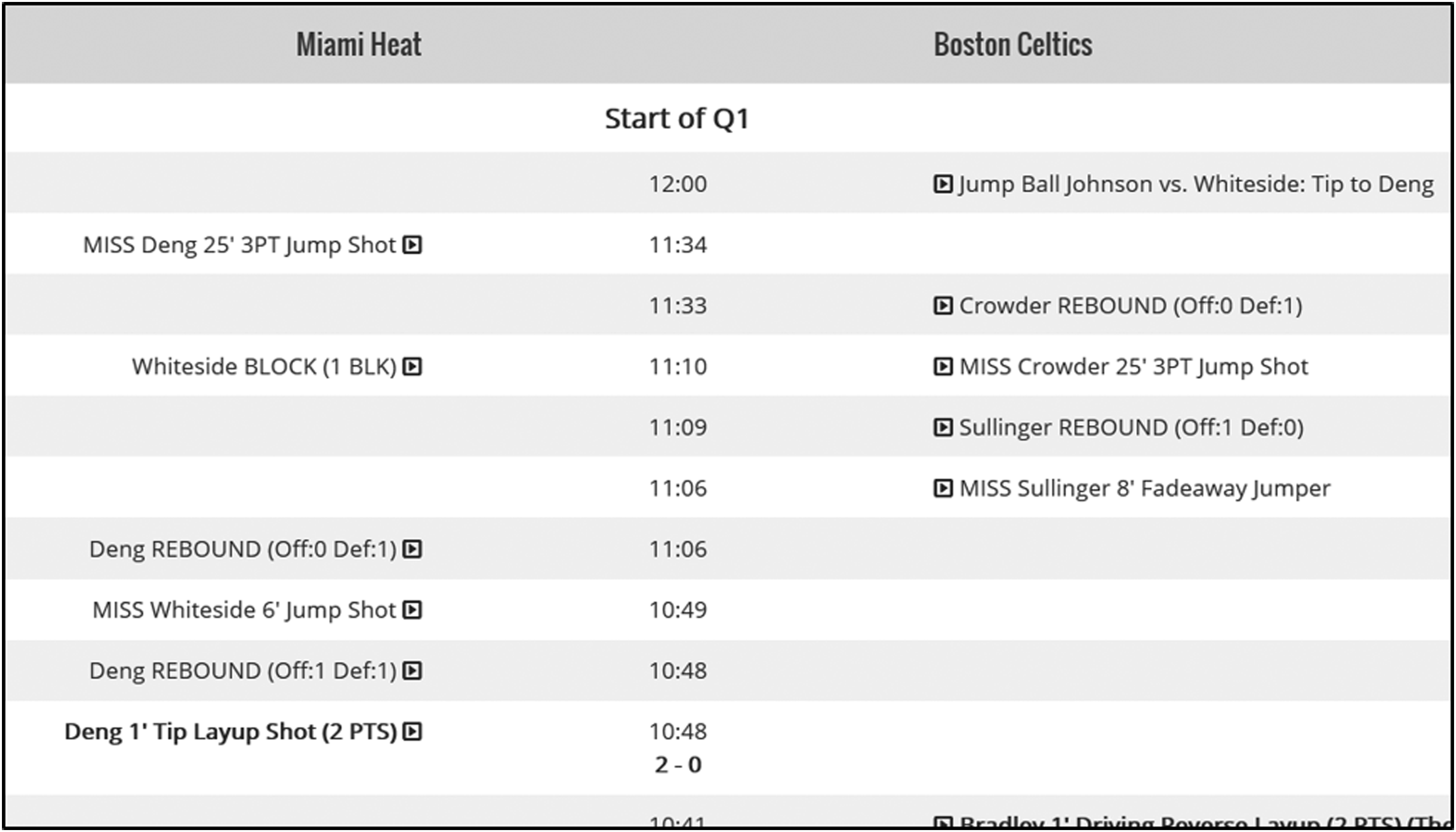
Example of play-by-play data.

Play-by-play data include only significant in-game events (such as rebounds, shots, and fouls), along with the event's description, time, and impact on the score. If there is no significant event during gameplay, then there is a time gap between the previous event and the next event. For example, as seen in Figure 2, the game starts at 12 minutes 0 seconds, and the first event is reported at 11 minutes 34 seconds as a jump shot. Therefore, there is a 26-second gap in between the first two events. Also, as seen in Figure 2, the play-by-play data show the game score only if a team scores any points. For example, the game score is displayed at 10 minutes 48 seconds (as 2-0) for the first time because of a field goal scored by the Miami Heat.

To create our data snapshots, we wrote a script that looked at the play-by-play data of each game in our data set and expanded it to encompass each second of that game, regardless of whether there was an event at that second or not. Therefore, for each game, we generated a continuous time line second-by-second along with the game score at each second.

Thus, we had 2880 snapshots for each game (if there was no overtime), with each snapshot showing the time of the snapshot, the game attributes at that snapshot (such as the point difference between the home and away teams), and the winner of the game. Note that games that went into overtime had more snapshots, depending on the overtime minutes played. In total, we had 68,398,501 snapshots in our data set. This constituted our training data set.

We further created a similar data set for the 1230 games (excluding playoffs) of the 2016–2017 regular season. This constituted our validation set.

Baseline Accuracy

We calculated our baseline accuracy based on the in-game lead. We assumed that if a team was leading at a specific second of the game, it had a 100% probability of winning, and if it was trailing at another second of the game, it had a 0% probability of winning. If there was a tie at a given second of the game, we assigned a 50% probability of winning to each team. This generated an average Brier score of 0.264 (with a standard deviation of 0.250) on the 1230 games of the validation set.

To account for home court advantage, we created a second baseline using the same approach but with a modified probability for ties: if there was a tie at a given second, the home team had a 59.8% probability of winning. This was motivated by the fact that 14,084 of the 23,532 games (or 59.8%) in the training set were won by home teams. This generated the same average Brier score and the same standard deviation.

We also created different versions of these baselines by assigning winning probabilities ranging from 70% to 90% (with 10% increments) to the leading team using 50% and 59.8% probabilities for ties. (We tried a 60% probability of winning as well, but this caused higher Brier scores.) These generated baselines ranging from 0.224 (with a standard deviation of 0.201) to 0.200 (with a standard deviation of 0.101).

We also considered using the findings of prior work as possible baselines. However, this turned out challenging because prior work did not report game- or season-based Brier scores. Although it was possible to derive Brier scores based on certain findings, these scores would not have been meaningful because our Brier scores took every second of a game into account, whereas these scores would have been derived from a single point in the game time line. Nonetheless, the baseline approaches discussed above should still be a good proxy for some of the findings reported in earlier work (especially those by Cooper et al.,¹ Stern,³ and Berger and Pope,⁹ which provide probabilities of winning for the leading team at specific points in the game).

Therefore, among these baselines, the lowest value was 0.200 (with a standard deviation of 0.101) generated by a 70% winning probability for the leading team (at a given second) and 59.8% probability for the home team if there was a tie (at a given second). We used this value to evaluate our models.

Model 1

In this model, our snapshots included only the point difference observed between the home and away teams for each second of a game. We followed the procedure described earlier in the Data Snapshot Approach section. That is, we identified the first snapshot of the first game in the validation set. Then, we found the matching snapshots in the training set. We used the outcomes of these games to calculate the winning probabilities of the home and away teams for this snapshot of the first game in the validation set. We then repeated this for all snapshots of all games in the validation set. As a result, we calculated a separate Brier score for each of the 1230 games in the validation set.

Results

This model generated a maximum Brier score of 0.722 and a minimum score of 0.009 for the 1230 games in the validation set. The average Brier score of these games was 0.170 (with a standard deviation of 0.133), which was lower than the baseline accuracy value of 0.200.

Figure 3 shows the predictions made by this model for an example game in the validation set. The left vertical axis of the figure shows the predicted probabilities of winning, while the right vertical axis shows the point difference observed. The x-axis shows the game time line in seconds. As seen in the figure, the model predicts winning probabilities in accordance with the point differences observed during the game.

FIG. 3.

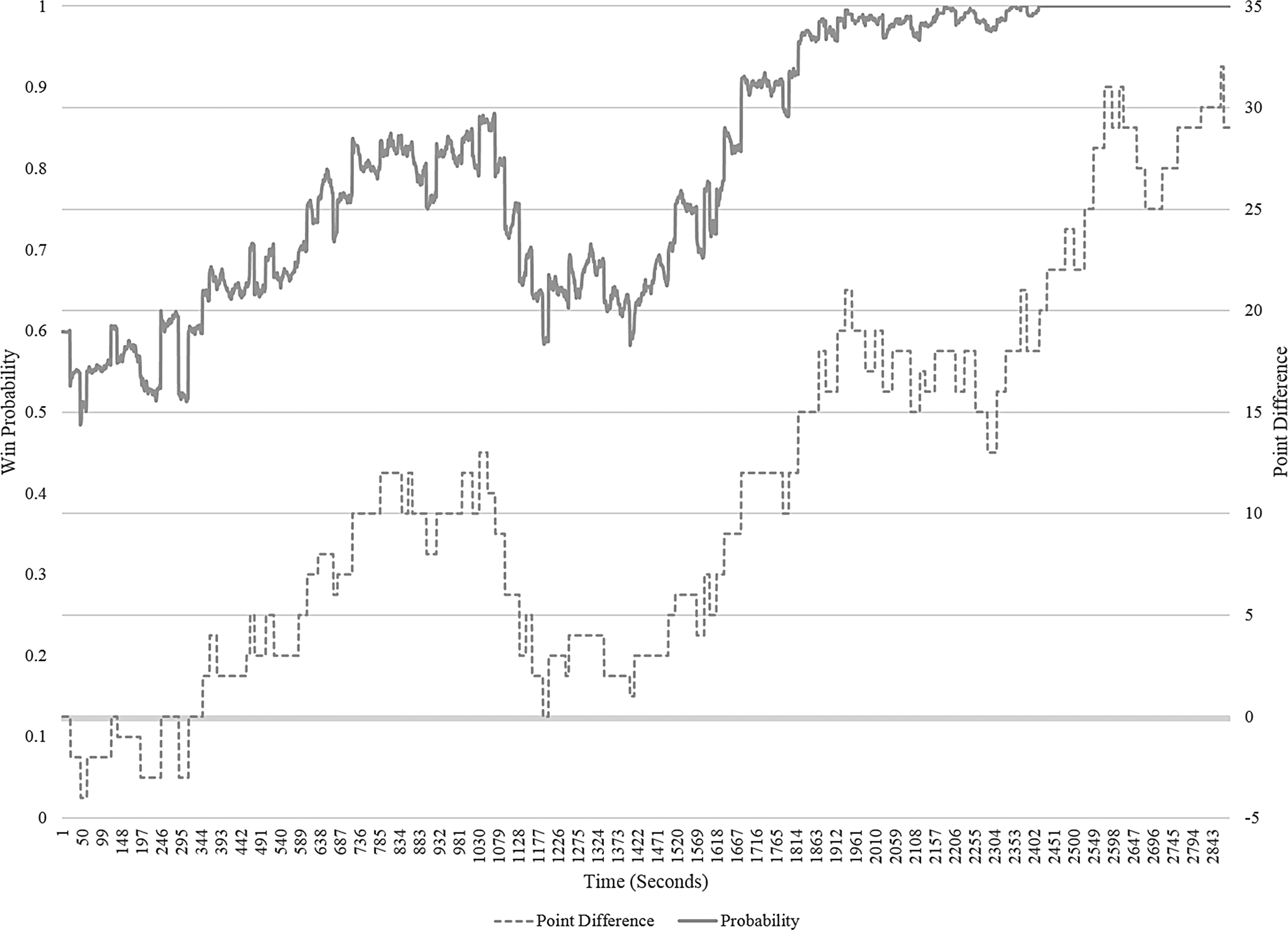
Probability predictions of an example game.

To see if the results were particular to the 2016–2017 season or not, we conducted a “leave-one-season-out” approach using the training data set. Accordingly, we used one of the seasons (such as the 2000–2001 season) as the holdout sample and used the remaining 20 seasons as the training set (from the 1996–1997 to 2016–2017 seasons, except for 2000–2001). We repeated this 21 more times by treating each season as a holdout sample and using the remaining seasons as the training data. The results were very similar. The minimum average Brier score was 0.161, and the maximum was 0.171 (the mean was 0.166 with a standard deviation of 0.003). All values were below the baseline accuracy.

We conducted an ANOVA to check whether the Brier scores observed for the 2016–2017 season were statistically different from those observed for other seasons. The results showed that there was no statistically significant difference [F(1, 24,760) = 1.09, p = 0.30]. Therefore, we used the 2016–2017 season as our validation set in the rest of the article to report our results.

Timeliness of predictions

To see if the model could make accurate predictions in a timely manner, we examined its in-game performance. To do this, we generated a running Brier score for each second of each game in the validation set and averaged these scores across the 1230 games. Therefore, we had an average Brier score for each of the 2880 seconds. We then plotted these scores as a function of seconds, as shown in Figure 4. The chart shows that the average Brier score steadily declines as the game progresses, indicating that the predictions improve with each second. Toward the middle of the second quarter, the average Brier score falls below 0.200, which is the threshold for the baseline accuracy. This shows that on average, the model starts to outperform predictions based only on in-game leads after around 20 minutes into a game (where a game lasts 48 minutes).

FIG. 4.

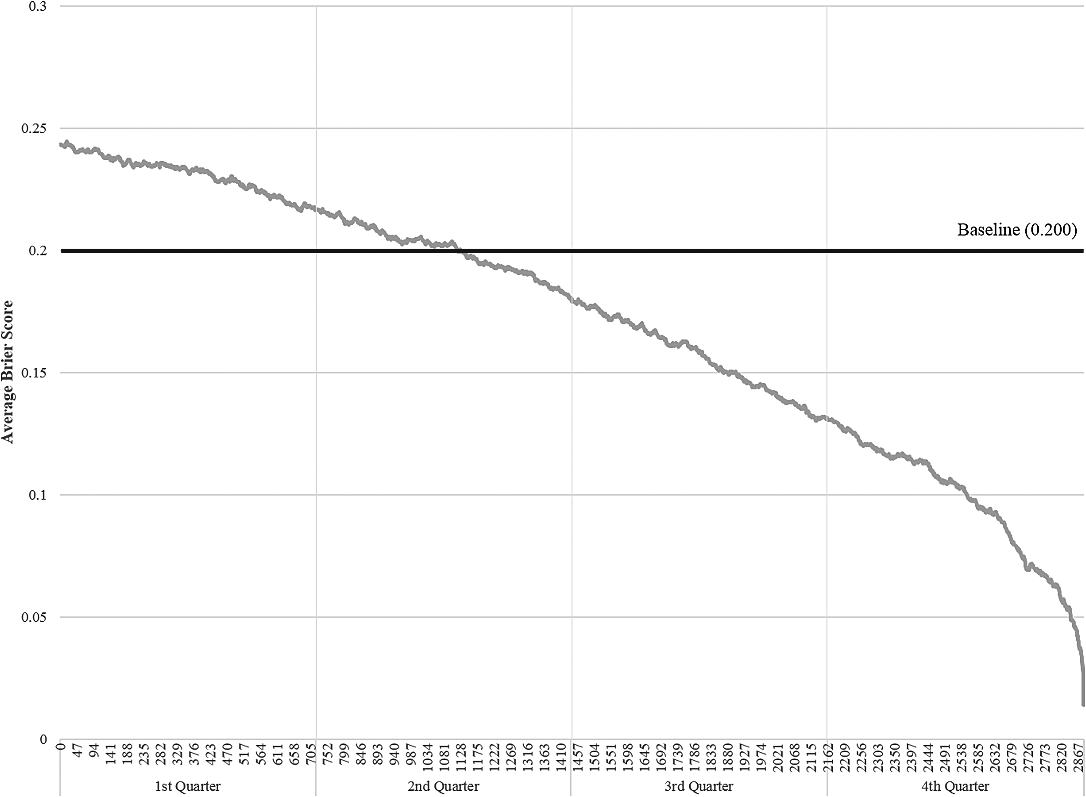
Average Brier score throughout a game.

Nearest neighbor analysis

Recall that the model relied on snapshots for which the Euclidean distance was 0 (i.e., exact match). That is, the model searched for snapshots in the training set that were the same as those obtained from the validation set. To see if we could improve the accuracy of the model, we incorporated the two nearest neighboring snapshots into the calculation in addition to the exact match. In this case, the algorithm found the exact match and the two closest point differences (one being higher and the other being lower than the exact point difference) at a given second. For example, if the home team had a 5-point lead at 5 minutes 0 seconds in the first quarter, the algorithm considered this snapshot along with a 4-point lead and 6-point lead (on their availability) at 5 minutes and 0 seconds to calculate the winning probabilities. Note that the nearest snapshots were identified by point difference but not time because we consider each second, S, a disparate state that is different than the preceding (S−1) and the following (S + 1) second in the game time line.

We also built a second version of this approach by changing the weights of the nearest neighbors. While the first version assigned equal weights to all three snapshots, the second version assigned 50% of the weight to the exact match and 25% of the weight to each nearest snapshot.

Both versions of the model generated the same results. The average Brier score was 0.170, with the highest being 0.721 and the lowest 0.008 (by both versions). The standard deviation was 0.133 (for both versions). These results were nearly the same as those obtained without the nearest neighbor approach. The model's accuracy was still below the baseline accuracy of 0.200.

As a test of robustness, we built models with more nearest neighbors. Specifically, we ran the same analysis by starting with the 2 nearest neighbors and then worked all the way up to the 10 nearest neighbors. In this case, the nearest neighbors were based on the proximity to the point difference observed in that second. For example, consider a 5-point lead at 5 minutes 0 seconds in the first quarter. If the algorithm considered the three nearest neighbors at this second of the game, all three could have been below 5 points (such as 4-, 3-, and 2-point leads) if the next nearest neighbor that was higher than the 5-point lead was a 9-point lead. As a result, we ran nine more analyses on the entire training set by changing the number of the nearest neighbors. The results were all the same: the mean Brier scores were 0.170.

Sensitivity analysis

Our training data set consisted of 23,532 games played in the past 20 seasons (from 1996–1997 to 2015–2016). This resulted in 68,398,501 snapshots, or rows of data, in our database. Therefore, the data analysis was resource intensive due to the amount of data that needed to be queried and processed. This also hinders the real-world use of the model. To see if we could achieve an acceptable value for the Brier score using a smaller training set, we conducted a sensitivity analysis and examined the change in the Brier score with respect to the size of the training set.

To this end, we split the training set into 20 subsets based on seasons so that each subset included the games of only one season. Then, we built new training sets in a cumulative manner using a reverse chronological order. For example, the first training set included only one season's games, which belonged to the most recent season (2015–2016). The second training set included the two most recent seasons' games (both 2015–2016 and 2014–2015). Therefore, the third training set included the three most recent seasons' games and so on. This resulted in 20 separate training sets, where the 20th set encompassed the entire training data used to test Model 1. Then, we ran Model 1 separately on each of these 20 training sets. This generated 20 separate analyses and thus 20 separate average Brier scores. We plotted the average Brier scores as a function of the training sets, presented in Figure 5. As seen in the figure, the training set that had only the most recent season's games (i.e., marked as 1 on the x-axis) generated an average Brier score of 0.176. The average Brier score improved to 0.171 if the data set included the games of only the last seven seasons (marked as 7 on the x-axis). As we added more seasons, the average Brier score improved, but the improvement was marginal: 20 seasons' data reduced the average Brier score to only 0.170.

FIG. 5.

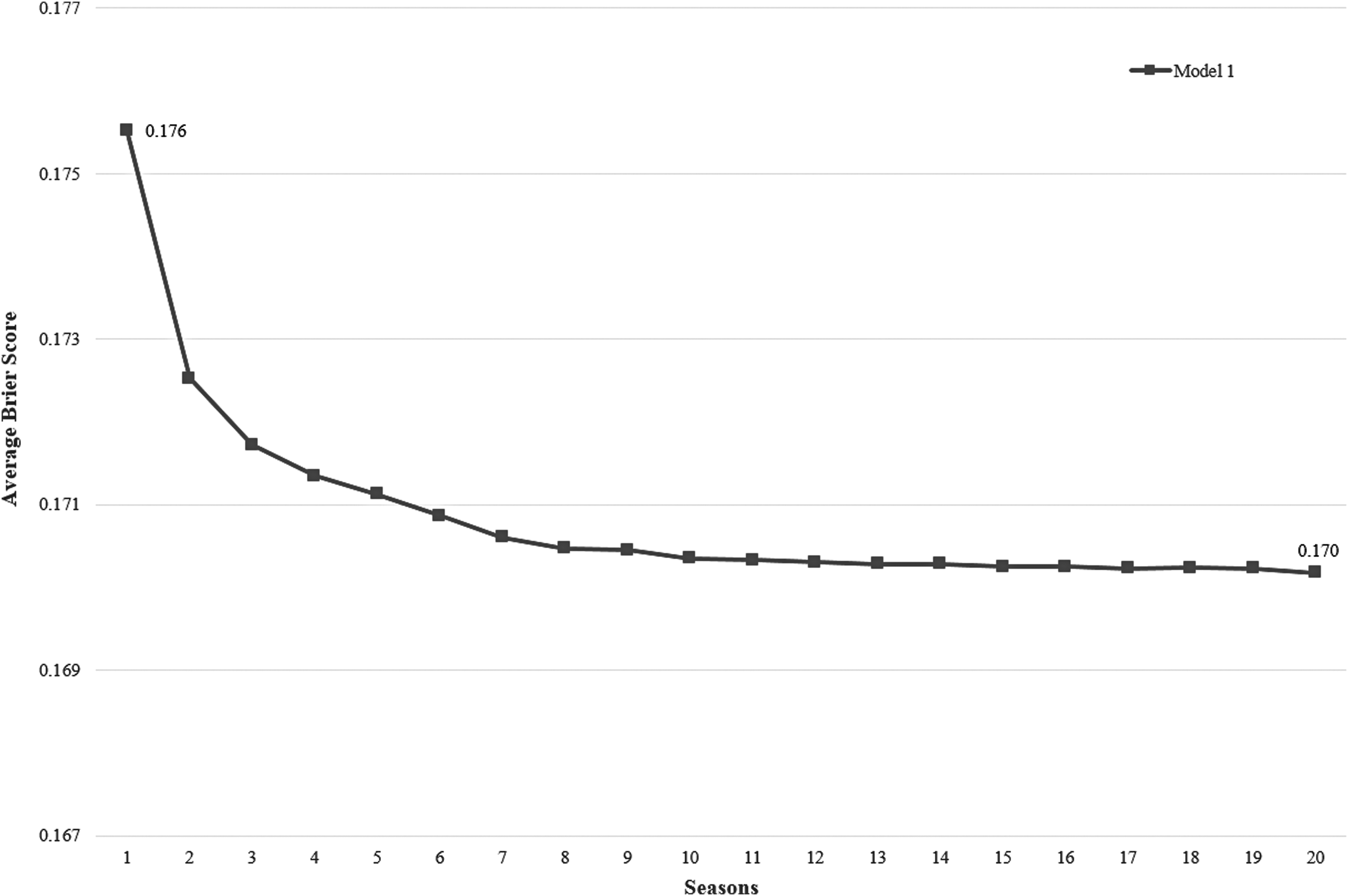
Sensitivity analysis of Model 1.

We also conducted a sensitivity analysis on the nearest neighbor approach. The results of the model that assigned equal weights to all three snapshots are presented in Figure 6. Note that the model that assigned 25% of the weight to each snapshot generated similar results; therefore, it is excluded. The results show that the nearest neighbor approach also performed better as the size of the training set increased. However, the nearest neighbor approach performed slightly better than the exact match approach when the training set used fewer seasons. For example, if the training set consisted only of the most current season's games (i.e., marked as 1 on the x-axis), the nearest neighbor approach generated an average Brier score of 0.172 while the same value was 0.176 for the exact match model. The difference becomes more apparent when there are three seasons' data (i.e., marked as 3 on the x-axis): the nearest neighbor approach achieves a Brier score of 0.171 with only three seasons' data, while the exact match needed seven seasons' data to achieve the same results.

FIG. 6.

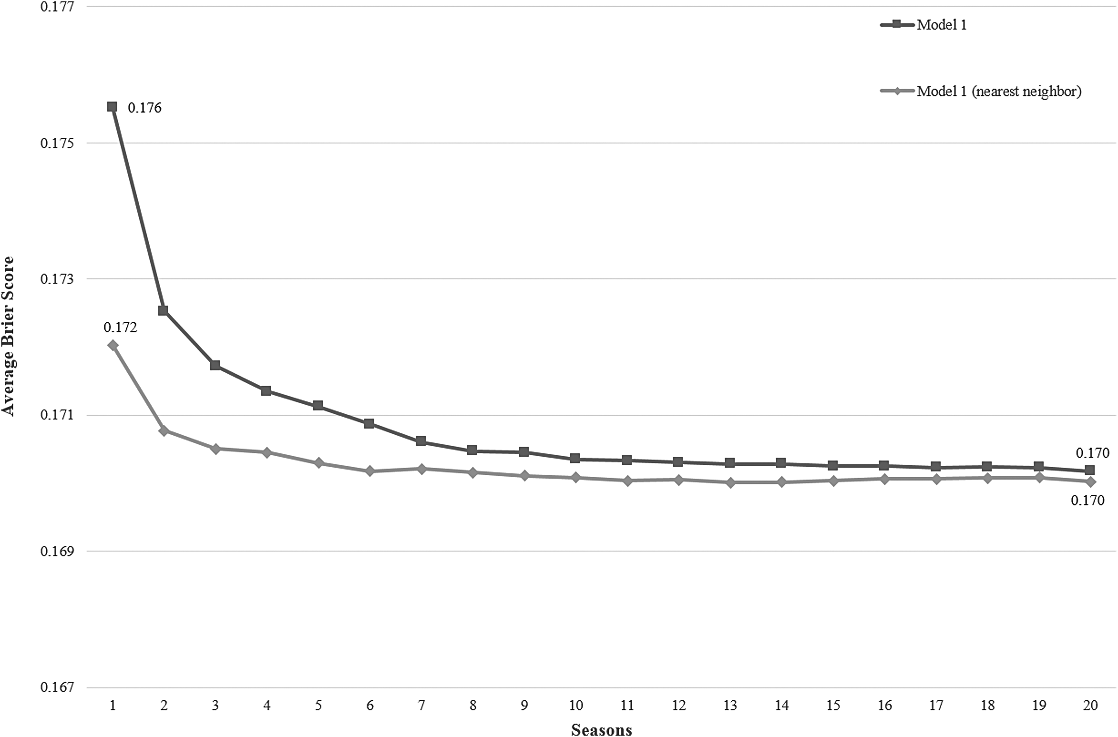
Sensitivity analysis of Model 1 with nearest neighbors.

Discussion

In Model 1, we used the point difference between the home and away teams as the only game attribute. Using this approach, we achieved an average Brier score of 0.170 when the training set included 20 seasons' data. This is well below the baseline accuracy of 0.200. Conducting a “leave-one-season-out” analysis generated similar—and in certain cases better—results, providing further validity for our findings. This also shows that Model 1 outperforms the predictions that are solely based on the in-game lead. The model makes timely predictions as well. The probabilities generated by the model improve as the game progresses, and the model starts converging on a winner by the middle of the second quarter.

Conducting a sensitivity analysis demonstrated that a training set that included only the last seven seasons' data achieved an average Brier score of 0.171. This shows that the training set can be drastically reduced to include only the most current seven seasons' data without compromising the accuracy of the model. This, in turn, increases the speed with which the algorithm runs and generates results.

Adopting a nearest neighbor approach did not significantly improve the model's accuracy. However, the nearest neighbor approach outperformed the exact match approach when the training set was smaller. This is expected because there are fewer exact matches in a smaller training set, and the nearest neighbor approach increases the number of available snapshots to calculate the probabilities of winning.

Model 2

In the second model, we focused on team strength in addition to the point difference. The rationale behind using team strength in the algorithm is self-evident: stronger teams should cling to their lead more firmly and thus have a higher probability of winning. For example, consider a team that has some of the best players in the league. A 10-point lead obtained by this team may not erode as easily as the same 10-point lead obtained by a weaker team. Therefore, this team may have a higher probability of winning than the other team, even if both teams enjoy the same point lead at a given time in the game.

To this end, we used the NBA's player impact estimate (PIE) metric as a proxy of team strength. The NBA defines PIE as “what % of game events did that player or team achieve.”¹³ The PIE score includes not only information about the points contributed by a player but also the player's other statistics, such as blocks, assists, steals, and rebounds. From this, the NBA also calculates a team's overall PIE score for each game and season. When aggregated at the team level, the PIE score provides information about the strength of a team and how it ranks compared with other teams. Overall, the NBA states that there is a strong correlation between a team's PIE score and its win record.¹³

Therefore, we used each team's end-of-season PIE score as that team's strength metric for that season. For instance, in the 2015–2016 season, we assigned the end-of-season PIE score of a team as that team's strength throughout all games played that season. We repeated this separately for all 20 seasons of games in our data set.

This approach provided us with two PIE scores for each game: one for the home team and one for the away team. To reconcile these PIE scores and determine which team had the advantage throughout a game, we took the difference to calculate the net PIE score for each game.

In this model, the algorithm used the point difference and net PIE score observed between the teams for each snapshot. Accordingly, it identified the point difference and the net PIE score between the home and away teams for each snapshot of each game in the validation set. Then, it identified all games in the training set that had the same point difference and same net PIE score. The outcomes of these games were used to calculate the winning probabilities of the teams. If the algorithm encountered unique snapshots in the validation set and could not find matching snapshots in the training set that had the same point difference and net PIE score, it searched for the nearest point differences and/or nearest PIE scores.

Results

Among the 1230 games in the validation set, the highest Brier score was 0.855 and the lowest was 0.002. The average Brier score of these games was 0.185 (with a standard deviation of 0.156). This was lower than the baseline accuracy (0.200). However, this model performed worse than Model 1. We tried different versions of Model 2 to handle the unique snapshots observed in the validation set. One of these searched for the closest net PIE score first and then the point difference, while the other searched for the closest point difference first and then the net PIE score. However, the results were essentially the same.

Nearest neighbor analysis

As is the case with Model 1, we built two more versions of this model to consider the two nearest snapshots in addition to the exact match. One of these used equal weights for all three snapshots, while the other used a weighted average (50% for the exact match and 25% for each of the nearest snapshots). Both models generated the same results. The average Brier score of the 1230 games was 0.182 (with a standard deviation of 0.155). The highest Brier score was 0.802 and the lowest one was 0.002. The average Brier score was lower than the baseline accuracy. Even though it was better than the exact match approach, the model was still worse than Model 1.

Sensitivity analysis

The data analysis took much longer due to the addition of the net PIE score in the algorithm. Therefore, we conducted a sensitivity analysis similar to the one conducted for Model 1 to see if accurate probabilities could be generated using a smaller training set.

The results, presented in Figure 7, show that both the exact match and the nearest neighbor versions of this model performed relatively worse than Model 1, regardless of the amount of data in the training set. Furthermore, the models performed particularly worse when the training data set was small and included only a few seasons worth of games.

FIG. 7.

Sensitivity analysis of Model 2.

Discussion

This model performed worse than Model 1. This shows that team strength, as conceptualized in this study, may not be as useful for predicting the in-game winning probabilities.

Furthermore, this model was more sensitive to the size of the training set than Model 1. As seen in Figure 7, this model performed poorly when the training set had only a few seasons' games. As the size of the training set increased, so did the accuracy of the model. However, the model still underperformed when compared with Model 1, even if the entire training set (i.e., 20 seasons' games) was used to generate the probabilities. This is because the model relies on two metrics to generate probabilities: the net PIE score and the point difference. This reduces the number of matching snapshots, which in turn results in poor predictions. For example, consider a game at the end of the first half (0 minutes 0 seconds of the second quarter), where the point difference between the teams is 0. Model 1 uses the outcomes of 918 games to generate the winning probabilities, whereas Model 2 uses only a subset of these 918 games by further filtering these games using the net PIE score. Therefore, if the net PIE score is 0 (which means the teams have equal strength), Model 2 uses the outcomes of only 63 games to generate probabilities. Even though this may generate better probabilities, reliance on fewer data points compromises the overall accuracy of the model. This did not improve, even if we created a nearest neighbor version of the model.

Note that one of the limitations of this analysis is that we used the end-of-season PIE scores as the strength of a team for that season. Instead, the analysis should have used a running PIE score for each team in each season that is calculated based on the games played by a team from the beginning of a season until each game day. However, we were not able to find or calculate these scores; therefore, we used the end-of-season PIE scores as a proxy.

Model 3

In this model, we replaced the team strength measure used in Model 2 with the rate of score change. We hypothesized that the rate by which a team generates a lead could increase the prediction accuracy when combined with the point difference observed between the teams. For example, a team that forces turnovers may score back-to-back goals without conceding any points. This, in turn, may increase the rate by which the point difference increases and can translate into a higher probability of winning for this team.

To this end, we needed to find the change in point difference between the home and away teams (Δ point difference) in a specific time frame (Δ time). We did not choose the time frame as 1 second because the rate of change in point difference within 1 second is already included in the point difference metric. Instead, we tried to identify a time frame within which a team fails to respond to the opposing team's potential goal and starts to fall behind.

Therefore, we used the NBA's PACE metric, which is defined as “the number of possessions per 48 minutes for a team or player.”¹³ In the 2015–2016 season, the average PACE value was 95.8, indicating that a team possessed the ball 95.8 times throughout a game.¹⁴ The average PACE value of the last 20 seasons is 91.7.¹⁴ This meant there were a total of 183.4 possessions (by both teams) on average in a typical NBA game throughout the 20 seasons used. Dividing 2880 seconds by 183.4 possessions shows that a team used a little more than 15 seconds per possession. This means that there is at least 30 seconds between the two goal attempts of the same team. Therefore, if there is a positive rate of change between 30 seconds, it means one of the teams squandered its possession and gave the advantage to the other team. For this reason, we decided to use a 30-second time interval to calculate the rate of score change. As a test of robustness, we also built two additional versions of this model based on a 15- and 60-second time interval.

Note that the rate of change is still stateless: it does not indicate which team has the lead. Consider the end of a game where a team has a 20-point lead. If this team starts missing goals in the last minute of the game and generates a negative rate of change, this may still not indicate the team's likelihood of losing the game due to this team's point advantage. Therefore, we used both the point difference and the rate of change in the algorithm.

To incorporate rate of change into the algorithm, we calculated the difference in point difference (Δ point difference) using a sliding 30-second window for each game in the training and validation sets. Due to the 30-second window, we were not able to calculate the rate of change for the first 30 seconds of each game. So the first 30 seconds of each game were excluded from this analysis.

Results

The model based on a 30-second interval generated the following results. Among the 1230 games in the validation set, the highest Brier score was 0.734 and the lowest was 0.012. The average Brier score of these games was 0.173 (with a standard deviation of 0.134). The average Brier score was lower than the baseline accuracy (0.200). Although this model outperformed Model 2, it performed worse than Model 1.

The models based on the 15- and the 60-second intervals generated similar findings. The average Brier score for the 15-second interval was 0.172, while the average Brier score for the 60-second interval was 0.174. Both values were lower than the baseline accuracy.

Nearest neighbor analysis

Like the earlier models, we built nearest neighbor versions of this model. However, we obtained the same results. For the 30-second interval model, the average Brier score was 0.172. As is the case with the earlier approaches, the model that assigned equal weights to each snapshot generated the same results as the model that used a weighted average for its nearest neighbors. The nearest neighbor approach generated the same results for the 15- and 60-second interval models as well. For these models, the average Brier score was between 0.172 and 0.174.

Sensitivity analysis

We conducted the same type of sensitivity analysis as for the earlier models. Note that we only discuss two of these analyses: (1) the 30-second interval model using an exact match and (2) the 30-second interval model using the nearest neighbor approach with equal weights. The results of the other analyses were nearly the same as these, so we excluded them. The results in Figure 8 show that both the exact match and the nearest neighbor models outperformed Model 2 but were still worse than Model 1.

FIG. 8.

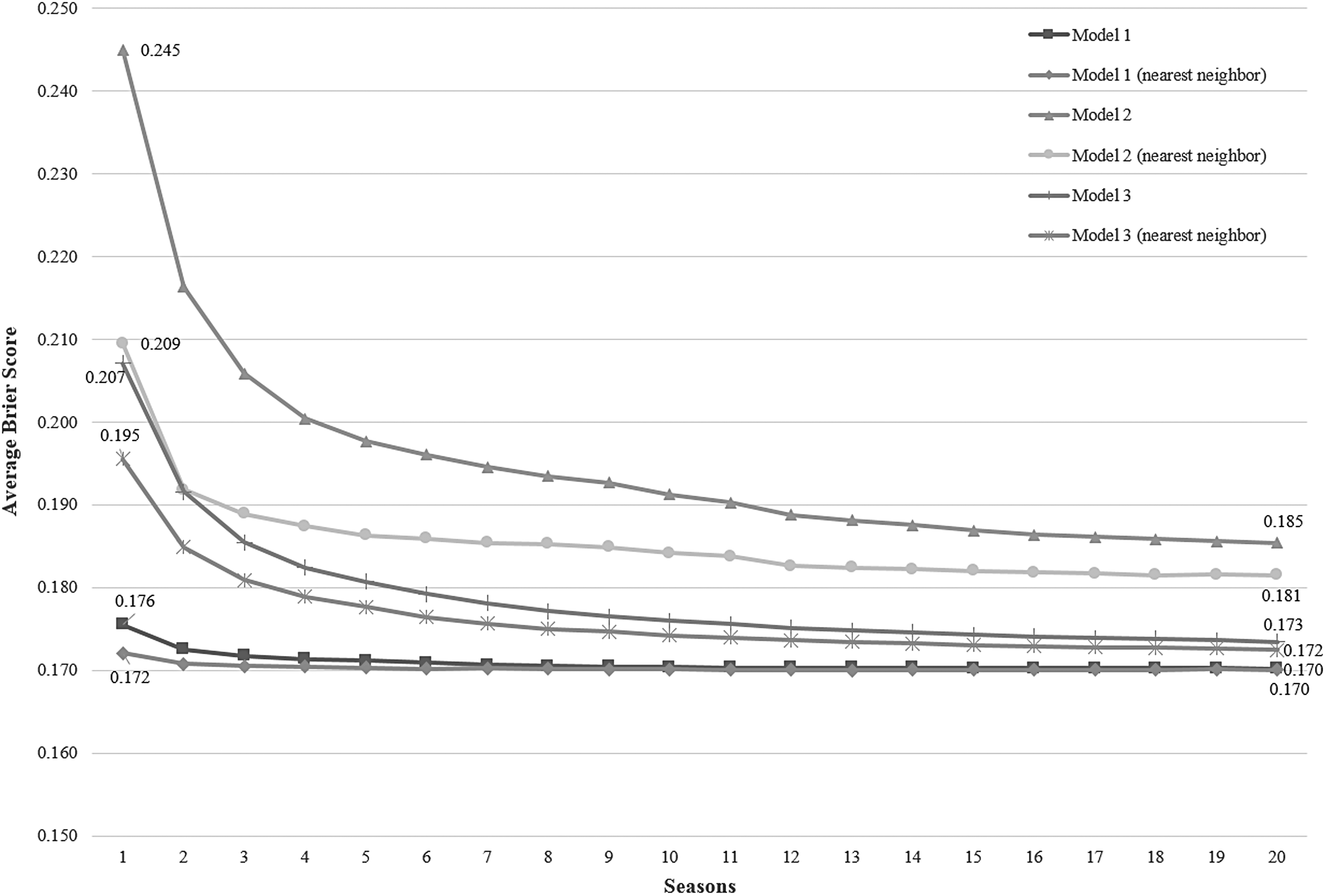
Sensitivity analysis of Model 3.

Discussion

This model made better predictions than Model 2, indicating that the rate of score change is a much better predictor of winning than team strength. However, the model still underperformed compared with Model 1.

This model suffered from the same pitfalls observed in Model 2: because the model used two metrics (the point difference and the rate of score change) to calculate the winning probabilities, it required more data to generate accurate predictions. As seen in Figure 8, the average Brier score starts to plateau much later than it does for Model 1. Even though the number of snapshots was increased by incorporating the two nearest snapshots into the algorithm, the model still could not perform as well as Model 1. Furthermore, as is the case with Model 2, having two metrics in each snapshot slowed down the algorithm significantly, making it less practical to use in a real-world setting.

General Discussion

Predicting the outcomes of sporting events has garnered the interest of many researchers, enthusiasts, and fans. Many different models have been proposed, ranging from unsophisticated comparisons to complex models. In this article, we proposed a novel approach that could calculate the in-game winning probabilities of NBA teams using a data snapshot approach. Our approach is different from earlier models in that we take a snapshot from the current game to capture essential in-game attributes and use the outcomes of historical games that have the same snapshot to make predictions about the winner of the current game.

Using this approach, we built three separate models. In Model 1, we used the point difference between the home and away teams as the only game attribute in each snapshot. In Model 2, we used the net PIE score (as a proxy for net team strength) in addition to the point difference in each snapshot. And in Model 3, we replaced the net PIE score used in Model 2 with the rate of score change. In addition to using the exact match approach, we also built the nearest neighbor versions of these models. The results are summarized in Table 1. Furthermore, Figure 9 shows the boxplots of the average Brier score generated by each model and compares them to the baseline accuracies discussed earlier.

FIG. 9.

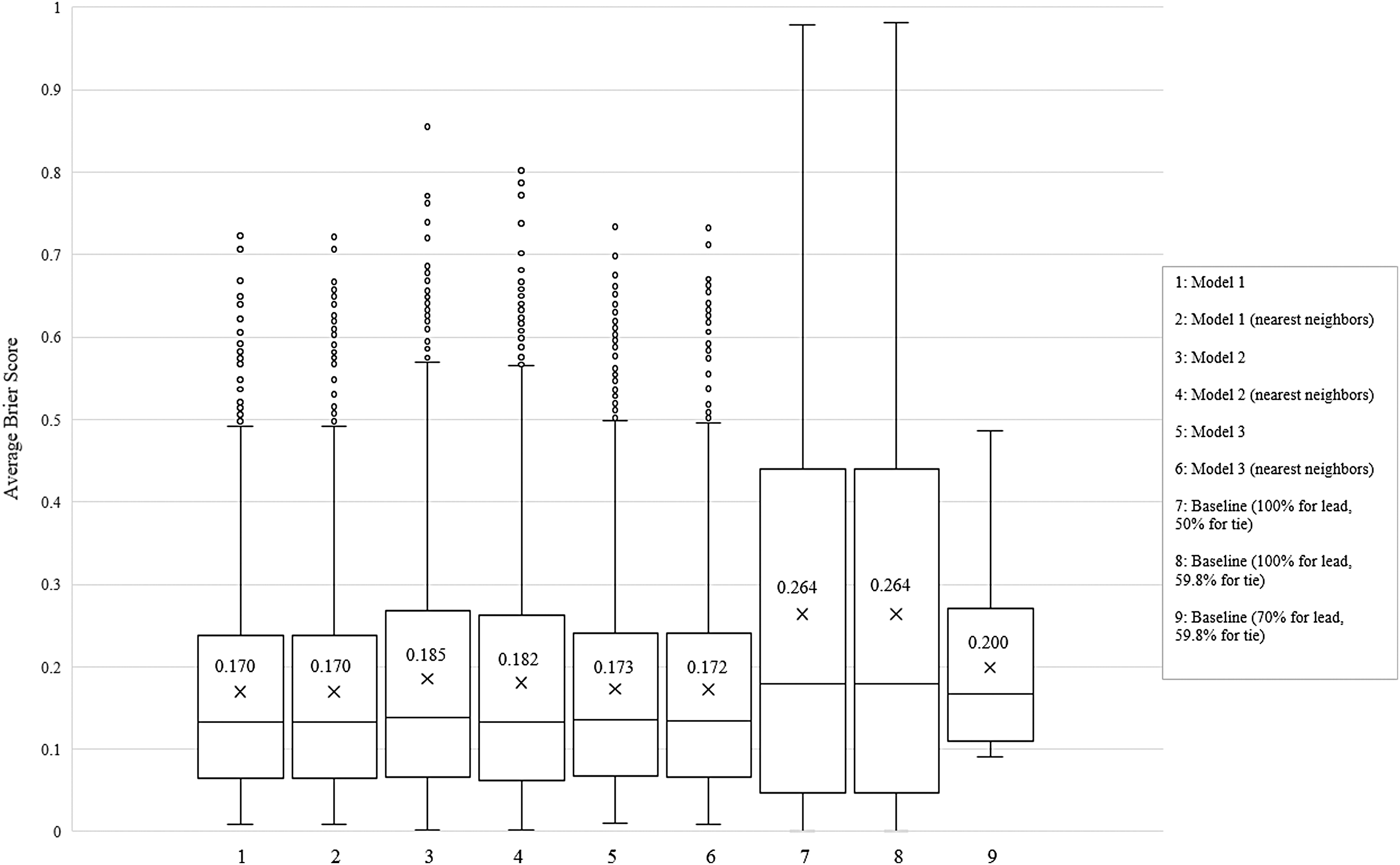
Boxplots of the models.

Table 1.

Summary of results

	Model 1 (exact match) ^a	Model 1 (nearest neighbor) ^a	Model 2 (exact match) ^a	Model 2 (nearest neighbor) ^a	Model 3 (exact match) ^a,b	Model 3 (nearest neighbor) ^a,b
Minimum Brier score	0.009	0.008	0.002	0.002	0.012	0.011
Maximum Brier score	0.722	0.721	0.855	0.820	0.734	0.734
Average Brier score	0.170	0.170	0.185	0.182	0.173	0.172

Results are based on the entire training data that include 20 seasons' games.

Rate of change is based on a 30-second interval.

The results of these analyses provide several important insights. First, the point difference between the home and away teams—as the only in-game attribute in each snapshot—not only generates accurate predictions but also requires much less data than the competing models. This increases the speed by which predictions are made because the amount of data that need to be searched is less than for Models 2 or 3. This also makes Model 1 the most practical to use in a real-world setting.

Second, the team strength—as conceptualized in this study—does not improve predictions. On the contrary, our conceptualization of team strength worsens the predictions. No matter how large the size of the training data, the model that uses team strength in addition to the point difference consistently underperforms and by a significant margin. Furthermore, the algorithm slows down because it tries to identify matching snapshots in the training set that satisfy both team strength and point difference requirements. This impedes the practicality of the algorithm.

Third, using the rate of score change in addition to the point difference in each snapshot results in marginally worse predictions, even though the predictions are still close to those generated by point difference alone. This also shows that rate of score change may not necessarily be a good predictor of winning. Furthermore, as in the case of team strength, the rate of score change requires a much larger data set to generate an acceptable level of accuracy. This impedes the real-world use of this algorithm as well.

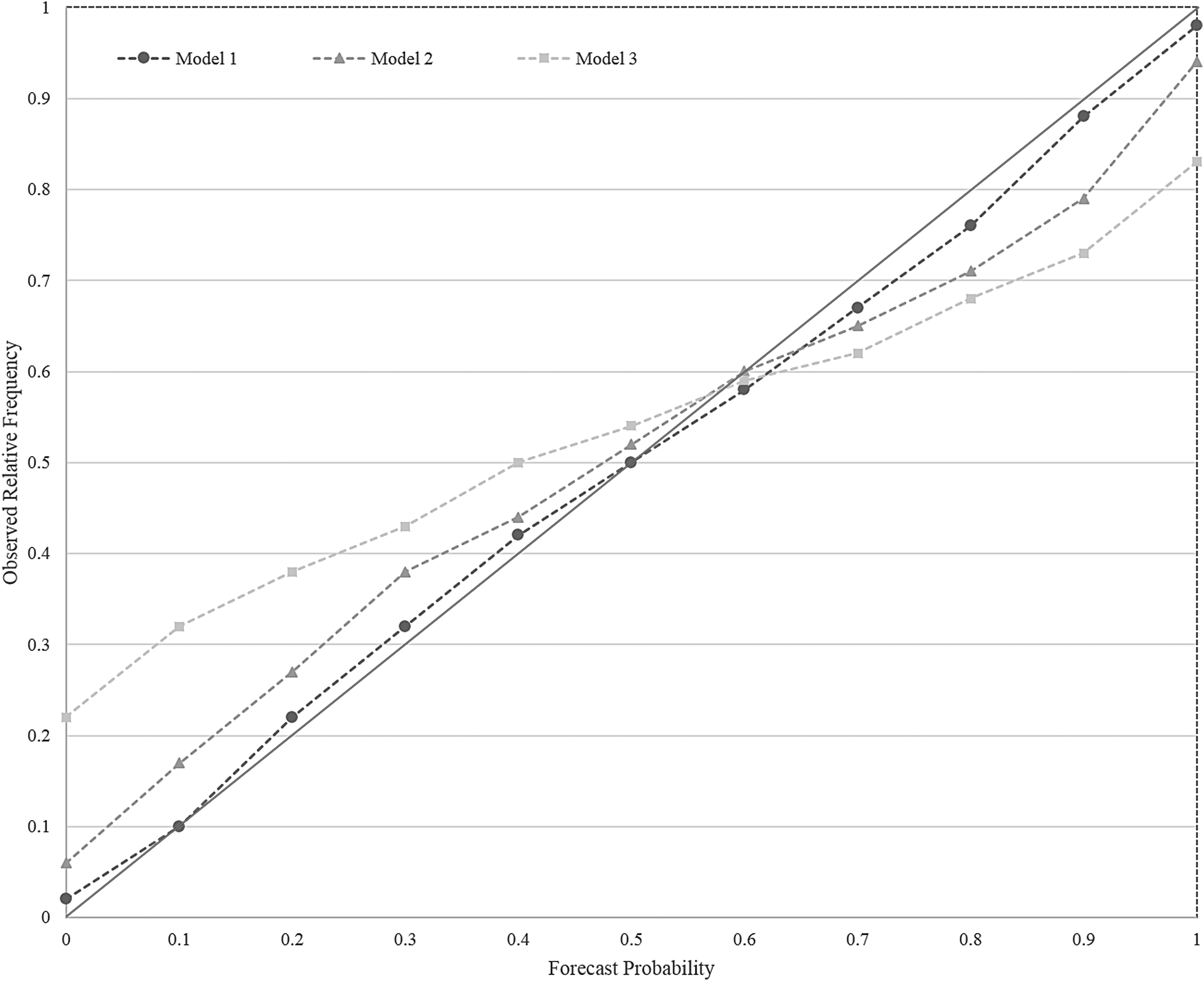
The reliability diagram, presented in Figure 10, further shows the validity of Model 1. This diagram, which compares the forecast probability to the observed relative frequency, helps evaluate models using the diagonal: the diagonal represents a perfect model.^15,16 Therefore, models closer to the diagonal are better than those that are farther away. As seen in the diagram, Model 1, which generates probability predictions using only the point difference, is very close to the diagonal. Note that the diagram does not include the nearest neighbor models because the reliability curves of these models coincided with the curves of their exact match models.

FIG. 10.

Reliability diagram.

The predictive ability of the point difference as the only in-game attribute deserves further discussion. Conventional wisdom suggests that the point difference is an overly simplistic predictor of in-game winning probabilities and that other metrics such as team strength should be included in the algorithm. This is because one may argue that a team's strength determines how well it can come back from a deficit or maintain a lead. However, it is important to note that strength may not always determine in-game performance. There could be other external factors, such as location, being on the road, or fatigue, that may influence a team's in-game performance. Therefore, it is possible for the strongest team to play like the weakest team or vice versa. An analysis of postgame interviews supports this because the losing side frequently indicates why the loss is not a true reflection of who they are, rather a deviation from their norm: “[we are] trying to figure out how we can get back to being ourselves”; “we obviously played one of our worst games”; “[I] didn't have it”; “I really just didn't have a rhythm”; “our energy was very low”; “[we] lost our spirit.”^17–23 Therefore, the point difference between the home and away teams is perhaps the best metric that can capture this unpredictable and ephemeral state that changes from one game to the next. Consequently, if the best player does not have a rhythm or if the players have low energy, even the best team plays like a weak team, which manifests itself in the point difference. In turn, this generates winning percentages in favor of the opposing team, regardless of the team's ranking or its players.

The approach proposed in this article can readily be applied to other sports because there is a growing interest in understanding the real-time or in-game winning probabilities of teams. For example, ESPN Analytics has a proprietary algorithm for football based on score, time remaining, field position, and down and distance.²⁴ Similarly, Pettigrew has an algorithm for hockey using time remaining and the home and away teams' goal-scoring rates.²⁵ There is no reason the snapshot approach proposed in this study cannot provide useful insights into these sports if the essential metrics can be captured in real time and compared with those observed in historical games.

Furthermore, the approach presented in this article can be applied in other contexts besides sports; it can be used wherever events unfold over a period of time during which there are observable metrics. For example, in the context of human resources, comparing an employee's weekly or monthly snapshots (for productivity, absence, citizenship, etc.) to those of previous employees' snapshots can identify at-risk employees in real time and help intervene before it is too late. Similarly, in the context of software development, comparing a project's snapshots (for lines of code, etc.) at specific time intervals with snapshots obtained from earlier projects can help predict the cost or delivery time. Or in the context of teaching, comparing a student's weekly snapshots (for quiz or assignment grades) with earlier students' snapshots can predict student success.

Conclusion

In this article, we proposed a data snapshot approach for generating the in-game winning probabilities of NBA teams. Using game data from the past 20 seasons, we compared the accuracies of three separate models. Our analyses showed that the point difference between the home and away teams at any given second of a game generates the best predictions and can use as little as seven seasons' data in the training set.

Footnotes

Author Disclosure Statement

No competing financial interests exist.

Cite this article as: Kayhan VO, Watkins A (2018) A data snapshot approach for making real-time predictions in basketball. Big Data 6:2, 96–112, DOI: 10.1089/big.2017.0054.

Abbreviations Used

References

Cooper

, DeNeve

, Mosteller

. Predicting professional sports game outcomes from intermediate game scores. Chance. 1992; 5:18–22.

McGivney

, McGivney

, Zegarelli

. Light It Up: Predicting the winner of an NBA game before the end. Chance. 2008; 21:45–50.

Stern

. A Brownian motion model for the progress of sports scores. J Am Stat Assoc. 1994; 89:1128–1134.

Gill

. Late-game reversals in professional basketball, football, and hockey. Am Stat. 2000; 54:94–99.

Shirley

. Markov model for basketball. In: New England Symposium for Statistics in Sports, Boston, MA, 2007.

Štrumbelj

, Vračar

. Simulating a basketball match with a homogeneous Markov model and forecasting the outcome. Int J Forecast. 2012; 28:532–542.

Vračar

, Štrumbelj

, Kononenko

. Modeling basketball play-by-play data. Expert Syst Appl. 2016; 44:58–66.

Martinez

. The influence of the first quarter on the final results in basketball. Revista Internacional de Medicina y Ciencias de la Actividad Fisica y del Deporte. 2014; 14:755–769.

Berger

, Pope

. Can losing lead to winning?. Manag Sci. 2011; 57:817–827.

10.

Ratanamahatana

, Keogh

. Making time-series classification more accurate using learned constraints. In: Proceedings of the 2004 SIAM International Conference on Data Mining, Lake Buena Vista, FL, 2004. pp. 11–22.

11.

Brier

. Verification of forecasts expressed in terms of probability. Mon Weather Rev. 1950; 78:1–3.

12.

Wilks

. Statistical methods in the atmospheric sciences. Boston, MA: Academic Press, 2011.

13.

NBA.com . Stat Glossary. Available online at http://stats.nba.com/help/glossary (last accessed June 8, 2017).

14.

Basketball-reference.com . NBA League Averages. Available online at www.basketball-reference.com/leagues/NBA_stats.html (last accessed June 8, 2017).

15.

Wilks

. On the combination of forecast probabilities for consecutive precipitation periods. Weather Forecast, 1990; 5:640–650.

16.

Murphy

, Winkler

. A general framework for forecast verification. Mon Weather Rev, 1987; 115:1330–1338.

17.

Moreno

. The Golden State Warriors Are Mortal, After All 2016. Available online at www.wxyz.com/newsy/the-golden-state-warriors-are-mortal-after-all (last accessed June 5, 2017).

18.

Wright

. Spurs hope to learn from squandered opportunity 2017. Available online at www.espn.com/blog/san-antonio-spurs/post/_/id/1514/spurs-hope-to-learn-from-squandered-opportunity (last accessed June 5, 2017).

19.

Forsberg

. Celtics' Gerald Green after loss: ‘We've been in this situation before’ 2017. Available online at www.espn.com/nba/story/_/id/19422624/after-blowout-loss-cleveland-cavaliers-game-2-boston-celtics-talk-moving-forward (last accessed June 5, 2017).

20.

MacMahon

. James Harden after romp, ouster: ‘Everything falls on my shoulders’ 2017. Available online at www.espn.com/nba/story/_/id/19362234/james-harden-houston-rockets-takes-responsibility-blames-rhythm (last accessed June 5, 2017).

21.

ESPN.com . Richard Jefferson: LeBron had a bug in Game 3 loss 2017. Available online at www.espn.com/nba/story/_/id/19452344/richard-jefferson-says-lebron-james-was-sick-cleveland-cavaliers-game-3-loss (last accessed June 5, 2017).

22.

McMenamin

. Tyronn Lue on uneven Cavs' loss to Hawks: ‘Games like this come back and bite you’ 2017. Available online at www.espn.com/nba/story/_/id/19107263/tyronn-lue-cavaliers-loss-hawks-games-come-back-bite-you (last accessed June 5, 2017).

23.

ESPN.com . Thursday's Clippers News: Rivers irked after loss to Timberwolves 2017. Available online at www.espn.com/blog/nba/post/_/id/30964/thursdays-clippers-news-rivers-irked-after-loss-to-timberwolves (last accessed June 5, 2017).

24.

ESPN Analytics. Charting the Patriots' incredible Super Bowl LI comeback 2017. Available online at www.espn.com/blog/statsinfo/post/_/id/128369/the-2016-nfl-playoffs-viewed-through-win-probability (last accessed June 5, 2017).

25.

Pettigrew

. Assessing the offensive productivity of NHL players using in-game win probabilities. Paper presented at the 9th Annual MIT Sloan Sports Analytics Conference, 2015.