Studies have shown that certain features from geography, demography, trade area, and environment can play a vital role in retail site selection, largely due to the impact they asserted on retail performance. Although the relevant features could be elicited by domain experts, determining the optimal feature set can be intractable and labor-intensive exercise. The challenges center around (1) how to determine features that are important to a particular retail business and (2) how to estimate retail sales performance given a new location? The challenges become apparent when the features vary across time. In this light, this study proposed a nonintervening approach by employing feature selection algorithms and subsequently sales prediction through similarity-based methods. The results of prediction were validated by domain experts. In this study, data sets from different sources were transformed and aggregated before an analytics data set that is ready for analysis purpose could be obtained. The data sets included data about feature location, population count, property type, education status, and monthly sales from 96 branches of a telecommunication company in Malaysia. The finding suggested that (1) optimal retail performance can only be achieved through fulfillment of specific location features together with the surrounding trade area characteristics and (2) similarity-based method can provide solution to retail sales prediction.
Introduction
Geospatial analytics can often be referred to as location analytics, spatial intelligence, and spatial analytics. It is commonly perceived as an intersection between business intelligence, geographic analysis, and data visualization. Geospatial analytics has not only gained importance commercially (e.g., Esri Maps, Foursquare, ShopperTrak), but it has also recently received attention academically. To date, geospatial analytics has been employed to tackle challenges in various domains including retail business,1 real estate, public safety,2 disaster monitoring and prevention, military exercises, government,2–4 planetary,5 agriculture,6–8 and renewal energy.9,10 Although the work presented in this article relaxed on the influence of customer behavior toward retail performance, it has focused on the implication of geospatial data on retail performance.
The importance of geospatial analytics to retail business can bring four benefits: (1) identify the optimal retail site for business expansion, (2) prediction of sales, (3) finding trade entities that coexist with a particular retail business, and (4) reallocation of existing outlets that are nonprofitable.
Store location and distribution intensity are important factors to store sales performance.11–17 A good site location is often the key to a store's success because it attracts consumers by offering them easy accessibility to products or services, which significantly influences market share and profitability. For many retailers and location theorists, the crucial criteria for opening a store is mainly the geographical information, traffic flow, accessibility to the area, competition, distance, cost, security of the region, local acceptance of the company, population density, and many more.3,12,18,19 Identifying the right features (variables) is not trivial because store performance is a function of such criteria.11,19 Store performance includes sales volume, store profits, market share, retail patronage, and price elasticity. Limited work has, however, been done to investigate the use of surrounding shops as indicator to site selection.20 Owing to the dynamics in business nature, retailers constantly monitor and project their sales to decide potential store reallocation.21 Careful retail trade area analyses were performed to analyze a potential location and estimated sales before opening a new store location.1
One common approach to site selection and sales prediction is through geographic information system (GIS). Such a visual inspection approach overlays different data sets, for example, population, traffic density, and geospatial information as the layers on a map and subsequently performs analysis on it. However, such an approach is nontrivial because active human involvement is required to perform exploratory analysis and extract hidden patterns from the layers. Such manual extraction of knowledge can be very labor intensive and often invites inaccurate interpretation due to overlapping of map layers. Rather than overlaying data set as different layers in a map, this research work flattens the layered data into structured analytics data set that fits analytics tasks. An analytics data set in this context refers to tabular data that aggregate different data sets from various sources to form a data frame that fits analytics exercises. The analytics data sets were then served as vehicle to answer the following objectives:
(1) To determine important variables for sales prediction given a particular retail business.
(2) To identify the optimal similarity measurement method for sales prediction of a new location.
In this study, five feature selection algorithms and four different similarity measurement methods were employed to obtain the optimal parameters for sales prediction given a location. The Related Work section proceeds with related work on site selection techniques whereas the Feature selection algorithms section highlights the importance of feature selection and the different algorithms that were used commonly by researchers. In the Method section, detailed algorithms proposed are discussed and are the main technical contributions by this work. Lastly, we discuss the impact of our study in the Results and Discussion before ending with the Conclusion.
Related Work
Retail site selection techniques
Various techniques have been employed by researchers to address challenges in retail trade area analysis.22 Among the most commonly employed techniques are the analog, regression, and gravity.23 An analog model relies on similar outlets' sales performances as reference to estimate the sales of potential new store locations. A regression model uses a number of independent features (variables), which are then used to predict the outcome of dependent feature (variable). In most cases, linear regression is employed to predict a sales value, whereas logistics regression is meant to predict the intensity of sales (i.e., high, moderate, and low). The third technique is the gravity model. Gravity models assert the assumption that customers within a specific radius of the retail store would have impact to its sales. That is, the bigger the radius, the insignificant the influence toward the store sales. Therefore, retail stores are often located nearer to the residential areas. One of the common gravity models is the Huff model.24 It is based on the principle that the probability of a given consumer visiting a given site is a function of the site distance, its attractiveness, together with the distance and attractiveness of the competing sites. However, the Huff model assumes homogeneity in consumers and lack of sensitivity to market segmentation. Therefore, more extensive perspectives must be considered when modeling a location selection problem not useful in specialized retailing.25
A recent study has reported that various critical errors occur during site selection.3 The flaws are (1) lack of study about the features and inappropriate use of the features for predictive model creation, (2) selection of a very remote place, (3) making decisions based on inadequate and insufficient samples, and (4) inadequate assessment of the competition. Among these features, using the correct features has been emphasis of many researches. Examples of variables used by researchers are road access,26 labor force,26,27 terrain,27 competition, climate, production cost,27 purchase capacity, and many more. Although various types of variables have been used, to date, no common practice and agreement on methods exist to elicit the variables.3 Often, human experts are required to handpick the features.28 The summary of various techniques used by researchers is given in Table 1.
TOPSIS, technique for order of preference by similarity to ideal solution.
Feature selection algorithms
Data set dimension reduction is an important process in data mining, aiming at improving model performance, measured by predictive accuracy, memory usage performance, and computational efficiency. In most domains, the dimension of data set is huge and often resorts to curse of dimensionality.29 To overcome such limitation, researchers have proposed dimensionality reduction approaches, namely, feature extraction and feature selection. Feature extraction is applied when the original high-dimensional feature space is projected into low-dimension feature space. Commonly used feature extraction methods are principal component analysis,30 linear discriminant analysis,31 and singular value decomposition.32 Another approach in reducing dimensionality of a data set is through feature selection. The ultimate goal is to identify a subset of features that could be used for model construction. Methods such as Lasso,33 Information Gain (IG),34 Relief,35 Fisher Score,36 and Laplacian Score37 have been widely reported in the literature.
With respect to search strategies, feature selection methods can be categorized into three groups. The first method is the filter approach.38–40 This is the preferable method because of its usability with different classifiers. The second method is the wrapper approach,41 which selects subsets of variables and assesses the fitness based on the classification accuracy. The third approach is the embedded method, which performs feature selection as part of the model construction process.42
Similarity-based method for prediction
There are a variety of studies for comparing similarity or distance measures in different domains and knowledge areas with regard to their own intention.43–46 However, the objective of the similarity or distance measures is the same in all contexts, which is to find the likeness or dissimilarity in the sets of points. For continuous data, Ref. 46 conducted a comparison study to investigate the behavior of low- and high-dimensional data with respect to the different similarity or distance measures. They compared and benchmarked 15 publicly available data sets with 12 distance measures such as Euclidean distance, average distance, chord distance, cosine measure, Mahalanobis distance, Manhattan distance, mean character difference, index of association, Canberra metric, Czekanowski coefficient, coefficient of divergence, and Pearson coefficient. The research gave an overall conclusion that the average distance is the most accurate and fastest distance measures among all the clustering algorithms. In contrast, for categorical data, Ref.47 carried out a comparison study on similarity measures and reviewed, compared, and benchmarked the categorical data based on binary-based similarity measures. For a specific knowledge area, for instance genetic interaction data sets, Ref.43 came to a conclusion that the dot product is consistent among the best measures in different circumstances. In another research, Ref.48 discussed four traditional distance measures, namely, Hausdorff distance, center of mass distance, link distance/earth movers distance and nearest-neighbor distance, and proposed two novel distances, that is, mutually-nearest distance and quad-tree distance to detect the geosocial similarity based on the locations of the users online activities. The study showed that the two novel distance measures were outperforming the existing distance measure in terms of accuracy and running time.
In this study, similarity-based methods were investigated with the aim to tackle the second and third challenges. In this work, four commonly practiced distance measure methods were considered, namely Euclidean distance, Manhattan distance, Hamming distance, and Gower distance.
Euclidean distance
The distance, \documentclass{aastex}\usepackage{amsbsy}\usepackage{amsfonts}\usepackage{amssymb}\usepackage{bm}\usepackage{mathrsfs}\usepackage{pifont}\usepackage{stmaryrd}\usepackage{textcomp}\usepackage{portland, xspace}\usepackage{amsmath, amsxtra}\usepackage{upgreek}\pagestyle{empty}\DeclareMathSizes{10}{9}{7}{6}\begin{document}
$$d ( x , y )$$
\end{document}, between two vectors x and y having p-dimensional space, is defined by
\documentclass{aastex}\usepackage{amsbsy}\usepackage{amsfonts}\usepackage{amssymb}\usepackage{bm}\usepackage{mathrsfs}\usepackage{pifont}\usepackage{stmaryrd}\usepackage{textcomp}\usepackage{portland, xspace}\usepackage{amsmath, amsxtra}\usepackage{upgreek}\pagestyle{empty}\DeclareMathSizes{10}{9}{7}{6}\begin{document}
\begin{align*}
d ( {\rm {\bf x} , {\bf y}} ) = \sum \limits_{i = 1}^p \sqrt {{{ ( {x_i} - {y_i} ) }^2}}. \tag{1}
\end{align*}
\end{document}
Euclidean is a special case of the Minkowski distance.49,50 Euclidean distance performs well when deployed to data sets that include compact or isolated clusters. This method can only be applied on numeric data. Therefore, in this work, only sales data were fed into this equation.
Manhattan distance
The distance is calculated as the sum of the absolute values of the differences between two observations. Unlike Euclidean, Manhattan only considers the horizontal and vertical distances. Manhattan distance is also known as Minowski distance.
\documentclass{aastex}\usepackage{amsbsy}\usepackage{amsfonts}\usepackage{amssymb}\usepackage{bm}\usepackage{mathrsfs}\usepackage{pifont}\usepackage{stmaryrd}\usepackage{textcomp}\usepackage{portland, xspace}\usepackage{amsmath, amsxtra}\usepackage{upgreek}\pagestyle{empty}\DeclareMathSizes{10}{9}{7}{6}\begin{document}
\begin{align*}
d ( {\rm {\bf x} , {\bf y}} ) = \sum \limits_{i = 1}^p \vert {x_i} - {y_i} \vert . \tag{2}
\end{align*}
\end{document}
Hamming distance
Such distance measure method has been widely used to calculate the distance between categorical variables. A contingency table is created to calculate the number of mismatches among the observations.
\documentclass{aastex}\usepackage{amsbsy}\usepackage{amsfonts}\usepackage{amssymb}\usepackage{bm}\usepackage{mathrsfs}\usepackage{pifont}\usepackage{stmaryrd}\usepackage{textcomp}\usepackage{portland, xspace}\usepackage{amsmath, amsxtra}\usepackage{upgreek}\pagestyle{empty}\DeclareMathSizes{10}{9}{7}{6}\begin{document}
\begin{align*}
d ( { \bf x } , { \bf y } ) = 1 - { \frac { \vert { \bf x } \cap { \bf y } \vert } { \vert { \bf x } \cup { \bf y } \vert } } . \tag { 3 }
\end{align*}
\end{document}
Gower distance
Gower distance is applied when the types of variables are a mixture of numeric and categorical variables. It computes the distance between the observations weighted by its variable type before taking the mean of the variables. The scaling of each variable to a [0, 1] is performed.51\documentclass{aastex}\usepackage{amsbsy}\usepackage{amsfonts}\usepackage{amssymb}\usepackage{bm}\usepackage{mathrsfs}\usepackage{pifont}\usepackage{stmaryrd}\usepackage{textcomp}\usepackage{portland, xspace}\usepackage{amsmath, amsxtra}\usepackage{upgreek}\pagestyle{empty}\DeclareMathSizes{10}{9}{7}{6}\begin{document}
\begin{align*}
d ( {\bf x} , {\bf y} ) = 1 - {S_{xy}} \tag{4}
\end{align*}
\end{document}\documentclass{aastex}\usepackage{amsbsy}\usepackage{amsfonts}\usepackage{amssymb}\usepackage{bm}\usepackage{mathrsfs}\usepackage{pifont}\usepackage{stmaryrd}\usepackage{textcomp}\usepackage{portland, xspace}\usepackage{amsmath, amsxtra}\usepackage{upgreek}\pagestyle{empty}\DeclareMathSizes{10}{9}{7}{6}\begin{document}
\begin{align*}
{ S_ { xy } } = { \frac { \sum \limits_ { k = 1 } ^p { w_ { xyk } } \, { s_ { xyk } } } { \sum \limits_ { k = 1 } ^p { w_ { xyk } } } } ,
\end{align*}
\end{document}
where \documentclass{aastex}\usepackage{amsbsy}\usepackage{amsfonts}\usepackage{amssymb}\usepackage{bm}\usepackage{mathrsfs}\usepackage{pifont}\usepackage{stmaryrd}\usepackage{textcomp}\usepackage{portland, xspace}\usepackage{amsmath, amsxtra}\usepackage{upgreek}\pagestyle{empty}\DeclareMathSizes{10}{9}{7}{6}\begin{document}
$${w_{xyk}}$$
\end{document} denotes the weight for variable k between observations x and y and \documentclass{aastex}\usepackage{amsbsy}\usepackage{amsfonts}\usepackage{amssymb}\usepackage{bm}\usepackage{mathrsfs}\usepackage{pifont}\usepackage{stmaryrd}\usepackage{textcomp}\usepackage{portland, xspace}\usepackage{amsmath, amsxtra}\usepackage{upgreek}\pagestyle{empty}\DeclareMathSizes{10}{9}{7}{6}\begin{document}
$${s_{xyk}}$$
\end{document} represents the distance between x and y on variable k.
The equation depicts a weighted average of the distances on the different variables. In Gower similarity index, \documentclass{aastex}\usepackage{amsbsy}\usepackage{amsfonts}\usepackage{amssymb}\usepackage{bm}\usepackage{mathrsfs}\usepackage{pifont}\usepackage{stmaryrd}\usepackage{textcomp}\usepackage{portland, xspace}\usepackage{amsmath, amsxtra}\usepackage{upgreek}\pagestyle{empty}\DeclareMathSizes{10}{9}{7}{6}\begin{document}
$${s_{xyk}}$$
\end{document} calculates the distance between x and y on variable k. In this study, the important variables were extracted through feature selection algorithms; therefore, the weight parameter in Gower equation carries the value “1.” The difference between Gower and other similarity measurements, \documentclass{aastex}\usepackage{amsbsy}\usepackage{amsfonts}\usepackage{amssymb}\usepackage{bm}\usepackage{mathrsfs}\usepackage{pifont}\usepackage{stmaryrd}\usepackage{textcomp}\usepackage{portland, xspace}\usepackage{amsmath, amsxtra}\usepackage{upgreek}\pagestyle{empty}\DeclareMathSizes{10}{9}{7}{6}\begin{document}
$${s_{xyk}}$$
\end{document}, does not apply the same calculation method to all the variables. The absolute difference is used for numeric variables, whereas for categorical variables, Gower uses equal comparison. To avoid bias on one type of variable having more impact on the distance metric, all \documentclass{aastex}\usepackage{amsbsy}\usepackage{amsfonts}\usepackage{amssymb}\usepackage{bm}\usepackage{mathrsfs}\usepackage{pifont}\usepackage{stmaryrd}\usepackage{textcomp}\usepackage{portland, xspace}\usepackage{amsmath, amsxtra}\usepackage{upgreek}\pagestyle{empty}\DeclareMathSizes{10}{9}{7}{6}\begin{document}
$${s_{xyk}}$$
\end{document} are scaled to the range [0, 1]. To be specific, \documentclass{aastex}\usepackage{amsbsy}\usepackage{amsfonts}\usepackage{amssymb}\usepackage{bm}\usepackage{mathrsfs}\usepackage{pifont}\usepackage{stmaryrd}\usepackage{textcomp}\usepackage{portland, xspace}\usepackage{amsmath, amsxtra}\usepackage{upgreek}\pagestyle{empty}\DeclareMathSizes{10}{9}{7}{6}\begin{document}
$${s_{xyk}}$$
\end{document} will be assigned “0” when the categorical variables of x and y are equal and “1” when they are not.
\documentclass{aastex}\usepackage{amsbsy}\usepackage{amsfonts}\usepackage{amssymb}\usepackage{bm}\usepackage{mathrsfs}\usepackage{pifont}\usepackage{stmaryrd}\usepackage{textcomp}\usepackage{portland, xspace}\usepackage{amsmath, amsxtra}\usepackage{upgreek}\pagestyle{empty}\DeclareMathSizes{10}{9}{7}{6}\begin{document}
\begin{align*}
{s_{xyk}} = \left( { \begin{matrix} {0 , } & {{ \rm{if}} \ {X_{xk}} = {X_{yk}}} \\ {1 , } & {{ \rm{if}} \ {X_{xk}} \ne {X_{yk}}}. \\ \end{matrix} } \right.
\end{align*}
\end{document}
As for numeric variables, they are scaled by dividing the absolute difference by the range of the variable.
\documentclass{aastex}\usepackage{amsbsy}\usepackage{amsfonts}\usepackage{amssymb}\usepackage{bm}\usepackage{mathrsfs}\usepackage{pifont}\usepackage{stmaryrd}\usepackage{textcomp}\usepackage{portland, xspace}\usepackage{amsmath, amsxtra}\usepackage{upgreek}\pagestyle{empty}\DeclareMathSizes{10}{9}{7}{6}\begin{document}
\begin{align*}
{ s_ { xyk } } = { \frac { \vert { X_ { xk } } - { X_ { yk } } \vert } { max ( { X_k } ) - min ( { X_k } ) } } ,
\end{align*}
\end{document}
where \documentclass{aastex}\usepackage{amsbsy}\usepackage{amsfonts}\usepackage{amssymb}\usepackage{bm}\usepackage{mathrsfs}\usepackage{pifont}\usepackage{stmaryrd}\usepackage{textcomp}\usepackage{portland, xspace}\usepackage{amsmath, amsxtra}\usepackage{upgreek}\pagestyle{empty}\DeclareMathSizes{10}{9}{7}{6}\begin{document}
$${X_{xk}}$$
\end{document} denotes the value of variable k for object x.
Method
This section discusses the source and structure of raw data sets used in this study. The raw data sets were transformed into an analytics data set before subsequent analytics tasks were performed.
Table 2 presents the six data sets, with partial feature list shown, used in this study. Let \documentclass{aastex}\usepackage{amsbsy}\usepackage{amsfonts}\usepackage{amssymb}\usepackage{bm}\usepackage{mathrsfs}\usepackage{pifont}\usepackage{stmaryrd}\usepackage{textcomp}\usepackage{portland, xspace}\usepackage{amsmath, amsxtra}\usepackage{upgreek}\pagestyle{empty}\DeclareMathSizes{10}{9}{7}{6}\begin{document}
$${{ \cal D}_{poi}}$$
\end{document} denote the points of interest data set, which consists of 418,324 places of interest (e.g., shop, schools, and shopping malls) in Malaysia. The places of interest are categorized into 1232 categories. Examples of column names are business name, address, business type, latitude, longitude, and description. The data set was obtained from Telekom Malaysia and is updated half-yearly. The second data set is the Malaysian population data set (\documentclass{aastex}\usepackage{amsbsy}\usepackage{amsfonts}\usepackage{amssymb}\usepackage{bm}\usepackage{mathrsfs}\usepackage{pifont}\usepackage{stmaryrd}\usepackage{textcomp}\usepackage{portland, xspace}\usepackage{amsmath, amsxtra}\usepackage{upgreek}\pagestyle{empty}\DeclareMathSizes{10}{9}{7}{6}\begin{document}
$${{ \cal D}_{pop}}$$
\end{document}), which was obtained from the Department of Statistics Malaysia (DOSM). The data set contains population information about different races at both district and subdistrict level. \documentclass{aastex}\usepackage{amsbsy}\usepackage{amsfonts}\usepackage{amssymb}\usepackage{bm}\usepackage{mathrsfs}\usepackage{pifont}\usepackage{stmaryrd}\usepackage{textcomp}\usepackage{portland, xspace}\usepackage{amsmath, amsxtra}\usepackage{upgreek}\pagestyle{empty}\DeclareMathSizes{10}{9}{7}{6}\begin{document}
$${{ \cal D}_{job}}$$
\end{document} stores information about different job types for all the districts in Malaysia, whereas \documentclass{aastex}\usepackage{amsbsy}\usepackage{amsfonts}\usepackage{amssymb}\usepackage{bm}\usepackage{mathrsfs}\usepackage{pifont}\usepackage{stmaryrd}\usepackage{textcomp}\usepackage{portland, xspace}\usepackage{amsmath, amsxtra}\usepackage{upgreek}\pagestyle{empty}\DeclareMathSizes{10}{9}{7}{6}\begin{document}
$${{ \cal D}_{edu}}$$
\end{document} presents the different educational levels, ranging from O'Level to bachelor degree. Both the data sets were also provided by Telekom Malaysia. \documentclass{aastex}\usepackage{amsbsy}\usepackage{amsfonts}\usepackage{amssymb}\usepackage{bm}\usepackage{mathrsfs}\usepackage{pifont}\usepackage{stmaryrd}\usepackage{textcomp}\usepackage{portland, xspace}\usepackage{amsmath, amsxtra}\usepackage{upgreek}\pagestyle{empty}\DeclareMathSizes{10}{9}{7}{6}\begin{document}
$${{ \cal D}_{ppt}}$$
\end{document} consists of data about different property types at street level for the whole Malaysia. Examples of property type captured in the data set are terrace, apartment, single story, and bungalow. This data set was contributed by a property company in Malaysia. \documentclass{aastex}\usepackage{amsbsy}\usepackage{amsfonts}\usepackage{amssymb}\usepackage{bm}\usepackage{mathrsfs}\usepackage{pifont}\usepackage{stmaryrd}\usepackage{textcomp}\usepackage{portland, xspace}\usepackage{amsmath, amsxtra}\usepackage{upgreek}\pagestyle{empty}\DeclareMathSizes{10}{9}{7}{6}\begin{document}
$${{ \cal D}_{ppt}}$$
\end{document} was provided by a property company in Malaysia. The last data set used in this study is the company sales data set (\documentclass{aastex}\usepackage{amsbsy}\usepackage{amsfonts}\usepackage{amssymb}\usepackage{bm}\usepackage{mathrsfs}\usepackage{pifont}\usepackage{stmaryrd}\usepackage{textcomp}\usepackage{portland, xspace}\usepackage{amsmath, amsxtra}\usepackage{upgreek}\pagestyle{empty}\DeclareMathSizes{10}{9}{7}{6}\begin{document}
$${{ \cal D}_{telcoSales}}$$
\end{document}). It consists of monthly sales for the year 2016 and for every branch of that telecommunication company in Malaysia. The monthly sales were aggregated into yearly sales. All the data sets provided by the respective authorities had gone through thorough screening to remove all customer level information.
UPSR, Ujian Pencapaian Sekolah Rendah (Primary School Evaluation Test); PMR, Penilaian Menengah Rendah (Lower Certificate of Education); SPM, Sijil Pelajaran Malaysia (Malaysian Certificate of Education); STPM, Sijil Tinggi Persekolahan Malaysia (Higher School Certificate).
Transforming raw to analytics data set
The process of transforming the raw data sets into an analytics data set can be accomplished with three proposed algorithms. Transformation is required because analytics data set is a prerequisite to subsequent analytics tasks, namely, feature selection and sales prediction.
Algorithm 1 shows the high-level process of constructing the analytics data set required for this study. The algorithm takes in six raw data sets as input, whereas the output is the transformed analytics data set. Based on Algorithm 1, the first step is extracting the latitudes and longitudes of all the 96 locations from the \documentclass{aastex}\usepackage{amsbsy}\usepackage{amsfonts}\usepackage{amssymb}\usepackage{bm}\usepackage{mathrsfs}\usepackage{pifont}\usepackage{stmaryrd}\usepackage{textcomp}\usepackage{portland, xspace}\usepackage{amsmath, amsxtra}\usepackage{upgreek}\pagestyle{empty}\DeclareMathSizes{10}{9}{7}{6}\begin{document}
$${{ \cal D}_{telcoSales}}$$
\end{document} data set; the results are stored as \documentclass{aastex}\usepackage{amsbsy}\usepackage{amsfonts}\usepackage{amssymb}\usepackage{bm}\usepackage{mathrsfs}\usepackage{pifont}\usepackage{stmaryrd}\usepackage{textcomp}\usepackage{portland, xspace}\usepackage{amsmath, amsxtra}\usepackage{upgreek}\pagestyle{empty}\DeclareMathSizes{10}{9}{7}{6}\begin{document}
$${ \mathcal{L}_{96}}$$
\end{document}. From \documentclass{aastex}\usepackage{amsbsy}\usepackage{amsfonts}\usepackage{amssymb}\usepackage{bm}\usepackage{mathrsfs}\usepackage{pifont}\usepackage{stmaryrd}\usepackage{textcomp}\usepackage{portland, xspace}\usepackage{amsmath, amsxtra}\usepackage{upgreek}\pagestyle{empty}\DeclareMathSizes{10}{9}{7}{6}\begin{document}
$${{ \cal D}_{telcoSales}}$$
\end{document}, monthly sales are then extracted and stored as \documentclass{aastex}\usepackage{amsbsy}\usepackage{amsfonts}\usepackage{amssymb}\usepackage{bm}\usepackage{mathrsfs}\usepackage{pifont}\usepackage{stmaryrd}\usepackage{textcomp}\usepackage{portland, xspace}\usepackage{amsmath, amsxtra}\usepackage{upgreek}\pagestyle{empty}\DeclareMathSizes{10}{9}{7}{6}\begin{document}
$${{ \cal D}_{sales ( 96 ) }}$$
\end{document}. The next process is the construction of \documentclass{aastex}\usepackage{amsbsy}\usepackage{amsfonts}\usepackage{amssymb}\usepackage{bm}\usepackage{mathrsfs}\usepackage{pifont}\usepackage{stmaryrd}\usepackage{textcomp}\usepackage{portland, xspace}\usepackage{amsmath, amsxtra}\usepackage{upgreek}\pagestyle{empty}\DeclareMathSizes{10}{9}{7}{6}\begin{document}
$${{ \cal D}_{loc ( 96 ) }}$$
\end{document} data set. This is done through the generate site-FeatureMatrix function, where surrounding shops from each of the 96 locations are extracted and structured in the form of a database table. generate site-FeatureMatrix searched through the \documentclass{aastex}\usepackage{amsbsy}\usepackage{amsfonts}\usepackage{amssymb}\usepackage{bm}\usepackage{mathrsfs}\usepackage{pifont}\usepackage{stmaryrd}\usepackage{textcomp}\usepackage{portland, xspace}\usepackage{amsmath, amsxtra}\usepackage{upgreek}\pagestyle{empty}\DeclareMathSizes{10}{9}{7}{6}\begin{document}
$${ \mathcal{L}_{96}}$$
\end{document} and extracted all the shops within \documentclass{aastex}\usepackage{amsbsy}\usepackage{amsfonts}\usepackage{amssymb}\usepackage{bm}\usepackage{mathrsfs}\usepackage{pifont}\usepackage{stmaryrd}\usepackage{textcomp}\usepackage{portland, xspace}\usepackage{amsmath, amsxtra}\usepackage{upgreek}\pagestyle{empty}\DeclareMathSizes{10}{9}{7}{6}\begin{document}
$$100m$$
\end{document} of the 96 points. From all the location characteristics extracted, a table will be formed that records the loca tion features of a business. The table consists of 96 rows that represent the location features of each outlet. Algorithm 1 proceeds with extraction of all the relevant data from \documentclass{aastex}\usepackage{amsbsy}\usepackage{amsfonts}\usepackage{amssymb}\usepackage{bm}\usepackage{mathrsfs}\usepackage{pifont}\usepackage{stmaryrd}\usepackage{textcomp}\usepackage{portland, xspace}\usepackage{amsmath, amsxtra}\usepackage{upgreek}\pagestyle{empty}\DeclareMathSizes{10}{9}{7}{6}\begin{document}
$${{ \cal D}_{pop}}$$
\end{document}, \documentclass{aastex}\usepackage{amsbsy}\usepackage{amsfonts}\usepackage{amssymb}\usepackage{bm}\usepackage{mathrsfs}\usepackage{pifont}\usepackage{stmaryrd}\usepackage{textcomp}\usepackage{portland, xspace}\usepackage{amsmath, amsxtra}\usepackage{upgreek}\pagestyle{empty}\DeclareMathSizes{10}{9}{7}{6}\begin{document}
$${{ \cal D}_{poi}}$$
\end{document}, \documentclass{aastex}\usepackage{amsbsy}\usepackage{amsfonts}\usepackage{amssymb}\usepackage{bm}\usepackage{mathrsfs}\usepackage{pifont}\usepackage{stmaryrd}\usepackage{textcomp}\usepackage{portland, xspace}\usepackage{amsmath, amsxtra}\usepackage{upgreek}\pagestyle{empty}\DeclareMathSizes{10}{9}{7}{6}\begin{document}
$${{ \cal D}_{job}}$$
\end{document}, \documentclass{aastex}\usepackage{amsbsy}\usepackage{amsfonts}\usepackage{amssymb}\usepackage{bm}\usepackage{mathrsfs}\usepackage{pifont}\usepackage{stmaryrd}\usepackage{textcomp}\usepackage{portland, xspace}\usepackage{amsmath, amsxtra}\usepackage{upgreek}\pagestyle{empty}\DeclareMathSizes{10}{9}{7}{6}\begin{document}
$${{ \cal D}_{ppt}}$$
\end{document}, \documentclass{aastex}\usepackage{amsbsy}\usepackage{amsfonts}\usepackage{amssymb}\usepackage{bm}\usepackage{mathrsfs}\usepackage{pifont}\usepackage{stmaryrd}\usepackage{textcomp}\usepackage{portland, xspace}\usepackage{amsmath, amsxtra}\usepackage{upgreek}\pagestyle{empty}\DeclareMathSizes{10}{9}{7}{6}\begin{document}
$${{ \cal D}_{edu}}$$
\end{document} through the extract-Data function. In this work, rather than perceiving the six data sets as different layers on a map as presented in the conventional GIS approach, the data sets were transformed into an analytics data set by performing a relational algebra named natural join on them.
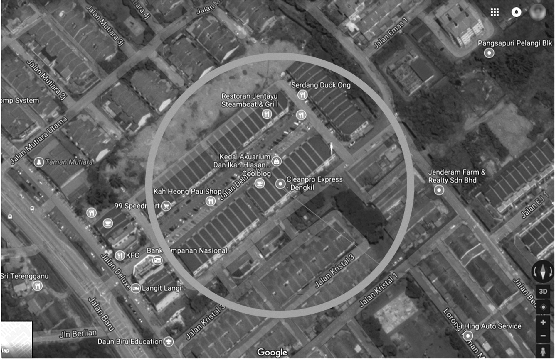
The generate site-FeatureMatrix function takes in point of interest data set (\documentclass{aastex}\usepackage{amsbsy}\usepackage{amsfonts}\usepackage{amssymb}\usepackage{bm}\usepackage{mathrsfs}\usepackage{pifont}\usepackage{stmaryrd}\usepackage{textcomp}\usepackage{portland, xspace}\usepackage{amsmath, amsxtra}\usepackage{upgreek}\pagestyle{empty}\DeclareMathSizes{10}{9}{7}{6}\begin{document}
$${{ \cal D}_{poi}}$$
\end{document}) and the 96 locations (\documentclass{aastex}\usepackage{amsbsy}\usepackage{amsfonts}\usepackage{amssymb}\usepackage{bm}\usepackage{mathrsfs}\usepackage{pifont}\usepackage{stmaryrd}\usepackage{textcomp}\usepackage{portland, xspace}\usepackage{amsmath, amsxtra}\usepackage{upgreek}\pagestyle{empty}\DeclareMathSizes{10}{9}{7}{6}\begin{document}
$${{ \cal D}_{96}}$$
\end{document}) as input while returning \documentclass{aastex}\usepackage{amsbsy}\usepackage{amsfonts}\usepackage{amssymb}\usepackage{bm}\usepackage{mathrsfs}\usepackage{pifont}\usepackage{stmaryrd}\usepackage{textcomp}\usepackage{portland, xspace}\usepackage{amsmath, amsxtra}\usepackage{upgreek}\pagestyle{empty}\DeclareMathSizes{10}{9}{7}{6}\begin{document}
$${{ \cal D}_{poi ( 96 ) }}$$
\end{document} as an output. The function begins with extracting shops within 100 m distance from each company branch for all the 96 branches. The extraction process has shown that the number of shops within 100 m distance from a company branch can range from 50 to 100, depending on the design of the trade areas. For instance in Figure 1, taking Cleanpro Express–Dengkil as point of interest, the number of shops within 100 m is 51. From the list of shops, \documentclass{aastex}\usepackage{amsbsy}\usepackage{amsfonts}\usepackage{amssymb}\usepackage{bm}\usepackage{mathrsfs}\usepackage{pifont}\usepackage{stmaryrd}\usepackage{textcomp}\usepackage{portland, xspace}\usepackage{amsmath, amsxtra}\usepackage{upgreek}\pagestyle{empty}\DeclareMathSizes{10}{9}{7}{6}\begin{document}
$${{ \cal P}_{all}}$$
\end{document}, only the unique shops are filtered and subsequently sorted descending according to its frequency. In this study, only 15 shops with highest frequencies were then served as input to the Site-FeatureMatrix function to generate \documentclass{aastex}\usepackage{amsbsy}\usepackage{amsfonts}\usepackage{amssymb}\usepackage{bm}\usepackage{mathrsfs}\usepackage{pifont}\usepackage{stmaryrd}\usepackage{textcomp}\usepackage{portland, xspace}\usepackage{amsmath, amsxtra}\usepackage{upgreek}\pagestyle{empty}\DeclareMathSizes{10}{9}{7}{6}\begin{document}
$${{ \cal D}_{poi ( 96 ) }}$$
\end{document}. In \documentclass{aastex}\usepackage{amsbsy}\usepackage{amsfonts}\usepackage{amssymb}\usepackage{bm}\usepackage{mathrsfs}\usepackage{pifont}\usepackage{stmaryrd}\usepackage{textcomp}\usepackage{portland, xspace}\usepackage{amsmath, amsxtra}\usepackage{upgreek}\pagestyle{empty}\DeclareMathSizes{10}{9}{7}{6}\begin{document}
$${{ \cal D}_{poi ( 96 ) }}$$
\end{document}, each row i \documentclass{aastex}\usepackage{amsbsy}\usepackage{amsfonts}\usepackage{amssymb}\usepackage{bm}\usepackage{mathrsfs}\usepackage{pifont}\usepackage{stmaryrd}\usepackage{textcomp}\usepackage{portland, xspace}\usepackage{amsmath, amsxtra}\usepackage{upgreek}\pagestyle{empty}\DeclareMathSizes{10}{9}{7}{6}\begin{document}
$$\in$$
\end{document} {1, 96} represents a company branch, whereas the columns j\documentclass{aastex}\usepackage{amsbsy}\usepackage{amsfonts}\usepackage{amssymb}\usepackage{bm}\usepackage{mathrsfs}\usepackage{pifont}\usepackage{stmaryrd}\usepackage{textcomp}\usepackage{portland, xspace}\usepackage{amsmath, amsxtra}\usepackage{upgreek}\pagestyle{empty}\DeclareMathSizes{10}{9}{7}{6}\begin{document}
$$\in$$
\end{document} {1, 20} represent the 20 location features. The cell ij stores the weight of the row i in the context of column j and the weight w\documentclass{aastex}\usepackage{amsbsy}\usepackage{amsfonts}\usepackage{amssymb}\usepackage{bm}\usepackage{mathrsfs}\usepackage{pifont}\usepackage{stmaryrd}\usepackage{textcomp}\usepackage{portland, xspace}\usepackage{amsmath, amsxtra}\usepackage{upgreek}\pagestyle{empty}\DeclareMathSizes{10}{9}{7}{6}\begin{document}
$$\in$$
\end{document} {TRUE, FALSE}. That is, a cell with TRUE implies that for that particular branch i, there exists a shop j within 100 m distance.
1: for\documentclass{aastex}\usepackage{amsbsy}\usepackage{amsfonts}\usepackage{amssymb}\usepackage{bm}\usepackage{mathrsfs}\usepackage{pifont}\usepackage{stmaryrd}\usepackage{textcomp}\usepackage{portland, xspace}\usepackage{amsmath, amsxtra}\usepackage{upgreek}\pagestyle{empty}\DeclareMathSizes{10}{9}{7}{6}\begin{document}
$$i = 1$$
\end{document} to 96 do
2: if town-match(\documentclass{aastex}\usepackage{amsbsy}\usepackage{amsfonts}\usepackage{amssymb}\usepackage{bm}\usepackage{mathrsfs}\usepackage{pifont}\usepackage{stmaryrd}\usepackage{textcomp}\usepackage{portland, xspace}\usepackage{amsmath, amsxtra}\usepackage{upgreek}\pagestyle{empty}\DeclareMathSizes{10}{9}{7}{6}\begin{document}
$${ \mathcal{L}_{96}} [ i ]$$
\end{document},\documentclass{aastex}\usepackage{amsbsy}\usepackage{amsfonts}\usepackage{amssymb}\usepackage{bm}\usepackage{mathrsfs}\usepackage{pifont}\usepackage{stmaryrd}\usepackage{textcomp}\usepackage{portland, xspace}\usepackage{amsmath, amsxtra}\usepackage{upgreek}\pagestyle{empty}\DeclareMathSizes{10}{9}{7}{6}\begin{document}
$${{ \cal D}_d}$$
\end{document}) then
3: extract town level data for d
4: else if subdistrict-match(\documentclass{aastex}\usepackage{amsbsy}\usepackage{amsfonts}\usepackage{amssymb}\usepackage{bm}\usepackage{mathrsfs}\usepackage{pifont}\usepackage{stmaryrd}\usepackage{textcomp}\usepackage{portland, xspace}\usepackage{amsmath, amsxtra}\usepackage{upgreek}\pagestyle{empty}\DeclareMathSizes{10}{9}{7}{6}\begin{document}
$${ \mathcal{L}_{96}} [ i ]$$
\end{document},\documentclass{aastex}\usepackage{amsbsy}\usepackage{amsfonts}\usepackage{amssymb}\usepackage{bm}\usepackage{mathrsfs}\usepackage{pifont}\usepackage{stmaryrd}\usepackage{textcomp}\usepackage{portland, xspace}\usepackage{amsmath, amsxtra}\usepackage{upgreek}\pagestyle{empty}\DeclareMathSizes{10}{9}{7}{6}\begin{document}
$${{ \cal D}_d}$$
\end{document}) then
5: extract subdistrict level data for d
6: else if district-match(\documentclass{aastex}\usepackage{amsbsy}\usepackage{amsfonts}\usepackage{amssymb}\usepackage{bm}\usepackage{mathrsfs}\usepackage{pifont}\usepackage{stmaryrd}\usepackage{textcomp}\usepackage{portland, xspace}\usepackage{amsmath, amsxtra}\usepackage{upgreek}\pagestyle{empty}\DeclareMathSizes{10}{9}{7}{6}\begin{document}
$${ \mathcal{L}_{96}} [ i ]$$
\end{document},\documentclass{aastex}\usepackage{amsbsy}\usepackage{amsfonts}\usepackage{amssymb}\usepackage{bm}\usepackage{mathrsfs}\usepackage{pifont}\usepackage{stmaryrd}\usepackage{textcomp}\usepackage{portland, xspace}\usepackage{amsmath, amsxtra}\usepackage{upgreek}\pagestyle{empty}\DeclareMathSizes{10}{9}{7}{6}\begin{document}
$${{ \cal D}_d}$$
\end{document}) then
7: extract district level for d
8: end if
9: end for
The extract-Data function is called in line no. 5 in Algorithm 1. The function takes in two parameters, namely \documentclass{aastex}\usepackage{amsbsy}\usepackage{amsfonts}\usepackage{amssymb}\usepackage{bm}\usepackage{mathrsfs}\usepackage{pifont}\usepackage{stmaryrd}\usepackage{textcomp}\usepackage{portland, xspace}\usepackage{amsmath, amsxtra}\usepackage{upgreek}\pagestyle{empty}\DeclareMathSizes{10}{9}{7}{6}\begin{document}
$${{ \cal D}_d}$$
\end{document} and \documentclass{aastex}\usepackage{amsbsy}\usepackage{amsfonts}\usepackage{amssymb}\usepackage{bm}\usepackage{mathrsfs}\usepackage{pifont}\usepackage{stmaryrd}\usepackage{textcomp}\usepackage{portland, xspace}\usepackage{amsmath, amsxtra}\usepackage{upgreek}\pagestyle{empty}\DeclareMathSizes{10}{9}{7}{6}\begin{document}
$${ \mathcal{L}_{96}}$$
\end{document}. Let \documentclass{aastex}\usepackage{amsbsy}\usepackage{amsfonts}\usepackage{amssymb}\usepackage{bm}\usepackage{mathrsfs}\usepackage{pifont}\usepackage{stmaryrd}\usepackage{textcomp}\usepackage{portland, xspace}\usepackage{amsmath, amsxtra}\usepackage{upgreek}\pagestyle{empty}\DeclareMathSizes{10}{9}{7}{6}\begin{document}
$${ \mathcal{L}_{96}}$$
\end{document} denote the 96 branches, whereas \documentclass{aastex}\usepackage{amsbsy}\usepackage{amsfonts}\usepackage{amssymb}\usepackage{bm}\usepackage{mathrsfs}\usepackage{pifont}\usepackage{stmaryrd}\usepackage{textcomp}\usepackage{portland, xspace}\usepackage{amsmath, amsxtra}\usepackage{upgreek}\pagestyle{empty}\DeclareMathSizes{10}{9}{7}{6}\begin{document}
$${{ \cal D}_d}$$
\end{document} denotes the five data sets used in this study with d\documentclass{aastex}\usepackage{amsbsy}\usepackage{amsfonts}\usepackage{amssymb}\usepackage{bm}\usepackage{mathrsfs}\usepackage{pifont}\usepackage{stmaryrd}\usepackage{textcomp}\usepackage{portland, xspace}\usepackage{amsmath, amsxtra}\usepackage{upgreek}\pagestyle{empty}\DeclareMathSizes{10}{9}{7}{6}\begin{document}
$$\in \{ poi , pop , edu , job , ppt \} $$
\end{document}. For each location \documentclass{aastex}\usepackage{amsbsy}\usepackage{amsfonts}\usepackage{amssymb}\usepackage{bm}\usepackage{mathrsfs}\usepackage{pifont}\usepackage{stmaryrd}\usepackage{textcomp}\usepackage{portland, xspace}\usepackage{amsmath, amsxtra}\usepackage{upgreek}\pagestyle{empty}\DeclareMathSizes{10}{9}{7}{6}\begin{document}
$${ \mathcal{L}_{96}} [ i ]$$
\end{document}, the function extracts relevant data at different granularity from the data set. The function will first attempt to match relevant data at town level. This is mainly because town level provides data localized to the branch and could better reflect the actual scenario. In addition, having data at the lower granularity often elicits better prediction outcomes. If no town-level data can be acquired, the function will then proceed to matching of subdistrict-level data. The last alternative is to use the data at the district level.
10: \documentclass{aastex}\usepackage{amsbsy}\usepackage{amsfonts}\usepackage{amssymb}\usepackage{bm}\usepackage{mathrsfs}\usepackage{pifont}\usepackage{stmaryrd}\usepackage{textcomp}\usepackage{portland, xspace}\usepackage{amsmath, amsxtra}\usepackage{upgreek}\pagestyle{empty}\DeclareMathSizes{10}{9}{7}{6}\begin{document}
$$ { { \cal S } _e } \leftarrow \frac { 1 } { 5 } { { \cal D } _ { sales ( \mathcal { L } _ { min ( SS { T_ { d , fs } } ) } ^5 ) } } $$
\end{document}
11: end for
The mentioned algorithm shows the process for estimating sales for a given new location. The input to the algorithm is the sales for 96 outlets, whereas the output is the Sum-of-Square values and predicted sales for a given new location. The algorithm begins with ranking descendingly the entire data set according to sales. This allows creation of three clusters using the threshold 33% and 67% cut. The mean sales for each cluster are calculated. The next process is two for-loops. The iterative process first identifies five existing locations with shortest distance from the new location. The calculation of distance takes into consideration different feature selection methods and distance measurement techniques. The lowest \documentclass{aastex}\usepackage{amsbsy}\usepackage{amsfonts}\usepackage{amssymb}\usepackage{bm}\usepackage{mathrsfs}\usepackage{pifont}\usepackage{stmaryrd}\usepackage{textcomp}\usepackage{portland, xspace}\usepackage{amsmath, amsxtra}\usepackage{upgreek}\pagestyle{empty}\DeclareMathSizes{10}{9}{7}{6}\begin{document}
$$SS{T_{d , fs}}$$
\end{document} denotes the most similar location characteristics with the given location and, therefore, allows the relevant five locations to be identified for calculation of sales.
Results and Discussion
In this research work, the algorithms were implemented and executed using R programming language.52 R has existing software packages that can be modified to fit this research work.
As discussed in the Method section, raw data sets were transformed into an analytics data set before feature selection and sales prediction can be performed. The transformed data set, however, consisted of a huge set of features. As shown in Table 3, there are 103 features in total and, therefore, reducing the large feature space was the first analytics task in this study.
Analytics data set
NType of features
Count
Point of interest
20
Population
6
Job
34
Education
22
Property
20
Sales
1
Total
103
Findings on feature selection
Five feature selection algorithms were employed in this study, namely, Boruta,53Recursive Feature Elimination (RFE),54Feature Subset Computation (FSC),55Random Forest (RF),56 and IG.57 Boruta is a feature selection algorithm that works as wrapper around RF. Boruta follows an all-relevant feature selection method wherein it finds all the variables that are relevant to the dependent variable. The relevant R package is Boruta. The next feature selection algorithm employed is FSC. It is based on wrapper method to reduce features and can be implemented using the RoughSets package. The third feature selection algorithm is RFE. It follows the wrapper approach with greedy optimization algorithm aiming at finding the best performing subset of features. It repeatedly constructs a model and setting the best or worst features aside and iterates the process until all the features in the data set are exhausted. The relevant R package is caret.
There were two filter-based feature selection algorithms employed in this study. They are RF and IG. In RF, the importance of each variable was calculated using mean decrease accuracy, with the aim to determine the impact of each feature on the models accuracy. RF can be implemented through the R package named FSelector. The last feature selection algorithm employed is IG. It is used to assign a scoring to each feature. The score indicates the importance of each feature. The subset of features can be selected based on the absolute number of features with highest importance, a certain percentage of features with highest importance, and whose importance exceeds a certain threshold value. IG can be performed through the mlr package in R.
Table 4 shows two categories of features elicited by five feature selection algorithms. In this study, experiments were constrained to only top 20 features from each feature selection algorithm. Coincidentally, FSC identified only 21 features from 103 variables and, therefore, all the 21 features were considered in the experiments. From the table, most algorithms elicited more numeric variables except for the FSC algorithm. IG has the most numerical variables, whereas FSC selected the least as compared with others. Conversely, FSC selected the most categorical variables, whereas IG identified only 1 out of 20 variables. The detail of variables selected by each feature selection algorithm is shown in Tables 5 and 6. In Table 5, shopping shop, four story shop house, and four story shop are among the categorical variables popular among the feature selection algorithms. As for numerical features, human health and social work activities, low secondary education, water supply sewerage waste management and recovery, arts entertainment and recreation, family workers without salary, and education are among the top features selected by most feature selection algorithms.
Categories of features by feature selection algorithms
Feature selection algorithm
No. of numeric variables
No. of categorical variables
Total no. of features
Boruta
16
4
20
RFE
13
7
20
FSC
6
15
21
RF
15
5
20
IG
19
1
20
FSC, feature subset computation; IG, information gain; RF, random forest; RFE, recursive feature elimination.
Categorical variables by feature selection algorithms
Features
Boruta
RFE
FSC
RF
IG
Shopping shop
x
x
x
x
Four story shop house
x
x
x
Low cost house
x
x
x
x
Four story shop
x
x
x
x
Post office
x
x
Travel agency
x
x
Apartments
x
TM point
x
Chinese food restaurant
x
Building
x
Private clinic
x
Private clinic PM care
x
Kurnia agents
x
Detached house
x
One story shop
x
Semidetached house
x
Two story shop house
x
Three story shop house
x
Five story shop
x
PM, privatized management; TM, Telekom Malaysia.
Numerical variables by different feature selection algorithms
Features
Boruta
RFE
FSC
RF
IG
Human health and social work activities
x
x
x
x
Low secondary education
x
x
x
x
Water supply sewerage waste management and recovery
x
x
x
x
Education
x
x
x
x
UPSR
x
x
x
Public administration and defense
x
x
x
PMR
x
x
x
Diploma in polytechnic
x
x
x
Advanced diploma
x
Arts entertainment and recreation
x
x
x
x
Transport and storage
x
x
Not in school
x
x
x
Household activity
x
Skilled worker and carpenters
x
x
x
Family workers without salary
x
x
x
x
STPM
x
x
x
Mining and quarrying
x
x
Chinese
x
x
Bachelor
x
Preuniversity
x
Other Bumiputera
x
Financial and insurance
x
Real estate activities
x
Manufacturing
x
Certificate of polytechnic university
x
Manager
x
Still in school
x
Graduated
x
Never go to school
x
High secondary education
x
Diploma
x
No certificate
x
SPM
x
Advanced diploma
x
Tables 7 and 8 show the sources of the selected features. The tables indicated that most of the features originated from the job category. This category comprises features used to describe the type of business by the local people. Examples of features in the job category are family workers without salary, household activity, transportation, and storage and many more. The two tables also show that education is the second factor contributed to the list of selected features. The experiment findings indicated that location features were not as many as other categories of variables. The findings also showed that population did not play much role in the sales prediction. This is largely because the data provided by DOSM is a higher level, that is at district or subdistrict levels. Therefore, population in the context can be negligible.
Feature selected by wrapper approach
Feature selection
Variable
category
Features
Count
Boruta
Location
Shopping shop
1
Property
Four story shop house, low cost house, four story shop
3
Job
Human health and social work activities, water supply sewerage waste management and recovery, education, public administration and defense, arts entertainment and recreation, transport and storage, household activity, skilled worker and carpenters, family workers without salary
9
Education
Low secondary education, UPSR, PMR, diploma in polytechnic, advanced diploma, not in school, STPM
7
Population
—
0
RFE
Location
Shopping shop, post office, travel agency
3
Property
Four story shop house, low cost house, four story shop, apartments
4
Job
Human health and social work activities, water supply sewerage waste management and recovery, mining and quarrying, education, family workers without salary, arts entertainment and recreation, public administration and defense, transport and storage
TM point, Chinese food restaurant, building, private clinic, shopping shop, private clinic PM care, Kurnia agents, travel agency,
8
Property
Detached house, One story shop, semidetached house, four story shop, two story shop house, three story shop house, five story shop,
7
Job
Water supply sewerage waste management and recovery activities, financial and insurance, real estate activities, family workers without salary
4
Education
—
0
Population
Other Bumiputera, Chinese
2
Feature selected by filter approach
Feature selection
Variable category
Features
Count
RF
Location
Shopping shop, post office,
2
Property
Four story shop house, certificate of polytechnic university, low cost house, four story shop
4
Job
Human health and social work activities. Water supply sewerage waste management and recovery, education, skilled worker and carpenters, mining and quarrying, arts entertainment and recreation, manufacturing, manager
8
Education
Low secondary education, PMR, UPSR, STPM, diploma in polytechnic, not in school
6
Population
—
0
IG
Location
—
0
Property
Low cost house,
1
Job
Skilled worker and carpenters, public administration and defense, education, human health and social work activities, arts entertainment and recreation, family workers without salary,
6
Education
Still in school, graduated, not in school, never go to school, low secondary education, high secondary education, diploma, no certificate, UPSR, PMR, SPM, diploma in polytechnic, advanced diploma
13
Population
—
0
Evaluation for distance measurement
The results given in Table 9 are sum of squares (SST) for each location with respect to five feature selection algorithms and distance measurement techniques. SST is the sum of squares of the difference between the response variable (sales) and its mean, \documentclass{aastex}\usepackage{amsbsy}\usepackage{amsfonts}\usepackage{amssymb}\usepackage{bm}\usepackage{mathrsfs}\usepackage{pifont}\usepackage{stmaryrd}\usepackage{textcomp}\usepackage{portland, xspace}\usepackage{amsmath, amsxtra}\usepackage{upgreek}\pagestyle{empty}\DeclareMathSizes{10}{9}{7}{6}\begin{document}
$${ \bar c_i}$$
\end{document}. It is used to measure the variation in the response variable. The SST values were calculated based on the normalized sales data. Referring to Algorithm 4 line no. 8, SST value can be calculated using the following formula:
\documentclass{aastex}\usepackage{amsbsy}\usepackage{amsfonts}\usepackage{amssymb}\usepackage{bm}\usepackage{mathrsfs}\usepackage{pifont}\usepackage{stmaryrd}\usepackage{textcomp}\usepackage{portland, xspace}\usepackage{amsmath, amsxtra}\usepackage{upgreek}\pagestyle{empty}\DeclareMathSizes{10}{9}{7}{6}\begin{document}
\begin{align*}
SS{T_{d , fs}} = \sum \limits_{i = 1}^5 { ( {{ \cal D}_{{sales} ( \mathcal{L}_{d , fs}^i ) }} - { \bar c_i} ) ^2}.
\end{align*}
\end{document}
Total sum of square for four different locations
Feature selection
Location
Euclidean
Manhattan
Jaccard
Gower
BORUTA
1
0.2484
0.1231
0.7605
0.2454
2
0.5785
0.2369
0.4825
0.6171
3
0.3316
0.8522
0.7605
0.8164
4
0.3269
0.3413
0.1792
0.2821
Average for Boruta
0.3713
0.3884
0.5456
0.4902
RFE
1
0.1285
0.1542
0.4135
0.4732
2
0.5709
0.5479
0.5388
0.5960
3
0.3447
0.6071
0.4135
0.7306
4
0.3269
0.3269
0.3778
0.3794
Average for RFE
0.3427
0.4090
0.4359
0.5448
FSC
1
0.2566
0.1990
1.4233
1.1544
2
0.5779
0.8310
0.2643
0.1954
3
0.2745
0.2745
0.2240
0.1819
4
0.6864
0.4443
0.3211
0.3396
Average for FSC
0.4488
0.4372
0.5582
0.4678
RF
1
0.2180
0.2180
0.7889
0.5184
2
0.6782
0.6924
0.4825
0.7530
3
0.8522
0.8522
0.7889
0.8823
4
0.0889
0.2798
0.2360
0.2145
Average for RF
0.4594
0.5106
0.5741
0.5921
IG
1
0.3837
0.2573
1.1287
0.3926
2
0.6746
0.6746
0.4807
0.6923
3
0.4225
0.6545
1.1287
0.8522
4
0.3979
0.4249
1.1287
0.3468
Average for IG
0.4697
0.5028
0.9667
0.5710
Overall average
0.4184
0.4496
0.6161
0.5332
Bold indicates lowest average.
As shown in Table 9, the overall average for Euclidean is the smallest (0.4184), whereas the largest is the Jaccard measurement method (0.6161), suggesting that numerical data alone are sufficient to estimate the sales. The mixture of data type has, however, reduced the predictive power in sales estimation. Table 9 has also indicated that combination of feature selection techniques and similarity measurement methods can vary the predictive power. For instance, when Boruta is used, Euclidean should be first considered (0.3713). Similarly if FSC is selected, Manhattan should be used instead (0.4372).
Table 10 gives the sum of square errors for different feature selection algorithms against different similarity measurement methods. SSE can be calculated by modifying the equation in Algorithm 4 line no. 8 into
\documentclass{aastex}\usepackage{amsbsy}\usepackage{amsfonts}\usepackage{amssymb}\usepackage{bm}\usepackage{mathrsfs}\usepackage{pifont}\usepackage{stmaryrd}\usepackage{textcomp}\usepackage{portland, xspace}\usepackage{amsmath, amsxtra}\usepackage{upgreek}\pagestyle{empty}\DeclareMathSizes{10}{9}{7}{6}\begin{document}
\begin{align*}
SS{T_{d , fs}} = \sum \limits_{i = 1}^5 { ( {{ \cal D}_{sales ( \mathcal{L}_{d , fs}^i ) }} - {p_i} ) ^2}.
\end{align*}
\end{document}
Total sum of square error for four different locations
Feature selection
Location
Euclidean
Mahattan
Jaccard
Gower
BORUTA
1
2.0100
2.6948
2.3345
3.4119
2
0.5298
0.2379
0.4181
0.5700
3
1.7419
1.2018
1.6001
1.3693
Average for Boruta
1.4273
1.3782
1.4509
1.7837
RFE
1
2.3993
2.6864
1.8526
2.6104
2
0.5889
0.4030
0.5126
0.5885
3
1.9776
1.2572
1.5030
2.1059
Average for RFE
1.6553
1.4489
1.2894
1.7683
FSC
1
1.9259
0.9502
0.5473
1.5457
2
0.5666
0.5397
0.7383
0.4561
3
2.5292
2.5292
0.9047
1.7655
Average for FSC
1.6739
1.3397
0.7301
1.2558
RF
1
2.0365
2.0365
1.5755
2.4348
2
0.5617
0.6017
0.4181
0.6646
3
1.2018
1.2018
2.1324
2.0635
Average for RF
1.666
1.2800
1.3753
1.7210
IG
1
1.5869
2.3182
3.8779
1.9774
2
0.5410
0.5410
0.4103
0.5943
3
1.5742
1.2830
0.1286
1.2018
Average for IG
1.2341
1.3808
1.4722
1.2578
Overall average
1.4514
1.3655
1.2636
1.5573
Bold indicates lowest average.
From this equation, \documentclass{aastex}\usepackage{amsbsy}\usepackage{amsfonts}\usepackage{amssymb}\usepackage{bm}\usepackage{mathrsfs}\usepackage{pifont}\usepackage{stmaryrd}\usepackage{textcomp}\usepackage{portland, xspace}\usepackage{amsmath, amsxtra}\usepackage{upgreek}\pagestyle{empty}\DeclareMathSizes{10}{9}{7}{6}\begin{document}
$${ \bar c_i}$$
\end{document} is replaced with pi because SSE is used to calculate the difference between the predicted against the actual values. In general, Jaccard shows the lowest value (1.2636), whereas Gower gives the highest value (1.5573), suggesting that variables with binary values can be used to recommend top five branches with similar characteristics and subsequently be good predictors for sales estimation.
Conclusion
Identifying the optimal site for a business is difficult not only because there are many different layers to be considered (e.g., geography, demography, trade area, environment, and many more), but also because more challengingly is that each layer has large number of variables in their representation. For instance, the job layer used in this study has >20 different variables to describe job.
Conventional approach of using GIS is useful when the analysis and results are presented in a visual way. It helps to unveil the hidden information and gives insight visually. However, GIS has its limitations when there are many layers. The visual representation and inspection can often be difficult and misleading when there are several overlapping layers. More importantly, GIS approach to representation of geospatial information is unable to define important variables from each layer that can be the predictors to sales estimation of a new branch. Using sales data from 96 branches of a telecommunication company in Malaysia together with point of interest data for Malaysia, detailed demographic data, and property data of Malaysia, this study attempted predictive analytics approach by employing feature selection and similarity-based approach to determine important features for sales and subsequently to estimate sales.
This study employed five feature selection algorithms with three from the wrapper family, whereas another two from the filter family. Features were ranked and the top 20 were selected. The findings from experiments showed that the job type of an area under investigation has the highest weight in sales prediction, followed by education level of people living around the area and subsequently with the types of property of the residential area. The findings also indicated that location features did contribute to sales prediction. Although population data were supplied, three out of five feature selection algorithms discarded this parameter.
Predicting the sales of a new location has always been a challenge. To tackle the challenge, this study attempted similarity-based method to estimate the sales. Based on the findings, combination of RFE and Euclidean as well as FSC and Jaccard depicted lowest sum-of-square and sum-of-square-error, respectively; therefore, both combinations were implemented to predict the sales of a location named Papar in Sabah, Malaysia.
Last, in this study, the feature selection and sales estimation process have been fully automated to handle dynamic change in the data sets, particularly the POI data set. This has been done by R programming that is reproducible in nature.
Footnotes
Author Disclosure Statement
No competing financial interests exist.
Cite this article as: Ting C-Y, Ho CC, Yee HJ, Matsah WR (2018) Geospatial analytics in retail site selection and sales prediction. Big Data 6:1, 42–52, DOI: 10.1089/big.2017.0085.
Abbreviations Used
References
1.
MerinoM, Ramirez-NafarrateA. Estimation of retail sales under competitive location in Mexico. J Bus Res. 2016; 69:445–451.
2.
WangJ, TsaiC-H, LinP-C. Applying spatial-temporal analysis and retail location theory to public bikes site selection in Taipei. Transp Res Part A Policy Pract. 2016; 94:45–61.
3.
GarciaJL, AlvaradoA, BlancoJ, et al.Multi-attribute evaluation and selection of sites for agricultural product warehouses based on an analytic hierarchy process. Comput Electron Agr. 2014; 100:60–69.
4.
Yamur TopraklA, AdemA, DadevirenM. A courthouse site selection method using hesitant fuzzy linguistic term set: A case study for turkey. Procedia Comput Sci. 2016; 102:603–610.
5.
CuiP, GeD, GaoA. Optimal landing site selection based on safety index during planetary descent. Acta Astronaut. 2017; 132:326–336.
6.
ChavezMD, BerentsenPBM, Oude LansinkAGJM. Assessment of criteria and farming activities for tobacco diversification using the analytical hierarchical process (AHP) technique. Agric Syst. 2012; 111:53–62.
7.
EastwoodCR, ChapmanDF, PaineMS. Networks of practice for co-construction of agricultural decision support systems: Case studies of precision dairy farms in Australia. Agric Syst. 2012; 108:10–18.
8.
MendasA, DelaliA. Integration of multicriteria decision analysis in GIS to develop land suitability for agriculture: Application to durum wheat cultivation in the region of Mleta in Algeria. Comput Electron Agr. 2012; 83:117–126.
9.
ShaheenM, KhanMZ. A method of data mining for selection of site for wind turbines. Renew Sust Energ Rev. 2016; 55:1225–1233.
10.
VasileiouM, LoukogeorgakiE, VagionaDG. GIS-based multi-criteria decision analysis for site selection of hybrid offshore wind and wave energy systems in Greece. Renew Sust Energ Rev. 2017; 73:745–757.
11.
AilawadiKL, FarrisPW. Managing multi- and omni-channel distribution: Metrics and research directions. J Retailing. 93: 120–135, 2017.
12.
BradlowET, GangwarM, PraveenK. The role of big data and predictive analytics in retailing. J Retailing. 2017; 93:79–95.
13.
ErbykH, ZcanS, KaraboaK. Retail store location selection problem with multiple analytical hierarchy process of decision making an application in turkey. Procedia Soc Behav Sci. 2012; 58:1405–1414.
14.
FongNM, FangZ, LuoX. Geo-conquesting: Competitive locational targeting of mobile promotions. J Mark Res. 2015; 52:726–735.
15.
GrewalD, RoggeveenAL, NordfltJ. The future of retailing. J Retailing. 2017; 93:1–6.
16.
LarsonJS, BradlowET, FaderPS. An exploratory look at supermarket shopping paths. Int J Res Mark. 2005; 22:395–414.
17.
MulkyAG. Distribution challenges and workable solutions. IIMB Manage Rev. 2013; 25:179–195.
18.
RaoC, GohM, ZhaoY, ZhengJ. Location selection of city logistics centers under sustainability. Transport Res D-Tr E. 2015; 36:29–44.
19.
TurhanG, AkalnM, ZehirC. Literature review on selection criteria of store location based on performance measures. Procedia Soc Behav Sci. 2013; 99:391–402.
20.
BrieschRA, ChintaguntaPK, FoxEJ. How does assortment affect grocery store choice?. J Mark Res. 2009; 46:176–189.
21.
GauriDK. Benchmarking retail productivity considering retail pricing and format strategy. J Retailing. 2013; 89:1–14.
22.
PrayagG, LandrM, RyanC. Restaurant location in Hamilton, New Zealand: Clustering patterns from 1996 to 2008. Int J Contemp Hosp Manag. 2012; 24:430–450.
23.
AndersonSJ, VolkerJX, PhillipsMD. Converses breaking-point model revised. J Manage Mark Res. 2010; 2:1–10.
24.
HuffD. Defining and estimating a trade area. J Mark. 1964; 28:34–38.
25.
KuoRJ, ChiSC, KaoSS. A decision support system for selecting convenience store location through integration of fuzzy AHP and artificial neural network. Comput Ind. 2002; 47:199–214.
26.
WeyrichM, GrienitzV, AdlbrechtG. Site selection strategies for small and medium manufacturing enterprises in a globalized world. In: 21st International Conference on Production Research ICPR21, Innovation in Product and Production, 2011.
27.
ShapiroAH. The role of site selector. South Carolina J Int Law Bus. 2011; 7:21522–6.
28.
HernndezT, BennisonD. The art and science of retail location decisions. Int J Retail Distrib Manage. 2000; 28:357–367.
29.
HastieT, TibshiraniR, FriedmanJ, FranklinJ. The elements of statistical learning: Data mining, inference and prediction. Math Intell. 2005; 27:838–5.
30.
JolliffeI. Principal component analysis. Wiley Online Library, 2002.
31.
MikaS, RatschG, WestonJ, ScholkopfB, MullersK-R. Fisher discriminant analysis with kernels. In: Neural networks for signal processing IX. Proceedings of the 1999 IEEE Signal Processing Society Workshop. IEEE, 1999, pp. 41–48.
TibshiraniR. Regression shrinkage and selection via the lasso. J R Stat Soc Ser B Methodol 1996:267288.
34.
CoverTM, ThomasJA. Elements of information theory, volume 3. Hoboken, NJ: John Wiley & Sons, 2012.
35.
KiraK, RendellLA. The feature selection problem: Traditional methods and a new algorithm. AAAI. 1992; 2:12913–4.
36.
DudaRO, HartPE, StorkDG. Pattern classification. New York: John Wiley & Sons, 2012.
37.
HeX, CaiD, NiyogiP. Laplacian score for feature selection. Adv Neural Inf Process Syst, 2005:507514.
38.
FormanG. An extensive empirical study of feature selection metrics for text classification. J Mach Learn Res. 2003; 3:1289130–5.
39.
MasaeliM, YanY, CuiY, et al.Convex principal feature selection. In: Proceedings of the 2010 SIAM International Conference on Data Mining. SIAM, 2010, pp. 619–628.
LangleyP. Selection of relevant features in machine learning. In: Proceedings of the AAAI Fall symposium on relevance. 1994, p. 140144.
42.
WestonJ, MukherjeeS, ChapelleO, et al.Feature selection for SVMs. Adv Neural Inf Process Syst. 2001:668674.
43.
DeshpandeR, VandersluisB, MyersCL. Comparison of profile similarity measures for genetic interaction networks. PLoS One. 2013; 8:e6866–4.
44.
GhoshA, BarmanS. Application of Euclidean distance measurement and principal component analysis for gene identification. Gene. 2016; 583:112–120.
45.
MoghtadaieeV, DempsterAG. Determining the best vector distance measure for use in location fingerprinting. Pervasive Mob Comput. 2015; 23:59–79.
46.
ShirkhorshidiAS, AghabozorgiS, WahTY. A comparison study on similarity and dissimilarity measures in clustering continuous data. PLoS One. 2015; 10:e014405–9.
47.
BoriahS, ChandolaV, KumarV. Similarity measures for categorical data: A comparative evaluation. In: Proceedings of the 2008 SIAM International Conference on Data Mining. SIAM, 2008, pp. 243–254.
48.
KanzaY, KraviE, SafraE, SagivY. Distance measures for detecting geo-social similarity. In: ACM Transactions on the Web, 2017.
49.
MaoJ, JainAK. A self-organizing network for hyperellipsoidal clustering (HEC). IEEE Trans Neural Netw. 1996; 7:16–29.
50.
JainAK, MurtyMN, FlynnPJ. Data clustering: A review. ACM Comput Surv. 1999; 31:264–323.
51.
GowerJC. A general coefficient of similarity and some of its properties. Biometrics. 1971; 27:85–9.
52.
R Core Team. R: A language and environment for statistical computing. Vienna, Austria: R Foundation for Statistical Computing, 2013.
53.
KursaMB, RudnickiWR. Feature selection with the Boruta package. J Stat Softw. 2010; 36:1–13.
54.
KuhnM, WingJ, WestonS, et al.caret: Classification and regression training. R package version 6.0-78, 2018.
55.
Septem RizaL, JanuszA. RoughSets: Data analysis using rough set and fuzzy rough set theories. R package version 1.3-0, 2015.
56.
RomanskiP, KotthoffL. FSelector: Selecting attributes, 2016. R package version 0.21.
57.
BischlB, LangM, KotthoffL, et al.mlr: Machine learning in R. J Mach Learn Res. 2016; 17:1–5.
58.
SchmidtG, WilhelmWE. Strategic, tactical and operational decisions in multi-national logistics networks: A review and discussion of modelling issues. Int J Prod Res. 2000; 38:1501–1523.
59.
EkmekioluM, KayaT, KahramanC. Fuzzy multicriteria disposal method and site selection for municipal solid waste. Waste Manag. 2010; 30:1729–1736.
60.
NoorollahiY, YousefiH, MohammadiM. Multi-criteria decision support system for wind farm site selection using GIS. Sustain Energy Technol Assess. 2016; 13:38–50.