Effects of Distance Measure Choice on K-Nearest Neighbor Classifier Performance: A Review

Abstract

The K-nearest neighbor (KNN) classifier is one of the simplest and most common classifiers, yet its performance competes with the most complex classifiers in the literature. The core of this classifier depends mainly on measuring the distance or similarity between the tested examples and the training examples. This raises a major question about which distance measures to be used for the KNN classifier among a large number of distance and similarity measures available? This review attempts to answer this question through evaluating the performance (measured by accuracy, precision, and recall) of the KNN using a large number of distance measures, tested on a number of real-world data sets, with and without adding different levels of noise. The experimental results show that the performance of KNN classifier depends significantly on the distance used, and the results showed large gaps between the performances of different distances. We found that a recently proposed nonconvex distance performed the best when applied on most data sets comparing with the other tested distances. In addition, the performance of the KNN with this top performing distance degraded only ∼20% while the noise level reaches 90%, this is true for most of the distances used as well. This means that the KNN classifier using any of the top 10 distances tolerates noise to a certain degree. Moreover, the results show that some distances are less affected by the added noise comparing with other distances.

Introduction

Classification is an important problem in big data, data science, and machine learning. The K-nearest neighbor (KNN) is one of the oldest, simplest, and accurate algorithms for patterns classification and regression models. KNN was proposed in 1951 by Evelyn and Hodges,¹ and then modified by Cover and Hart² KNN has been identified as one of the top 10 methods in data mining.³ Consequently, KNN has been studied over the past few decades and widely applied in many fields.⁴ Thus, KNN comprises the baseline classifier in many pattern classification problems such as pattern recognition,⁵ text categorization,⁶ ranking models,⁷ object recognition,⁸ and event recognition⁹ applications. KNN is a nonparametric algorithm.¹⁰ Nonparametric means either there are no parameters or fixed number of parameters irrespective of size of data. Instead, parameters would be determined by the size of the training data set, although there are no assumptions that need to be made to the underlying data distribution. Thus, KNN could be the best choice for any classification study that involves a little or no prior knowledge about the distribution of the data. In addition, KNN is one of the laziest learning methods. This implies storing all training data and waits until having the test data produced, without having to create a learning model.¹¹

Despite its slow characteristic, surprisingly, KNN is used extensively for big data classification, this includes the work of Refs.,^12–16 this is due to the other good characteristics of the KNN such as simplicity and reasonable accuracy, since the speed issue is normally solved using some kind of divided-and-conquer approaches. Slowness is not the only problem associated with the KNN classifier, in addition to choosing the best K-neighbors problem,¹⁷ choosing the best distance/similarity measure is an important problem, this is because the performance of the KNN classifier is dependent on the distance/similarity measure used. This article focuses on finding the best distance/similarity measure to be used with the KNN classifier to guarantee the highest possible accuracy.

Related work

Several studies have been conducted to analyze the performance of KNN classifier using different distance measures. Each study was applied on various kinds of data sets with different distributions, types of data, and using different number of distance and similarity measures.

Chomboon et al.¹⁸ analyzed the performance of KNN classifier using 11 distance measures. These include Euclidean distance (ED), Mahalanobis distance, Manhattan distance (MD), Minkowski distance, Chebychev distance, Cosine distance (CosD), Correlation distance (CorD), Hamming distance (HamD), Jaccard distance (JacD), Standardized Euclidean distance, and Spearman distance. Their experiment had been applied on eight binary synthetic data sets with various kinds of distributions that were generated using MATLAB. They divided each data set into 70% for training set and 30% for the testing set. The results showed that the MD, Minkowski distance, Chebychev distance, ED, Mahalanobis distance, and Standardized Euclidean distance measures achieved similar accuracy results and outperformed other tested distances.

Mulak and Talhar¹⁹ evaluated the performance of KNN classifier using Chebychev distance, ED, and MD, distance measures on K divergence distance (KDD) data set.²⁰ The KDD data set contains 41 features and 2 classes, the type of data of which is numeric. The data set was normalized before conducting the experiment. To evaluate the performance of KNN, accuracy, sensitivity, and specificity measures were calculated for each distance. The reported results indicate that the use of MD outperform the other tested distances, with 97.8% accuracy rate, 96.76% sensitivity rate, and 98.35% specificity rate.

Hu et al.²¹ analyzed the effect of distance measures on KNN classifier for medical domain data sets. Their experiments were based on three different types of medical data sets containing categorical, numerical, and mixed types of data, which were chosen from the University of California, Irvine (UCI) machine learning repository, and four distance metrics including ED, CosD, Chi-square, and Minkowsky distances. They divided each data set into 90% of data as training and 10% as testing set, with K values ranging from 1 to 15. The experimental results showed that Chi-square distance function was the best choice for the three different types of data sets. However, the CosD, ED, and Minkowsky distance metrics performed the “worst” over the mixed type of data sets. The “worst” performance means the method with the lowest accuracy.

Todeschini et al.^22,23 analyzed the effect of 18 different distance measures on the performance of KNN classifier using eight benchmark data sets. The investigated distance measures included MD, ED, Soergel distance (SoD), Lance–Williams distance, contracted Jaccard–Tanimoto distance, Jaccard–Tanimoto distance, Bhattacharyya distance (BD), Lagrange distance, Mahalanobis distance, Canberra distance (CanD), Wave-Edge distance, Clark distance (ClaD), CosD, CorD, and four locally centered Mahalanobis distances. For evaluating the performance of these distances, the nonerror rate and average rank were calculated for each distance. The result indicated that the “best” performance was the MD, ED, SoD, Contracted Jaccard–Tanimoto distance, and Lance–Williams distance measures. The “best” performance means the method with the highest accuracy.

Lopes and Ribeiro²⁴ analyzed the impact of five distance metrics, namely ED, MD, CanD, Chebychev distance, and Minkowsky distance in instance-based learning algorithms. Particularly, 1-nearest neighbor (1-NN) classifier and the Incremental Hypersphere Classifier, they reported the results of their empirical evaluation on 15 data sets with different sizes showing that the Euclidean and Manhattan metrics significantly yield good results comparing with the other tested distances.

Alkasassbeh et al.²⁵ investigated the effect of Euclidean, Manhattan, and a nonconvex distance due to Hassanat²⁶ distance metrics on the performance of the KNN classifier, with K ranging from 1 to the square root of the size of the training set, considering only the odd K's. In addition, they experimented on other classifiers such as the Ensemble Nearest Neighbor classifier¹⁷ and the Inverted Indexes of Neighbors Classifier.²⁷ Their experiments were conducted on 28 data sets taken from the UCI machine learning repository, the reported results show that Hassanat distance (HasD)²⁶ outperformed both of MD and ED in most of the tested data sets using the three investigated classifiers.

Lindi²⁸ investigated three distance metrics to use the best performer among them with the KNN classifier, which was employed as a matcher for their face recognition system that was proposed for the NAO robot. The tested distances were Chi-square distance, ED, and HasD. Their experiments showed that HasD outperformed the other two distances in terms of precision, but was slower than both of the other distances.

Table 1 provides a summary of these previous studies on evaluating various distances within KNN classifier, along with the best distance assessed by each of them. As can be seen from the mentioned literature review of most related studies, all of the previous studies have investigated either a small number of distance and similarity measures (ranging from 3 to 18 distances), a small number of data sets, or both.

Table 1.

Comparison between previous studies for distance measures in K-nearest neighbor classifier along with “best” performing distance

Reference	No. of distances	No. of data sets	Best distance
18	11	8	Manhattan, Minkowski
			Chebychev
			Euclidean, Mahalanobis
			Standardized Euclidean
19	3	1	Manhattan
21	4	37	Chi-square
22	18	8	Manhattan, Euclidean, Soergel
			Contracted Jaccard–Tanimoto
			Lance–Williams
24	5	15	Euclidean and Manhattan
25	3	28	Hassanat
28	3	2	Hassanat
Ours	54	28	Hassanat

Comparatively our current study compares the highest number of distance measures on a variety of data sets.

Contributions

In KNN classifier, the distances between the test sample and the training data samples are identified by different measures. Therefore, distance measures play a vital role in determining the final classification output.²¹ ED is the most widely used distance metric in KNN classifications; however, only few studies examined the effect of different distance metrics on the performance of KNN, these used a small number of distances, a small number of data sets, or both. Such shortage in experiments does not prove which distance is the best to be used with the KNN classifier. Therefore, this review attempts to bridge this gap by testing a large number of distance metrics on a large number of different data sets, in addition to investigating the distance metrics that are least affected by added noise.

The KNN classifier can deal with noisy data; therefore, we need to investigate the impact of choosing different distance measures on the KNN performance when classifying a large number of real-world data sets, in addition to investigate which distance has the lowest noise implications. There are two main research questions addressed in this review: 1.

Which is the “best” distance metric to be implemented with the KNN classifier?

Which is the “best” distance metric to be implemented with the KNN classifier in the case of noise existence?

We mean by the “best distance metric” (in this review) is the one that allows the KNN to classify test examples with the highest precision, recall, and accuracy, that is, the one that gives best performance of the KNN in terms of accuracy.

The previous questions were partially answered by the aforementioned studies; however, most of the reviewed research in this regard used a small number of distances/similarity measures and/or a small number of data sets. This study investigates the use of a relatively large number of distances and data sets, to draw more significant conclusions, in addition to reviewing a larger number of distances in one place.

Organization

We organized our review as follows. First in KNN and Distance Measures section, we provide an introductory overview to KNN classification method and present its history, characteristics, advantages, and disadvantages. We review the definitions of various distance measures used in conjunction with KNN. Experimental Framework section explains the data sets that were used in classification experiments, the structure of the experiments model, and the performance evaluations measures. We present and discuss the results produced by the experimental framework. Finally, in Conclusions and Future Perspectives section, we provide the conclusions and possible future directions.

KNN and Distance Measures

Brief overview of KNN classifier

The KNN algorithm classifies an unlabeled test sample based on the majority of similar samples among the KNNs that are the closest to test sample. The distances between the test sample and each of the training data samples are determined by a specific distance measure. Figure 1 shows that a KNN example contains training samples with two classes, the first class is “blue square” and the second class is “red triangle.” The test sample is represented in green circle. These samples are placed into two dimensional feature spaces with one dimension for each feature. To classify the test sample that belongs to class “blue square” or to class “red triangle,” KNN adopts a distance function to find the KNNs to the test sample. Finding the majority of classes among the KNNs predicts the class of the test sample. In this case, when k = 3, the test sample is classified to the first class “red triangle” because there are two red triangles and only one blue square inside the inner circle, but when k = 5, it is classified to the “blue square” class because there are two red triangles and only three blue squares.

FIG. 1.

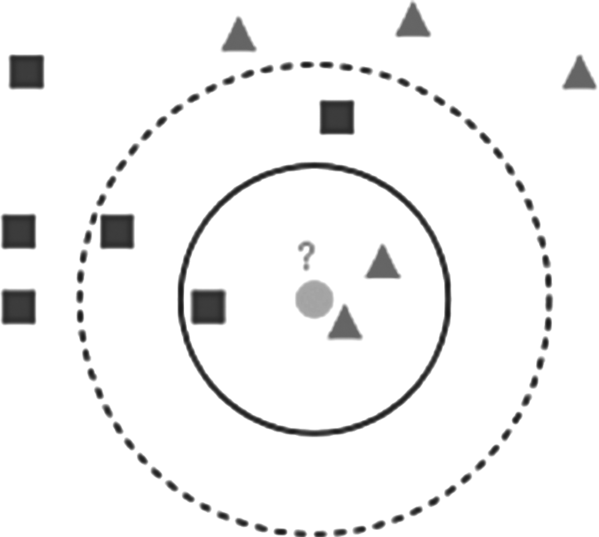
An example of KNN classification with K neighbors K = 3 (solid line circle) and K = 5 (dashed line circle), distance measure is ED. Each triangle represents a training example with two features (x, y), which belongs to class 1. Each square represents a training example with two features (x, y), which belongs to class 2. The gray circle represents a test example with two features (x, y), which belongs to an unknown (?) class, and the KNN needs to predict its class based on the ED distance. ED, Euclidean distance; KNN, K-nearest neighbor.

KNN is simple, but proved to be a highly efficient and effective algorithm for solving various real-life classification problems. However, KNN has got some disadvantages that include the following:

How to find the optimum K value in KNN Algorithm?

High computational time cost as we need to compute the distance between each test sample and all training samples, for each test example we need O(nm) time complexity (number of operations), where n is the number of examples in the training data and m is the number of features for each example.

High memory requirement as we need to store all training samples O(nm) space complexity.

Finally, we need to determine the distance function that is the core of this study.

The first problem was solved either by using all the examples and taking the inverted indexes,²⁹ or using ensemble learning.³⁰ For the second and third problems, many studies have proposed different solutions depending on reducing the size of the training data set, those include and not limited to Refs.,^31–35 or using approximate KNN classification such as those in Arya and Mount³⁶ and Zheng et al.³⁷ Although some previous studies exist in the literature that investigated the fourth problem (see Related Work section), in this study we attempt to investigate the fourth problem on a much larger scale, that is, investigating a large number of distance metrics tested on a large set of problems. In addition, we investigate the effect of noise on choosing the most suitable distance metric to be used by the KNN classifier.

The basic KNN classifier steps can be described as follows:

Algorithm 1: Basic KNN algorithm

Input: Training samples D, test sample d, K

Output: Class label of test sample

1: Compute the distance between d and every sample in D

2: Choose the K samples in D that are nearest to d; denote the set by P (∈D)

3: Assign d the class that is the most frequent class (or the majority class)

Training phase: The training samples and the class labels of these samples are stored, no missing data allowed, no non-numeric data allowed.

Classification phase: Each test sample is classified using majority vote of its neighbors by the following steps: (a)

Distances from the test sample to all stored training samples are calculated using a specific distance function or similarity measure.

(b)

The KNNs of the test sample are selected, where K is a predefined small integer.

(c)

The most repeated class of these KNNs is assigned to the test sample. In other words, a test sample is assigned to the class c if it is the most frequent class label among the K nearest training samples. If K = 1, then the class of the nearest neighbor is assigned to the test sample. KNN algorithm is described by Algorithm 1.

We provide a toy example to illustrate how to compute the KNN classifier. Assuming that we have three training examples, having three attributes for each, and one test example as given in Table 2.

Table 2.

Training and testing data examples

	X1	X2	X3	Class
Training sample (1)	5	4	3	1
Training sample (2)	1	2	2	2
Training sample (3)	1	2	3	2
Test sample	4	4	2	?

Step1: Determine the parameter K = number of the nearest neighbors to be considered. For this example we assume K = 1.

Step 2: Calculate the distance between test sample and all training samples using a specific similarity measure, in this example, ED is used, see Table 3.

Step 3: Sort all examples based on their similarity or distance to the tested example, and then keep only the K similar (nearest) examples as given in Table 4:

Step 4: Based on the minimum distance, the class of the test sample is assigned to be 1. However, if K = 3 for instance, the class will be 2.

Noisy data

The existence of noise in data is mainly related to the way that has been applied to acquire and preprocess data from its environment.³⁸ Noisy data are a corrupted form of data in some way, which leads to partial alteration of the data values. Two main sources of noise can be identified: first, the implicit errors caused by measurement tools, such as using different types of sensors. Second, the random errors caused by batch processes or experts while collecting data, for example, errors during the process document digitization. Based on these two sources of errors, two types of noise can be classified in a given data set³⁹:

Table 3.

Training and testing data examples with distances

	X1	X2	X3	Class	Distance
Training sample (1)	5	4	3	1	$D = \sqrt{{(4 - 5)}^{2} + {(4 - 4)}^{2} + {(2 - 3)}^{2}} = 1.4$
Training sample (2)	1	2	2	2	$D = \sqrt{{(4 - 1)}^{2} + {(4 - 2)}^{2} + {(2 - 2)}^{2}} = 3.6$
Training sample (3)	1	2	3	2	$D = \sqrt{{(4 - 1)}^{2} + {(4 - 2)}^{2} + {(2 - 3)}^{2}} = 3.7$
Test sample	4	4	2	?

Table 4.

Training and testing data examples with distances

	X1	X2	X3	Class	Distance	Rank minimum distance
Training sample (1)	5	4	3	1	1.4	1
Training sample (2)	1	2	2	2	3.6	2
Training sample (3)	1	2	3	2	3.7	3
Test sample	4	4	2	?

Class noise occurs when the sample is incorrectly labeled due to several causes such as data entry errors during labeling process, or the inadequacy of information that is being used to label each sample.

Attribute noise refers to the corruptions in values of 1 or more attributes due to several causes, such as failures in sensor devices, irregularities in sampling, or transcription errors.⁴⁰

The generation of noise can be classified by three main characteristics⁴¹:

The place where the noise is introduced: Noise may affect the attributes, class, training data, and test data separately or in combination.

The noise distribution: The way in which the noise is introduced, for example, uniform or Gaussian.

The magnitude of generated noise values: The extent to which the noise affects the data can be relative to each data value of each attribute, or relative to the standard deviation, minimum, maximum for each attribute.

In this study, we add different noise levels to the tested data sets to find the optimal distance metric that is least affected by this added noise with respect to the KNN classifier performance.

Distance measures review

The first appearance of the word distance can be found in the writings of Aristoteles (384 AC–322 AC), who argued that the word distance means, “It is between extremities that distance is greatest” or “things which have something between them, that is, a certain distance.” In addition, “distance has the sense of dimension [as in space has three dimensions, length, breadth and depth].” Euclid, one of the most important mathematicians of the ancient history, used the word distance only in his third postulate of the Principia⁴²: “Every circle can be described by a centre and a distance.” The distance is a numerical description of how far apart entities are. In data mining, the distance means a concrete way of describing what it means for elements of some space to be close to or far away from each other. Synonyms for distance include farness, dissimilarity, and diversity, and synonyms for similarity include proximity⁴³ and nearness.²²

The distance function between two vectors x and y is a function d(x, y) that defines the distance between both vectors as a non-negative real number. This function is considered as a metric if it satisfies a certain number of properties⁴⁴ that include the following:

Non-negativity: The distance between x and y is always a value ≥0. $d (x, y) \geq 0 .$

Identity of indiscernibles: The distance between x and y is equal to 0 if and only if x is equal to y. $d (x, y) = 0 i f f x = y .$

Symmetry: The distance between x and y is equal to the distance between y and x. $d (x, y) = d (y, x) .$

Triangle inequality: Considering the presence of a third point z, the distance between x and y is always less than or equal to the sum of the distance between x and z and the distance between y and z. $d (x, y) \leq d (x, z) + d (z, y) .$

When the distance is in the range [0,1], the calculation of a corresponding similarity measure s(x, y) is as follows: $s (x, y) = 1 - d (x, y) .$

We consider the 8 major distance families that consist of 54 total distance measures. We categorized these distance measures following a similar categorization done by Cha.⁴³ In what follows, we give the mathematical definitions of distances to measure the closeness between two vectors x and y, where x = (x₁, x₂, …, x_n) and y = (y₁, y₂, …, y_n) having numeric attributes. As an example, we show the computed distance value between the example vectors v1 = {5.1,3.5,1.4,0.3}, v2 = {5.4,3.4,1.7,0.2} as a result in each of these categories of distances reviewed here. Theoretical analysis of these various distance metrics is beyond the scope of this study.

L_p Minkowski distance measures: This family of distances includes three distance metrics that are special cases of Minkowski distance, corresponding to different values of p for this power distance. The Minkowski distance, which is also known as L_p norm, is a generalized metric. It is defined as $D_{M i n k} (x, y) = \sqrt[p]{\sum_{i = 1}^{n} | x_{i} - y_{i} |^{p}},$

where p is a positive value. When p = 2, the distance becomes the ED. When p = 1, it becomes MD. Chebyshev distance (CD) is a variant of Minkowski distance, where p = ∞. x_i is the ith value in vector x and y_i is the ith value in vector y.

1.1.

MD: The MD, also known as L₁ norm, Taxicab norm, rectilinear distance, or City block distance, which was considered by Hermann Minkowski in 19th-century Germany. This distance represents the sum of the absolute differences between the opposite values in vectors. $M D (x, y) = \sum_{i = 1}^{n} | x_{i} - y_{i} | .$

1.2.

CD: CD is also known as maximum value distance,⁴⁵ Lagrange,²² and chessboard distance.⁴⁶ This distance is appropriate in cases when two objects are to be defined as different if they are different in any one dimension.⁴⁷ It is a metric defined on a vector space where distance between two vectors is the greatest of their difference along any coordinate dimension. $C D (x, y) = {max}_{i} | x_{i} - y_{i} | .$

1.3.

ED: Also known as L₂ norm or Ruler distance, which is an extension to the Pythagorean theorem. This distance represents the root of the sum of the square of differences between the opposite values in vectors. $E D (x, y) = \sqrt{\sum_{i = 1}^{n} | x_{i} - y_{i} |^{2}} .$

L_p Minkowski distance measures

Abbreviation	Name	Definition	Result
MD	Manhattan	$\sum_{i = 1}^{n} \| x_{i} - y_{i} \|$	0.8
CD	Chebyshev	max_i\|x_i – y_i\|	0.3
ED	Euclidean	$\sqrt{\sum_{i = 1}^{n} \| x_{i} - y_{i} \|^{2}}$	0.4472

L₁ Distance measures: This distance family depends on mainly finding the absolute difference, the family includes Lorentzian distance (LD), CanD, Sorensen distance (SD), SoD, Kulczynski distance (KD), Mean Character distance (MCD), and Non Intersection distance (NID).

2.1.

LD: LD is represented by the natural log of the absolute difference between two vectors. This distance is sensitive to small changes since the log scale expands the lower range and compresses the higher range. $L D (x, y) = \sum_{i = 1}^{n} l n (1 + | x_{i} - y_{i} |),$

where ln is the natural logarithm, and to ensure that the non-negativity property and to avoid log of 0, 1 is added.

2.2.

CanD: CanD is introduced by⁴⁸ and modified by Lance and Williams.⁴⁹ It is a weighted version of MD, wherein the absolute difference between the attribute values of the vectors x and y is divided by the sum of the absolute attribute values before summing.⁵⁰ This distance is mainly used for positive values. It is very sensitive to small changes near 0, where it is more sensitive to proportional than to absolute differences. Therefore, this characteristic becomes more apparent in higher dimensional space, respectively, with an increasing number of variables. The CanD is often used for data scattered around an origin. $C a n D (x, y) = \sum_{i = 1}^{n} \frac{| x_{i} - y_{i} |}{| x_{i} | + | y_{i} |} .$

2.3.

SD: The SD,⁵¹ also known as Bray–Curtis, is one of the most commonly applied measurements to express relationships in ecology, environmental sciences, and related fields. It is a modified Manhattan metric, wherein the summed differences between the attribute values of the vectors x and y are standardized by their summed attribute values.⁵² When all the vector values are positive, this measure take value between 0 and 1. $S D (x, y) = \frac{\sum_{i = 1}^{n} | x_{i} - y_{i} |}{\sum_{i = 1}^{n} (x_{i} + y_{i})} .$

2.4.

SoD: SoD is one of the distance measures that is widely used to calculate the evolutionary distance.⁵³ It is also known as Ruzicka distance. For binary variables only, this distance is identical to the complement of the Tanimoto (or Jaccard) similarity coefficient.⁵⁴ This distance obeys all four metric properties provided by all attributes that have non-negative values.⁵⁵ $S o D (x, y) = \frac{\sum_{i = 1}^{n} | x_{i} - y_{i} |}{\sum_{i = 1}^{n} max (x_{i}, y_{i})} .$

2.5.

KD: Similar to the SoD, but instead of using the maximum, it uses the minimum function. $K D (x, y) = \frac{\sum_{i = 1}^{n} | x_{i} - y_{i} |}{\sum_{i = 1}^{n} min (x_{i}, y_{i})} .$

2.6.

MCD: Also known as average Manhattan, or Gower distance. $M C D (x, y) = \frac{\sum_{i = 1}^{n} | x_{i} - y_{i} |}{n} .$

2.7.

NID: NID is the complement to the intersection similarity and is obtained by subtracting the intersection similarity from 1. $N I D (x, y) = \frac{1}{2} \sum_{i = 1}^{n} | x_{i} - y_{i} | .$

L₁ Distance measures

Abbreviation	Name	Definition	Result
LD	Lorentzian	$\sum_{i = 1}^{n} l n (1 + \| x_{i} - y_{i} \|)$	0.7153
CanD	Canberra	$\sum_{i = 1}^{n} \frac{\| x_{i} - y_{i} \|}{\| x_{i} \| + \| y_{i} \|}$	0.0381
SD	Sorensen	$\frac{\sum_{i = 1}^{n} \| x_{i} - y_{i} \|}{\sum_{i = 1}^{n} (x_{i} + y_{i})}$	0.0381
SoD	Soergel	$\frac{\sum_{i = 1}^{n} \| x_{i} - y_{i} \|}{\sum_{i = 1}^{n} max (x_{i}, y_{i})}$	0.0734
KD	Kulczynski	$\frac{\sum_{i = 1}^{n} \| x_{i} - y_{i} \|}{\sum_{i = 1}^{n} min (x_{i}, y_{i})}$	0.0792
MCD	Mean Character	$\frac{\sum_{i = 1}^{n} \| x_{i} - y_{i} \|}{n}$	0.2
NID	Non Intersection	$\frac{1}{2} \sum_{i = 1}^{n} \| x_{i} - y_{i} \|$	0.4

Inner product distance measures: Distance measures belonging to this family are calculated by some products of pairwise values from both vectors, this type of distances includes JacD, CosD, Dice distance (DicD), and Chord distance (ChoD).

3.1.

JacD: The JacD measures dissimilarity between sample sets, it is a complementary to the Jaccard similarity coefficient⁵⁶ and is obtained by subtracting the Jaccard coefficient from 1. This distance is a metric.⁵⁷ $J a c D (x, y) = \frac{\sum_{i = 1}^{n} {(x_{i} - y_{i})}^{2}}{\sum_{i = 1}^{n} x_{i}^{2} + \sum_{i = 1}^{n} y_{i}^{2} - \sum_{i = 1}^{n} x_{i} y_{i}} .$

3.2.

CosD: The CosD, also called angular distance, is derived from the cosine similarity that measures the angle between two vectors, where CosD is obtained by subtracting the cosine similarity from 1. $C o s D (x, y) = 1 - \frac{\sum_{i = 1}^{n} x_{i} y_{i}}{\sqrt{\sum_{i = 1}^{n} x_{i}^{2}} \sqrt{\sum_{i = 1}^{n} y_{i}^{2}}} .$

3.3.

DicD: The DicD is derived from the dice similarity,⁵⁸ which is a complementary to the dice similarity and is obtained by subtracting the dice similarity from 1. It can be sensitive to values near 0. This distance is a not a metric, in particular, the property of triangle inequality does not hold. This distance is widely used in information retrieval in documents and biological taxonomy. $D i c D (x, y) = 1 - \frac{2 \sum_{i = 1}^{n} x_{i} y_{i}}{\sum_{i = 1}^{n} x_{i}^{2} + \sum_{i = 1}^{n} y_{i}^{2}} .$

3.4.

ChoD: It is a modification of ED,⁵⁹ which was introduced by Orloci⁶⁰ and to be used in analyzing community composition data.⁶¹ It was defined as the length of the chord joining two normalized points within a hypersphere of radius 1. This distance is one of the distance measures that is commonly used for clustering continuous data.⁶² $C h o D (x, y) = \sqrt{2 - 2 \frac{\sum_{i = 1}^{n} x_{i} y_{i}}{\sum_{i = 1}^{n} x_{i}^{2} \sum_{i = 1}^{n} y_{i}^{2}}} .$

Inner product distance measures family

Abbreviation	Name	Definition	Result
JacD	Jaccard	$\frac{\sum_{i = 1}^{n} {(x_{i} - y_{i})}^{2}}{\sum_{i = 1}^{n} x_{i}^{2} + \sum_{i = 1}^{n} y_{i}^{2} - \sum_{i = 1}^{n} x_{i} y_{i}}$	0.0048
CosD	Cosine	$1 - \frac{\sum_{i = 1}^{n} x_{i} y_{i}}{\sqrt{\sum_{i = 1}^{n} x_{i}^{2}} \sqrt{\sum_{i = 1}^{n} y_{i}^{2}}}$	0.0016
DicD	Dice	$1 - \frac{2 \sum_{i = 1}^{n} x_{i} y_{i}}{\sum_{i = 1}^{n} x_{i}^{2} + \sum_{i = 1}^{n} y_{i}^{2}}$	0.9524
ChoD	Chord	$\sqrt{2 - 2 \frac{\sum_{i = 1}^{n} x_{i} y_{i}}{\sum_{i = 1}^{n} x_{i}^{2} \sum_{i = 1}^{n} y_{i}^{2}}}$	0.0564

Squared chord distance (SCD) measures: Distances that belong to this family are obtained by calculating the sum of geometrics. The geometric mean of two values is the square root of their product. The distances in this family cannot be used with features vector of negative values, this family includes Bhattachayya distance, SCD, Matusita distance (MatD), and Hellinger distance (HeD).

4.1.

BD: The BD measures the similarity of two probability distributions.⁶³ $B D (x, y) = - l n \sum_{i = 1}^{n} \sqrt{x_{i} y_{i}} .$

4.2.

SCD: SCD is mostly used with paleontologists and in studies on pollen. In this distance, the sum of square of square root difference at each point is taken along both vectors, which increases the difference for more dissimilar feature. $S C D (x, y) = \sum_{i = 1}^{n} {(\sqrt{x_{i}} - \sqrt{y_{i}})}^{2} .$

4.3.

MatD: MatD is the square root of the SCD. $M a t D (x, y) = \sqrt{\sum_{i = 1}^{n} {(\sqrt{x_{i}} - \sqrt{y_{i}})}^{2}} .$

4.4.

HeD: HeD also called Jeffries–Matusita distance⁶⁴ was introduced in 1909 by Hellinger,⁶⁵ it is a metric used to measure the similarity between two probability distributions. This distance is closely related to BD. $H e D (x, y) = \sqrt{2 \sum_{i = 1}^{n} {(\sqrt{x_{i}} - \sqrt{y_{i}})}^{2}} .$

SCD measures family

Abbreviation	Name	Definition	Result
BD	Bhattacharyya	$- l n \sum_{i = 1}^{n} \sqrt{x_{i} y_{i}}$	−2.34996
SCD	Squared chord	$\sum_{i = 1}^{n} {(\sqrt{x_{i}} - \sqrt{y_{i}})}^{2}$	0.0297
MatD	Matusita	$\sqrt{\sum_{i = 1}^{n} {(\sqrt{x_{i}} - \sqrt{y_{i}})}^{2}}$	0.1722
HeD	Hellinger	$\sqrt{2 \sum_{i = 1}^{n} {(\sqrt{x_{i}} - \sqrt{y_{i}})}^{2}}$	0.2436

Squared L₂ distance measures: In L₂ distance measure family, the square of difference at each point along both vectors is considered for the total distance, this family includes Squared Euclidean distance (SED), ClaD, Neyman χ² distance (NCSD), Pearson χ² distance (PCSD), Squared χ² distance (SquD), Probabilistic Symmetric χ² distance (PSCSD), Divergence distance (DivD), Additive Symmetric χ² distance (ASCSD), Average distance (AD), Mean Censored Euclidean distance (MCED), and Squared Chi-Squared distance (SCSD).

5.1.

SED: SED is the sum of the squared differences without taking the square root. $S E D (x, y) = \sum_{i = 1}^{n} {(x_{i} - y_{i})}^{2} .$

5.2.

ClaD: The ClaD also called coefficient of divergence was introduced by Clark.⁶⁶ It is the squared root of half of the DivD. $C l a D (x, y) = \sqrt{\sum_{i = 1}^{n} {(\frac{x_{i} - y_{i}}{| x_{i} | + | y_{i} |})}^{2}} .$

5.3.

NCSD: The NCSD⁶⁷ is called a quasi-distance. $N C S D (x, y) = \sum_{i = 1}^{n} \frac{{(x_{i} - y_{i})}^{2}}{x_{i}} .$

5.4.

PCSD: PCSD,⁶⁸ also called χ² distance. $P C S D (x, y) = \sum_{i = 1}^{n} \frac{{(x_{i} - y_{i})}^{2}}{y_{i}} .$

5.5.

SquD: SquD also called triangular discrimination distance. This distance is a quasi-distance. $S q u D (x, y) = \sum_{i = 1}^{n} \frac{{(x_{i} - y_{i})}^{2}}{x_{i} + y_{i}} .$

5.6.

PSCSD: This distance is equivalent to Sangvi χ² distance. $P S C S D (x, y) = 2 \sum_{i = 1}^{n} \frac{{(x_{i} - y_{i})}^{2}}{x_{i} + y_{i}} .$

5.7.

DivD: $D i v D (x, y) = 2 \sum_{i = 1}^{n} \frac{{(x_{i} - y_{i})}^{2}}{{(x_{i} + y_{i})}^{2}} .$

5.8.

ASCSD: Also known as symmetric χ² divergence. $A S C S D (x, y) = 2 \sum_{i = 1}^{n} \frac{{(x_{i} - y_{i})}^{2} (x_{i} + y_{i})}{x_{i} y_{i}} .$

5.9.

AD: The AD, also known as average Euclidean, is a modified version of the ED,⁶² wherein the ED has the following drawback, “if two data vectors have no attribute values in common, they may have a smaller distance than the other pair of data vectors containing the same attribute values,”⁵⁹ so that, this distance was adopted. $A D (x, y) = \sqrt{\frac{1}{n} \sum_{i = 1}^{n} {(x_{i} - y_{i})}^{2}} .$

5.10.

MCED: In this distance, the sum of squared differences between values is calculated and, to get the mean value, the summed value is divided by the total number of values wherein the pairs values do not equal to 0. After that, the square root of the mean should be computed to get the final distance. $M C E D (x, y) = \sqrt{\frac{\sum_{i = 1}^{n} {(x_{i} - y_{i})}^{2}}{\sum_{i = 1}^{n} 1_{x_{i}^{2} + y_{i}^{2} \neq 0}}} .$

5.11.

SCSD: $S C S D (x, y) = \sum_{i = 1}^{n} \frac{{(x_{i} - y_{i})}^{2}}{| x_{i} + y_{i} |} .$

Squared L₂ distance measures family

Abbreviation	Name	Definition	Result
SED	Squared Euclidean	$\sum_{i = 1}^{n} {(x_{i} - y_{i})}^{2}$	0.2
ClaD	Clark	$\sqrt{\sum_{i = 1}^{n} {(\frac{\| x_{i} - y_{i} \|}{x_{i} + y_{i}})}^{2}}$	0.2245
NCSD	Neyman χ²	$\sum_{i = 1}^{n} \frac{{(x_{i} - y_{i})}^{2}}{x_{i}}$	0.1181
PCSD	Pearson χ²	$\sum_{i = 1}^{n} \frac{{(x_{i} - y_{i})}^{2}}{y_{i}}$	0.1225
SquD	Squared χ²	$\sum_{i = 1}^{n} \frac{{(x_{i} - y_{i})}^{2}}{x_{i} + y_{i}}$	0.0591
PSCSD	Probabilistic Symmetric χ²	$2 \sum_{i = 1}^{n} \frac{{(x_{i} - y_{i})}^{2}}{x_{i} + y_{i}}$	0.1182
DivD	Divergence	$2 \sum_{i = 1}^{n} \frac{{(x_{i} - y_{i})}^{2}}{{(x_{i} + y_{i})}^{2}}$	0.1008
ASCSD	Additive Symmetric χ²	$2 \sum_{i = 1}^{n} \frac{{(x_{i} - y_{i})}^{2} (x_{i} + y_{i})}{x_{i} y_{i}}$	0.8054
AD	Average	$\sqrt{\frac{1}{n} \sum_{i = 1}^{n} {(x_{i} - y_{i})}^{2}}$	0.2236
MCED	Mean Censored Euclidean	$\sqrt{\frac{\sum_{i = 1}^{n} {(x_{i} - y_{i})}^{2}}{\sum_{i = 1}^{n} 1_{x_{i}^{2} + y_{i}^{2} \neq 0}}}$	0.2236
SCSD	Squared Chi-Squared	$\sum_{i = 1}^{n} \frac{{(x_{i} - y_{i})}^{2}}{\| x_{i} + y_{i} \|}$	0.0591

Shannon entropy distance measures: The distance measures belonging to this family are related to the Shannon entropy.⁶⁹ These distances include Kullback–Leibler distance (KLD), Jeffreys distance (JefD), KDD, Topsoe distance (TopD), Jensen–Shannon distance (JSD), and Jensen difference distance (JDD).

6.1.

KLD: KLD was introduced by Kullback and Leibler,⁷⁰ it is also known as Kullback–Leibler divergence, relative entropy, or information deviation, which measures the difference between two probability distributions. This distance is not a metric measure, because it is not symmetric. Furthermore, it does not satisfy triangular inequality property, therefore, it is called quasi-distance. Kullback–Leibler divergence has been used in several natural language applications such as for query expansion, language models, and categorization.⁷¹ $K L D (x, y) = \sum_{i = 1}^{n} x_{i} l n \frac{x_{i}}{y_{i}},$

where ln is the natural logarithm.

6.2.

JefD: JefD,⁷² also called J-divergence or KL2-distance, is a symmetric version of the KLD. $J e f D (x, y) = \sum_{i = 1}^{n} (x_{i} - y_{i}) l n \frac{x_{i}}{y_{i}} .$

6.3.

KDD: $K D D (x, y) = \sum_{i = 1}^{n} x_{i} l n \frac{2 x_{i}}{x_{i} + y_{i}} .$

6.4.

TopD: The TopD,⁷³ also called information statistics, is a symmetric version of the KLD. The TopD is twice the Jensen–Shannon divergence. This distance is not a metric, but its square root is a metric. $T o p D (x, y) = \sum_{i = 1}^{n} x_{i} l n (\frac{2 x_{i}}{x_{i} + y_{i}}) + \sum_{i = 1}^{n} y_{i} l n (\frac{2 y_{i}}{x_{i} + y_{i}}) .$

6.5.

JSD: JSD is the square root of the Jensen–Shannon divergence. It is half of the TopD, which uses the average method to make the K divergence symmetric. $J S D (x, y) = \frac{1}{2} [\sum_{i = 1}^{n} x_{i} l n (\frac{2 x_{i}}{x_{i} + y_{i}}) + \sum_{i = 1}^{n} y_{i} l n (\frac{2 y_{i}}{x_{i} + y_{i}})] .$

6.6.

JDD: JDD was introduced by Sibson.⁷⁴ $J D D (x, y) = \frac{1}{2} [\sum_{i = 1}^{n} \frac{x_{i} l n x_{i} + y_{i} l n y_{i}}{2} - (\frac{x_{i} + y_{i}}{2}) l n (\frac{x_{i} + y_{i}}{2})] .$

Shannon entropy distance measures family

Abbreviation	Name	Definition	Result
KLD	Kullback–Leibler	$\sum_{i = 1}^{n} x_{i} l n \frac{x_{i}}{y_{i}}$	−0.3402
JefD	Jeffreys	$\sum_{i = 1}^{n} (x_{i} - y_{i}) l n \frac{x_{i}}{y_{i}}$	0.1184
KDD	K divergence	$\sum_{i = 1}^{n} x_{i} l n \frac{2 x_{i}}{x_{i} + y_{i}}$	−0.1853
TopD	Topsoe	$\sum_{i = 1}^{n} x_{i} l n (\frac{2 x_{i}}{x_{i} + y_{i}}) + \sum_{i = 1}^{n} y_{i} l n (\frac{2 y_{i}}{x_{i} + y_{i}})$	0.0323
JSD	Jensen–Shannon	$\frac{1}{2} [\sum_{i = 1}^{n} x_{i} l n \frac{2 x_{i}}{x_{i} + y_{i}} + \sum_{i = 1}^{n} y_{i} l n \frac{2 y_{i}}{x_{i} + y_{i}}]$	0.014809
JDD	Jensen difference	$\frac{1}{2} [\sum_{i = 1}^{n} \frac{x_{i} l n x_{i} + y_{i} l n y_{i}}{2} - (\frac{x_{i} + y_{i}}{2}) l n (\frac{x_{i} + y_{i}}{2})]$	0.0074

Vicissitude distance measures: Vicissitude distance family consists of four distances, Vicis-Wave Hedges distance (VWHD), Vicis Symmetric distance (VSD), Max Symmetric χ² distance (MSCSD), and Min Symmetric χ² distance (MiSCSD). These distances were generated from syntactic relationship for the aforementioned distance measures.

7.1.

VWHD: The so-called Wave-Hedges distance has been applied to compressed image retrieval,⁷⁵ content-based video retrieval,⁷⁶ time series classification,⁷⁷ image fidelity,⁷⁸ finger print recognition,⁷⁹ etc. Interestingly, the source of the “Wave-Hedges” metric has not been correctly cited, and some of the previously mentioned resources allude to it incorrectly as given by Hedges.⁸⁰ The source of this metric eludes the authors, despite best efforts otherwise. Even the name of the distance “Wave-Hedges” is questioned.²⁶ $V W H D (x, y) = \sum_{i = 1}^{n} \frac{| x_{i} - y_{i} |}{min (x_{i}, y_{i})} .$

7.2.

VSD: VSD is defined by three formulas, VSDF1, VSDF2, and VSDF3 as the following: $\begin{matrix} V S D F 1 (x, y) = \sum_{i = 1}^{n} \frac{{(x_{i} - y_{i})}^{2}}{min {(x_{i}, y_{i})}^{2}}, \\ V S D F 2 (x, y) = \sum_{i = 1}^{n} \frac{{(x_{i} - y_{i})}^{2}}{min (x_{i}, y_{i})}, \\ V S D F 3 (x, y) = \sum_{i = 1}^{n} \frac{{(x_{i} - y_{i})}^{2}}{max (x_{i}, y_{i})} \end{matrix} .$

7.3.

MSCSD: $M S C D (x, y) = max (\sum_{i = 1}^{n} \frac{{(x_{i} - y_{i})}^{2}}{x_{i}}, \sum_{i = 1}^{n} \frac{{(x_{i} - y_{i})}^{2}}{y_{i}}) .$

7.4.

MiSCSD: $M i S C S D (x, y) = min (\sum_{i = 1}^{n} \frac{{(x_{i} - y_{i})}^{2}}{x_{i}}, \sum_{i = 1}^{n} \frac{{(x_{i} - y_{i})}^{2}}{y_{i}}) .$

Vicissitude distance measures family

Abbreviation	Name	Definition	Result
VWHD	Vicis-Wave Hedges	$\sum_{i = 1}^{n} \frac{\| x_{i} - y_{i} \|}{min (x_{i}, y_{i})}$	0.8025
VSDF1	Vicis Symmetric1	$\sum_{i = 1}^{n} \frac{{(x_{i} - y_{i})}^{2}}{min {(x_{i}, y_{i})}^{2}}$	0.3002
VSDF2	Vicis Symmetric2	$\sum_{i = 1}^{n} \frac{{(x_{i} - y_{i})}^{2}}{min (x_{i}, y_{i})}$	0.1349
VSDF3	Vicis Symmetric3	$\sum_{i = 1}^{n} \frac{{(x_{i} - y_{i})}^{2}}{max (x_{i}, y_{i})}$	0.1058
MSCSD	Max Symmetric χ²	$max (\sum_{i = 1}^{n} \frac{{(x_{i} - y_{i})}^{2}}{x_{i}}, \sum_{i = 1}^{n} \frac{{(x_{i} - y_{i})}^{2}}{y_{i}})$	0.1225
MiSCSD	Min Symmetric χ²	$min (\sum_{i = 1}^{n} \frac{{(x_{i} - y_{i})}^{2}}{x_{i}}, \sum_{i = 1}^{n} \frac{{(x_{i} - y_{i})}^{2}}{y_{i}})$	0.1181

Other distance measures: These metrics exhibit distance measures utilizing multiple ideas or measures from previous distance measures, these include and not limited to Average distance (L₁, L_∞) (AvgD), Kumar–Johnson distance (KJD), Taneja distance (TanD), Pearson distance (PeaD), CorD, Squared Pearson distance (SPeaD), HamD, Hausdorff distance (HauD), χ² statistic distance (CSSD), Whittaker's index of association distance (WIAD), Meehl distance (MeeD), Motyka distance (MotD), and HasD.

8.1.

AvgD: AvgD is the average of MD and CD. $A v g D (x, y) = \frac{\sum_{i = 1}^{n} | x_{i} - y_{i} | + {max}_{i} | x_{i} - y_{i} |}{2} .$

8.2.

KJD: $K J D (x, y) = \sum_{i = 1}^{n} (\frac{{(x_{i}^{2} + y_{i}^{2})}^{2}}{2 {(x_{i} y_{i})}^{3 ∕ 2}}) .$

8.3.

TanD⁸¹: $T J D (x, y) = \sum_{i = 1}^{n} (\frac{x_{i} + y_{i}}{2}) l n (\frac{x_{i} + y_{i}}{2 \sqrt{x_{i} y_{i}}}) .$

8.4.

PeaD: The PeaD is derived from the Pearson's correlation coefficient, which measures the linear relationship between two vectors.⁸² This distance is obtained by subtracting the Pearson's correlation coefficient from 1. $P e a D (x, y) = 1 - \frac{\sum_{i = 1}^{n} (x_{i} - \bar{x}) (y_{i} - ȳ)}{\sqrt{\sum_{i = 1}^{n} {(x_{i} - \bar{x})}^{2} ⋆ \sum_{i = 1}^{n} {(y_{i} - ȳ)}^{2}}},$

where $\bar{x} = \frac{1}{n} \sum_{i = 1}^{n} x_{i}$ .

8.5.

CorD: CorD is a version of the PeaD, where the PeaD is scaled to obtain a distance measure in the range between 0 and 1. $C o r D (x, y) = \frac{1}{2} (1 - \frac{\sum_{i = 1}^{n} (x_{i} - \bar{x}) (y_{i} - ȳ)}{\sqrt{\sum_{i = 1}^{n} {(x_{i} - \bar{x})}^{2}} \sqrt{\sum_{i = 1}^{n} {(y_{i} - ȳ)}^{2}}}) .$

8.6.

SPeaD: $S P e a D (x, y) = 1 - {(\frac{\sum_{i = 1}^{n} (x_{i} - \bar{x}) (y_{i} - ȳ)}{\sqrt{\sum_{i = 1}^{n} {(x_{i} - \bar{x})}^{2}} \sqrt{\sum_{i = 1}^{n} {(y_{i} - ȳ)}^{2}}})}^{2} .$

8.7.

HamD: HamD⁸³ is a distance metric that measures the number of mismatches between two vectors. It is mostly used for nominal data, string, and bit-wise analyses, and also can be useful for numerical data. $H a m D (x, y) = \sum_{i = 1}^{n} 1_{x_{i} \neq y_{i}} .$

8.8.

HauD: $H a u D (x, y) = max (h (x, y), h (y, x)),$

where h(x, y) = max_xi∈x min_yi∈y||x_i – y_i||, and ||⋅|| is the vector norm (e.g., L₂ norm). The function h(x, y) is called the directed HauD from x to y. The HauD(x, y) measures the degree of mismatch between the sets x and y by measuring the remoteness between each point x_i and y_i and vice versa.

8.9.

CSSD: The CSSD was used for image retrieval,⁸⁴ histogram,⁸⁵ etc. $C S S D (x, y) = \sum_{i = 1}^{n} \frac{x_{i} - m_{i}}{m_{i}},$

where $m_{i} = \frac{x_{i} + y_{i}}{2}$ .

8.10.

WIAD: WIAD was designed for species abundance data.⁸⁶ $W I A D (x, y) = \frac{1}{2} \sum_{i = 1}^{n} | \frac{x_{i}}{\sum_{i = 1}^{n} x_{i}} - \frac{y_{i}}{\sum_{i = 1}^{n} y_{i}} | .$

8.11.

MeeD: MeeD depends on one consecutive point in each vector. $M e e D (x, y) = \sum_{i = 1}^{n - 1} {(x_{i} - y_{i} - x_{i + 1} + y_{i + 1})}^{2} .$

8.12.

MotD: $M o t D (x, y) = \frac{\sum_{i = 1}^{n} max (x_{i}, y_{i})}{\sum_{i = 1}^{n} (x_{i} + y_{i})} .$

8.13.

HasD: This is a nonconvex distance introduced by Hassanat²⁶ $H a s D (x, y) = \sum_{i = 1}^{n} D (x_{i}, y_{i}),$

where $D (x, y) = \{\begin{matrix} 1 - \frac{1 + min (x_{i}, y_{i})}{1 + max (x_{i}, y_{i})}, & min (x_{i}, y_{i}) \geq 0 \\ 1 - \frac{1 + min (x_{i}, y_{i}) + | min (x_{i}, y_{i}) |}{1 + max (x_{i}, y_{i}) + | min (x_{i}, y_{i}) |}, & min (x_{i}, y_{i}) < 0 \end{matrix} .$

As can be seen, HasD is bounded by [0,1]. It reaches 1 when the maximum value approaches infinity assuming the minimum is finite, or when the minimum value approaches minus infinity assuming the maximum is finite. This is shown in Figure 2 and the following equations. ${lim}_{max (A_{i}, B_{i}) \to \infty} D (A_{i}, B_{i}) = {lim}_{max (A_{i}, B_{i}) \to - \infty} D (A_{i}, B_{i}) = 1 .$

By satisfying all the metric properties, this distance was proved to be a metric by Hassanat.²⁶ In this metric no matter what the difference between two values is, the distance will be in the range of 0 to 1. So the maximum distance approaches the dimension of the tested vectors; therefore, the increase in dimensions increases the distance linearly in the worst case.

Other distance measures family

Abbreviation	Name	Definition	Result
AvgD	Average (L₁, L_∞)	$\frac{\sum_{i = 1}^{n} \| x_{i} - y_{i} \| + {max}_{i} \| x_{i} - y_{i} \|}{2}$	0.55
KJD	Kumar–Johnson	$\sum_{i = 1}^{n} (\frac{{(x_{i}^{2} + y_{i}^{2})}^{2}}{2 {(x_{i} y_{i})}^{3 ∕ 2}})$	21.2138
TanD	Taneja	$\sum_{i = 1}^{n} (\frac{x_{i} + y_{i}}{2}) l n (\frac{x_{i} + y_{i}}{2 \sqrt{x_{i} y_{i}}})$	0.0149
PeaD	Pearson	$1 - \frac{\sum_{i = 1}^{n} (x_{i} - \bar{x}) (y_{i} - ȳ)}{\sqrt{\sum_{i = 1}^{n} {(x_{i} - \bar{x})}^{2} ⋆ \sum_{i = 1}^{n} {(y_{i} - ȳ)}^{2}}}$
		$\bar{x} = \frac{1}{n} \sum_{i = 1}^{n} x_{i}$	0.9684
CorD	Correlation	$\frac{1}{2} (1 - \frac{\sum_{i = 1}^{n} (x_{i} - \bar{x}) (y_{i} - ȳ)}{\sqrt{\sum_{i = 1}^{n} {(x_{i} - \bar{x})}^{2}} \sqrt{\sum_{i = 1}^{n} {(y_{i} - ȳ)}^{2}}})$	0.4842
SPeaD	Squared Pearson	$1 - {(\frac{\sum_{i = 1}^{n} (x_{i} - \bar{x}) (y_{i} - ȳ)}{\sqrt{\sum_{i = 1}^{n} {(x_{i} - \bar{x})}^{2}} \sqrt{\sum_{i = 1}^{n} {(y_{i} - ȳ)}^{2}}})}^{2}$	0.999
HamD	Hamming	$\sum_{i = 1}^{n} 1_{x_{i} \neq y_{i}}$	4
HauD	Hausdorff	Max [h(x, y), h(y, x)]
		h(x, y) = max_xi∈x min_yi∈y \|\|x_i – y_i\|\|	0.3
CSSD	χ² statistic	$\sum_{i = 1}^{n} \frac{x_{i} - m_{i}}{m_{i}}, m_{i} = \frac{x_{i} + y_{i}}{2}$	0.0894
WIAD	Whittaker's index of association	$\frac{1}{2} \sum_{i = 1}^{n} \| \frac{x_{i}}{\sum_{i = 1}^{n} x_{i}} - \frac{y_{i}}{\sum_{i = 1}^{n} y_{i}} \|$	1.9377
MeeD	Meehl	$\sum_{i = 1}^{n - 1} {(x_{i} - y_{i} - x_{i + 1} + y_{i + 1})}^{2}$	0.48
MotD	Motyka	$\frac{\sum_{i = 1}^{n} max (x_{i}, y_{i})}{\sum_{i = 1}^{n} (x_{i} + y_{i})}$	0.5190
HasD	Hassanat	$\sum_{i = 1}^{n} D (x_{i}, y_{i})$
		$= \{\begin{matrix} 1 - \frac{1 + min (x_{i}, y_{i})}{1 + max (x_{i}, y_{i})}, & min (x_{i}, y_{i}) \geq 0 \\ 1 - \frac{1 + min (x_{i}, y_{i}) + \| min (x_{i}, y_{i}) \|}{1 + max (x_{i}, y_{i}) + \| min (x_{i}, y_{i}) \|}, & min (x_{i}, y_{i}) < 0 \end{matrix}$	0.2571

Experimental Framework

Data sets used for experiments

The experiments were done on 28 data sets that represent real-life classification problems, obtained from the UCI Machine Learning Repository.⁸⁷ The UCI Machine Learning Repository is a collection of databases, domain theories, and data generators that are used by the machine learning community for the empirical analysis of machine learning algorithms. The database was created in 1987 by David Aha and fellow graduate students at UCI. Since that time, it has been widely used by students, educators, and researchers all over the world as a primary source of machine learning data sets.

FIG. 2.

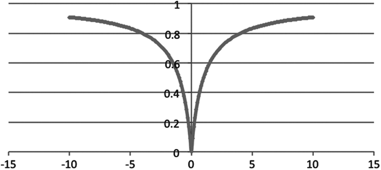
Representation of HasD between the point 0 and n, where n belongs to [−10,10]. HasD, Hassanat distance.

Each data set consists of a set of examples. Each example is defined by a number of attributes and all the examples inside the data are represented by the same number of attributes. One of these attributes is called the class attribute, which contains the class value (label) of the data, whose values are predicted for testing the examples. Short description of all the data sets used is provided in Table 5.

Table 5.

Description of the real-world data sets used (from the UCI machine learning repository)

Name	#E	#F	#C	Data type	Min	Max
Heart	270	25	2	Real and integer	0	564
Balance	625	4	3	Positive integer	1	5
Cancer	683	9	2	Positive integer	0	9
German	1000	24	2	Positive integer	0	184
Liver	345	6	2	Real and integer	0	297
Vehicle	846	18	4	Positive integer	0	1018
Vote	399	10	2	Positive integer	0	2
BCW	699	10	2	Positive integer	1	13,454,352
Haberman	306	3	2	Positive integer	0	83
Letter recognition	20,000	16	26	Positive integer	0	15
Wholesale	440	7	2	Positive integer	1	112,151
Australian	690	42	2	Positive real	0	100,001
Glass	214	9	6	Positive real	0	75.41
Sonar	208	60	2	Positive real	0	1
Wine	178	13	3	Positive real	0.13	1680
EEG	14,980	14	2	Positive real	86.67	715,897
Parkinson	1040	27	2	Positive real	0	1490
Iris	150	4	3	Positive real	0.1	7.9
Diabetes	768	8	2	Real and integer	0	846
Monkey1	556	17	2	Binary	0	1
Ionosphere	351	34	2	Real	−1	1
Phoneme	5404	5	2	Real	−1.82	4.38
Segmen	2310	19	7	Real	−50	1386.33
Vowel	528	10	11	Real	−5.21	5.07
Wave21	5000	21	3	Real	−4.2	9.06
Wave40	5000	40	3	Real	−3.97	8.82
Banknote	1372	4	2	Real	−13.77	17.93
QSAR	1055	41	2	Real	−5.256	147

BCW, Breast Cancer Wisconsin; #C, number of classes; #E, number of examples; #F, number of features; Max, maximum; Min, minimum; QSAR, quantitative structure activity relationships.

Experimental setup

Each data set is divided into two data sets, one for training and the other for testing. For this purpose, 34% of the data set is used for testing and 66% of the data set is dedicated for training. The value of K is set to 1 for simplicity. The 34% of the data, which were used as a test sample, were chosen randomly, and each experiment on each data set was repeated 10 times to obtain random examples for testing and training. The overall experimental framework is shown in Figure 3. Our experiments are divided into two major parts:

FIG. 3.

The framework of our experiments for discerning the effect of various distances on the performance of KNN classifier. 1-NN, 1-nearest neighbor.

The first part of experiments aim to find the best distance measures to be used by KNN classifier without any noise in the data sets. We used all the 54 distances that were reviewed in Distance Measures Review section.

The second part of experiments aim to find the best distance measure to be used by KNN classifier in the case of noisy data. In this study, we define the “best” method as the method that performs with the highest accuracy. We added noise into each data set at various levels of noise. The experiments in the second part were conducted using the top 10 distances, those that achieved the best results in the first part of experiments. Therefore, to create a noisy data set from the original data set, a level of noise x% is selected in the range of (10%–90%), the level of noise means the number of examples that need to be noisy, the amount of noise is selected randomly between the minimum and maximum values of each attribute, all attributes for each examples are corrupted by a random noise, the number of noisy examples is selected randomly. Algorithm 2 describes the process of corrupting data with random noise to be used for further experiments for the purposes of this study.

Algorithm 2: Create noisy data set

Input: Original data set D, level of noise x% [10%–90%]

Output: Noisy data set

1: Number of noisy examples: N = x%^* number of examples in D

2: Array NoisyExample [N]

3: for K = 1 to N do

4: Randomly choose an example number as E from D

5: if E is chosen previously then

6: Go to Step 4

7: else

8: NoisyExample [k] = E

9: for each attribute A_i do do

10: for each NoisyExample NE_j do do

11: RV = Random value between Min(A_i) and Max(A_i)

12: NE_jA_j = RV

Performance evaluation measures

Different measures are available for evaluating the performance of classifiers. In this study, three measures were used: accuracy, precision, and recall. Accuracy is calculated to evaluate the overall classifier performance. It is defined as the ratio of the test samples that are correctly classified to the number of tested examples, $A c c u r a c y = \frac{N u m b e r o f c o r r e c t c l a s s i f i c a t i o n s}{T o t a l n u m b e r o f t e s t s a m p l e s} .$ (1)

To assess the performance with respect to every class in a data set, we compute precision and recall measures. Precision (or positive predictive value) is the fraction of retrieved instances that are relevant, whereas recall (or sensitivity) is the fraction of relevant instances that are retrieved. These measures can be constructed by computing the following:

True positive (TP): The number of correctly classified examples of a specific class (as we calculate these measures for each class).

True negative (TN): The number of correctly classified examples that were not belonging to the specific class.

False positive (FP): The number of examples that are incorrectly assigned to the specific class.

False negative (FN): The number of examples that are incorrectly assigned to another class.

The precision and recall of a multiclass classification system are defined by $A v e r a g e P r e c i s i o n = \frac{1}{N} \sum_{i = 1}^{N} \frac{T P_{i}}{T P_{i} + F P_{i}},$ (2) $A v e r a g e R e c a l l = \frac{1}{N} \sum_{i = 1}^{N} \frac{T P_{i}}{T P_{i} + F N_{i}},$ (3)

where N is the number of classes, TP_i is the number of TP for class i, FN_i is the number of FN for class i, and FP_i is the number of FP for class i.

These performance measures can be derived from the confusion matrix. The confusion matrix is represented by a matrix that shows the predicted and actual classification. The matrix is n × n, where n is the number of classes. The structure of confusion matrix for multiclass classification is given by $(\begin{matrix} P r e d i c t e d C l a s s \\ C l a s s i f i e d a s c_{1} & C l a s s i f i e d a s c_{12} & \dots & C l a s s i f i e d a s c_{1 n} \\ A c t u a l C l a s s c_{1} & c_{11} & c_{12} & \dots & c_{1 n} \\ A c t u a l C l a s s c_{2} & c_{21} & c_{22} & \dots & c_{2 n} \\ ⋮ & ⋮ & ⋮ & ⋮ & ⋮ \\ A c t u a l C l a s s c_{n} & c_{n 1} & c_{n 2} & \dots & c_{n n} \end{matrix})$ (4)

This matrix reports the number of FPs, FNs, TPs, and TNs that are defined through elements of the confusion matrix as follows: $T P_{i} = c_{i i},$ (5) $F P_{i} = \sum_{k = 1}^{N} c_{k i} - T P_{i},$ (6) $F N_{i} = \sum_{k = 1}^{N} c_{i k} - T P_{i},$ (7) $T N_{i} = \sum_{k = 1}^{N} \sum_{f = 1}^{N} c_{k f} - T P_{i} - F P_{i} - F N_{i} .$ (8)

Accuracy, precision, and recall are calculated for the KNN classifier using all the similarity measures and distance metrics discussed in Distance Measures Review section, on all the data sets described in Table 5, this is to compare and assess the performance of the KNN classifier using different distance metrics and similarity measures.

Experimental results and discussion

For the purposes of this review, two sets of experiments were conducted. The aim of the first set is to compare the performance of the KNN classifiers when used with each of the 54 distances and similarity measures reviewed in Distance Measures Review section without any noise. The second set of experiments is designed to find the most robust distance that affected the least with different noise levels.

Without noise

A number of different predefined distance families were used in this set of experiments. The accuracy of each distance on each data set is averaged for 10 runs. The same technique is followed for all other distance families to report accuracy, recall, and precision of the KNN classifier for each distance on each data set. The average values for each of 54 distances considered in the article are summarized in Table 6, where HasD obtained the highest overall average.

Table 6.

Average accuracies, recalls, and precisions over all data sets for each distance

Distance	Accuracy	Recall	Precision	Distance	Accuracy	Recall	Precision
ED	0.8001	0.6749	0.6724	PSCSD	0.6821	0.5528	0.5504
MD	0.8113	0.6831	0.681	DivD	0.812	0.678	0.6768
CD	0.7708	0.656	0.6467	ClaD	0.8227	0.6892	0.6871
LD	0.8316	0.6964	0.6934	ASCSD	0.6259	0.4814	0.4861
CanD	0.8282	0.6932	0.6916	SED	0.8001	0.6749	0.6724
SD	0.7407	0.6141	0.6152	AD	0.8001	0.6749	0.6724
SoD	0.7881	0.6651	0.6587	SCSD	0.8275	0.693	0.6909
KD	0.6657	0.5369	0.5325	MCED	0.7973	0.6735	0.6704
MCD	0.8113	0.6831	0.681	TopD	0.6793	0.461	0.4879
NID	0.8113	0.6831	0.681	JSD	0.6793	0.461	0.4879
CosD	0.803	0.6735	0.6693	JDD	0.7482	0.5543	0.5676
ChoD	0.7984	0.662	0.6647	JefD	0.7951	0.6404	0.6251
JacD	0.8024	0.6756	0.6739	KLD	0.513	0.3456	0.3808
DicD	0.8024	0.6756	0.6739	KDD	0.5375	0.3863	0.4182
SCD	0.8164	0.65	0.4813	KJD	0.6501	0.4984	0.5222
HeD	0.8164	0.65	0.6143	TanD	0.7496	0.5553	0.5718
BD	0.4875	0.3283	0.4855	AvgD	0.8084	0.6811	0.6794
MatD	0.8164	0.65	0.5799	HamD	0.6413	0.5407	0.5348
VWHD	0.6174	0.4772	0.5871	MeeD	0.415	0.1605	0.3333
VSDF1	0.7514	0.6043	0.5125	WIAD	0.812	0.6815	0.6804
VSDF2	0.6226	0.4828	0.5621	HauD	0.5967	0.4793	0.4871
VSDF3	0.7084	0.5791	0.5621	CSSD	0.4397	0.2538	0.332
MSCSD	0.7224	0.5876	0.3769	SPeaD	0.8023	0.6711	0.6685
MiSCSD	0.6475	0.5137	0.5621	CorD	0.803	0.6717	0.6692
PCSD	0.6946	0.5709	0.5696	PeaD	0.759	0.6546	0.6395
NCSD	0.6536	0.5144	0.5148	MotD	0.7407	0.6141	0.6152
SquD	0.6821	0.5528	0.5504	HasD	0.8394	0.7018	0.701

Bold values signify the best performance, which is the highest accuracy, precision or recall.

HasD obtained the highest overall average.

AD, Average distance; ASCSD, Additive Symmetric χ²; AvgD, Average (L₁, L_∞) distance; BD, Bhattacharyya distance; CanD, Canberra distance; CD, Chebyshev distance; ChoD, Chord distance; ClaD, Clark distance; CorD, Correlation distance; CosD, Cosine distance; CSSD, χ² statistic distance; DicD, Dice distance; DivD, Divergence distance; ED, Euclidean distance; HamD, Hamming distance; HasD, Hassanat distance; HauD, Hausdorff distance; HeD, Hellinger distance; JacD, Jaccard distance; JDD, Jensen difference distance; JefD, Jeffreys distance; JSD, Jensen–Shannon distance; KD, Kulczynski distance; KDD, K divergence distance; KJD, Kumar–Johnson distance; KLD, Kullback–Leibler distance; LD, Lorentzian distance; MatD, Matusita distance; MCD, Mean Character distance; MCED, Mean Censored Euclidean distance; MD, Manhattan distance; MeeD, Meehl distance; MiSCSD, Min symmetric χ² distance; MotD, Motyka distance; MSCSD, Max symmetric χ² distance; NCSD, Neyman χ² distance; NID, Non Intersection distance; PCSD, Pearson χ² distance; PeaD, Pearson distance; PSCSD, Probabilistic Symmetric χ² distance; SCD, Squared chord distance; SCSD, Squared Chi-Squared; SD, Sorensen distance; SED, Squared Euclidean distance; SoD, Soergel distance; SPeaD, Squared Pearson distance; SquD, Squared χ² distance; TanD, Taneja distance; TopD, Topsoe distance; VSD, Vicis symmetric distance; VWHD, Vicis-Wave Hedges distance; WIAD, Whittaker's index of association distance.

Table 7 shows the distances that obtained the highest accuracy on each data set. Based on these results we summarize the following observations.

Table 7.

The highest accuracy in each data set

Data set	Distance	Accuracy
Australian	CanD	0.8209
Balance	ChoD, SPeaD, CorD, CosD	0.933
Banknote	CD, DicD, JacD	1
BCW	HasD	0.9624
Cancer	HasD	0.9616
Diabetes	MSCSD	0.6897
Glass	LD, MCED	0.7111
Haberman	KLD	0.7327
Heart	HamD	0.7714
Ionosphere	HasD	0.9025
Liver	VSDF1	0.6581
Monkey1	WIAD	0.9497
Parkinson	VSDF1	0.9997
Phoneme	VSDF1	0.898
QSAR	HasD	0.8257
Segmen	SoD, SD	0.9676
Sonar	MiSCSD	0.8771
Vehicle	LD	0.6913
Vote	ClaD, DivD	0.9178
Vowel	LD	0.9771
Wholesale	AvgD	0.8866
Wine	CanD	0.985
German	ASCSD	0.71
Iris	ChoD, SPeaD, CorD, CosD	0.9588
Wave21	ED, AD, MCED, SED	0.7774
Egg	ChoD, SPeaD, CorD, CosD	0.9725
Wave40	ED, AD, MCED, SED	0.7587
Letter recognition	JacD, DicD	0.9516

The distance measures in L₁ family outperformed the other distance families in five data sets. LD achieved the highest accuracy in two data sets, namely on Vehicle and Vowel with average accuracies of 69.13% and 97.71%, respectively. In contrast, CanD achieved the highest accuracy in two data sets, Australian and Wine data sets achieved average accuracies of 82.09% and 98.5%, respectively. SD and SoD achieved the highest accuracy on Segmen data set with an average accuracy of 96.76%. Among the L_p Minkowski and L₁ distance families, the MD, NID, and MCD achieved similar performance with overall accuracies on all data sets: this is due to the similarity between these distances.

In inner product family, JacD and DicD outperform all other tested distances on Letter recognition data set with an average accuracy of 95.16%. Among the L_p Minkowski and L₁ distance families, the CD, JacD, and DicD outperform the other tested distances on the Banknote data set with an average accuracy of 100%.

In Squared chord family, MatD, SCD, and HeD achieved similar performance with overall accuracies on all data sets, this is expected because these distances are very similar.

In Squared L₂ distance measures family, SquD and PSCSD achieved similar performance with overall accuracy in all data sets: this is due to the similarity between these two distances. The distance measures in this family outperform the other distance families on two data sets, namely, ASCSD achieved the highest accuracy on the German data set with an average accuracy of 71%. ClaD and DivD achieved the highest accuracy on the Vote data set with an average accuracy of 91.87%. Among the L_p Minkowski and Squared L₂ distance measures family, ED, SED, and AD achieved similar performance in all data sets: this is due to the similarity between these three distances. Also, these distances and MCED outperform the other tested distances in two data sets, Wave21 and Wave40, with average accuracies of 77.74% and 75.87%, respectively. Among the L₁ distance and Squared L₂ families, MCED and LD achieved the highest accuracy on the Glass data set with an average accuracy of 71.11%.

In Shannon entropy distance measures family, JSD and TopD achieved similar performance with overall accuracies on all data sets: this is due to similarity between both of the distances, as TopD is twice the JSD. KLD outperforms all the tested distances on Haberman data set with an average accuracy of 73.27%.

The Vicissitude distance measures family outperform the other distance families on five data sets, namely, VSDF1 achieved the highest accuracy in three data sets, Liver, Parkinson, and Phoneme with accuracies of 65.81%, 99.97%, and 89.8%, respectively. MSCSD achieved the highest accuracy on the Diabetes data set with an average accuracy of 68.79%. MiSCSD also achieved the highest accuracy on Sonar data set with an average accuracy of 87.71%.

The other distance measures family outperforms all other distance families in seven data sets. The WIAD achieved the highest accuracy on Monkey1 data set with an average accuracy of 94.97%. The AvgD also achieved the highest accuracy on the Wholesale data set with an average accuracy of 88.66%. HasD also achieved the highest accuracy in four data sets, namely, Cancer, Breast Cancer Wisconsin (BCW), Ionosphere, and quantitative structure activity relationships (QSAR) with average accuracies of 96.16%, 96.24%, 90.25%, and 82.57%, respectively. Finally, HamD achieved the highest accuracy on the Heart data set with an average accuracy of 77.14%. Among the inner product and other distance measures families, SPeaD, CorD, ChoD, and CosD outperform other tested distances in three data sets, namely, Balance, Iris, and Egg with average accuracies of 94.3%, 95.88%, and 97.25%, respectively.

Table 8 shows the distances that obtained the highest recall on each data set. Based on these results, we summarize the following observations.

Table 8.

The highest recall in each data set

Data set	Distance	Recall
Australian	CanD	0.8183
Balance	ChoD, SPeaD, CorD, CosD	0.6437
Banknote	CD, DicD, JacD	1
BCW	HasD	0.3833
Cancer	HasD	0.9608
Diabetes	MSCSD	0.4371
Glass	LD	0.5115
Haberman	DicD, JacD	0.3853
Heart	HamD	0.5122
Ionosphere	LD	0.6152
Liver	VSDF1	0.4365
Monkey1	WIAD	0.9498
Parkinson	VSDF1	0.9997
Phoneme	VSDF1	0.8813
QSAR	HasD	0.8041
Segmen	SoD, SD	0.8467
Sonar	MiSCSD	0.5888
Vehicle	LD	0.5485
Vote	ClaD, DivD	0.9103
Vowel	LD	0.9768
Wholesale	PCSD	0.5816
Wine	CanD	0.7394
German	ASCSD	0.4392
Iris	ChoD, SPeaD, CorD, CosD	0.9592
Wave21	ED, AD, MCED, SED	0.7771
Egg	ChoD, SPeaD, CorD, CosD	0.9772
Wave40	ED, AD, MCED, SED	0.7588
Letter recognition	VSDF2	0.9514

The L₁ distance measures family outperforms the other distance families in seven data sets, for example, CanD achieved the highest recalls in two data sets, Australian and Wine with 81.83% and 73.94% average recalls respectively. LD also achieved the highest recalls on four data sets, Glass, Ionosphere, Vehicle, and Vowel with 51.15%, 61.52%, 54.85%, and 97.68% average recalls, respectively. SD and SoD achieved the highest recall on Segmen data set with 84.67% average recall. Among the L_p Minkowski and L₁ distance families, MD, NID, and MCD achieved similar performance as expected, due to their similarity.

In Inner Product distance measures family, JacD and DicD outperform all other tested distances in Heberman data set with 38.53% average recall. Among the L_p Minkowski and Inner Product distance measures families, CD, JacD, and DicD also outperform the other tested distances in the Banknote data set with 100% average recall.

In SCD measures family, MatD, SCD, and HeD achieved similar performance: this is due to similarity of their equations as clarified previously.

The Squared L₂ distance measures family outperforms the other distance families on two data sets, namely, ClaD and DivD outperform the other tested distances on Vote data set with 91.03% average recall. PCSD outperforms the other tested distances on Wholesale data set with 58.16% average recall. ASCSD also outperforms the other tested distances on German data set with 43.92% average recall. Among the L_p Minkowski and Squared L₂ distance measures families, ED, SED, and AD achieved similar performance in all data sets: this is due to similarity of their equations as clarified previously. These distances and MCED distance outperform the other tested distances in two data sets, namely, Wave21 and Wave40 with 77.71% and 75.88% average recalls, respectively.

In Shannon entropy distance measures family, JSD and TopD achieved similar performance as expected, due to their similarity.

The Vicissitude distance measures family outperforms the other distance families in six data sets. VSDF1 achieved the highest recall on three data sets: Liver, Parkinson, and Phoneme data sets with 43.65%, 99.97%, 88.13% average recalls, respectively. MSCSD achieved the highest recall on Diabetes data set with 43.71% average recall. MiSCSD also achieved the highest recall on Sonar data set with 58.88% average recall. VSDF2 achieved the highest recall on Letter recognition data set with 95.14% average recall.

The other distance measures family outperforms all other distance families in five data sets. Particularly, HamD achieved the highest recall on the Heart data set with 51.22% average recall. WIAD also achieved the highest average recall on the Monkey1 data set with 94.98% average recall. HasD also has achieved the highest average recall on three data sets, namely, Cancer, BCW, and QSAR with 96.08%, 38.33%, and 80.41% average recalls, respectively. Among the inner product and other distance measures families, SPeaD, CorD, ChoD, and CosD outperform the other tested distances in three data sets, namely, Balance, Iris, and Egg with 64.37%, 95.92%, and 97.72% average recalls, respectively.

Table 9 shows the distances that obtained the highest precision on each data set. Based on these results, we summarize the following observations.

Table 9.

The highest precision in each data set

Data set	Distance	Precision
Australian	CanD	0.8188
Balance	ChoD, SPeaD, CorD, CosD	0.6895
Banknote	CD, DicD, JacD	1
BCW	HasD	0.3835
Cancer	HasD	0.9562
Diabetes	ASCSD	0.4401
Glass	LD	0.5115
Haberman	SPeaD, CorD, CosD	0.3887
Heart	HamD	0.5112
Ionosphere	HasD	0.5812
Liver	VSDF1	0.4324
Monkey1	WIAD	0.95
Parkinson	VSDF1	0.9997
Phoneme	VSDF1	0.8723
QSAR	HasD	0.8154
Segmen	SoD, SD	0.8466
Sonar	MiSCSD	0.5799
Vehicle	LD	0.5537
Vote	ClaD, DivD	0.9211
Vowel	LD	0.9787
Wholesale	DicD, JacD	0.5853
Wine	CanD	0.7408
German	ASCSD	0.4343
Iris	ChoD, SPeaD, CorD, CosD	0.9585
Wave21	ED, AD, MCED, SED	0.7775
Egg	ChoD, SPeaD, CorD, CosD	0.9722
Wave40	ED, AD, MCED, SED	0.759
Letter recognition	ED, AD, SED	0.9557

The distance measures in L₁ family outperformed the other distance families in five data sets. CanD achieved the highest precision on two data sets, namely, Australian and Wine with 81.88% and 74.08% average precisions, respectively. SD and SoD achieved the highest precision on the Segmen data set with 84.66% average precision. In addition, LD achieved the highest precision on three data sets, namely, Glass, Vehicle, and Vowel, with 51.15%, 55.37%, and 97.87% average precisions, respectively. Among the L_p Minkowski and L₁ distance families, the MD, NID, and MCD achieved similar performance in all data sets: this is due to similarity of their equations as clarified previously.

Inner Product family outperforms other distance families in two data sets. Also, JacD and DicD outperform the other tested measures on Wholesale data set with 58.53% average precision. Among the L_p Minkowski and L₁ distance families, the CD, JacD and DicD outperformed the other tested distances on the Banknote dataset with 100% average precision.

In SCD measures family, MatD, SCD, and HeD achieved similar performance with overall precision results in all data sets: this is due to similarity of their equations as clarified previously.

In Squared L₂ distance measures family, SCSD and PSCSD achieved similar performance: this is due to similarity of their equations as clarified previously. The distance measures in this family outperform the other distance families on three data sets, namely, ASCSD achieved the highest average precisions on two data sets, Diabetes and German with 44.01% and 43.43% average precisions, respectively. ClaD and DicD also achieved the highest precision on the Vote data set with 92.11% average precision. Among the L_p Minkowski and Squared L₂ distance measures families, the ED, SED, and AD achieved similar performance as expected, due to their similarity. These distances and MCED outperform the other tested measures in two data sets, namely, Wave21 and Wave40 with 77.75% and 75.9% average precisions, respectively. Also, ED, SED, and AD outperform the other tested measures on the Letter recognition with 95.57% average precision.

In Shannon entropy distance measures family, JSD and TopD achieved similar performance with overall precision in all data sets, due to similarity of their equations as clarified earlier.

The Vicissitude distance measures family outperforms other distance families on four data sets. VSDF1 achieved the highest average precisions on three data sets: Liver, Parkinson, and Phoneme with 43.24%, 99.97%, and 87.23% average precisions, respectively. MiSCSD also achieved the highest precision on the Sonar data set with 57.99% average precision.

The other distance measures family outperforms all the other distance families in six data sets. In particular, HamD achieved the highest precision on the Heart data set with 51.12% average precision. Also, WIAD achieved the highest precision on the Monkey1 data set with 95% average precision. Moreover, HasD yields the highest precision in four data sets, namely, Cancer, BCW, Ionosphere, and QSAR, with 38.35%, 95.62%, 58.12%, and 81.54% average precisions, respectively. Among the inner product and other distance measures families, SPeaD, CorD, ChoD, and CosD outperform the other tested distances in three data sets, namely, Balance, Iris, and Egg, with 68.95%, 95.85%, and 97.22% average precisions, respectively. Also, CosD, SPeaD, and CorD achieved the highest precision on Heberman data set with 38.87% average precision.

Table 10 gives the top 10 distances with respect to the overall average accuracy, recall, and precision over all data sets. HasD outperforms all other tested distances in all performance measures, followed by LD, CanD, and SCSD. Moreover, a closer look at the data of the average as well as highest accuracies, precisions, and recalls, we find that HasD outperforms all distance measures on four data sets, namely, Cancer, BCW, Ionosphere, and QSAR: this is true for accuracy, precision, and recall, and it is the only distance metric that won at least four data sets in this noise-free experiment set. Note that the performance of the following five group members (1) MCD, MD, and NID, (2) AD, ED, and SED, (3) TopD and JSD, (4) SquD and PSCSD, and (5) MatD, SCD, and HeD is the same within themselves due to their close similarity in defining the corresponding distances.

Table 10.

The top 10 distances in terms of average accuracy, recall, and precision-based performance on noise-free data sets

Rank	Accuracy distance	Average	Rank	Recall distance	Average	Rank	Precision distance	Average
1	HasD	0.8394	1	HasD	0.7018	1	HasD	0.701
2	LD	0.8316	2	LD	0.6964	2	LD	0.6934
3	CanD	0.8282	3	CanD	0.6932	3	CanD	0.6916
4	SCSD	0.8275	4	SCSD	0.693	4	SCSD	0.6909
5	ClaD	0.8227	5	ClaD	0.6892	5	ClaD	0.6871
6	DivD	0.812	6	MD	0.6831	6	MD	0.681
6	WIAD	0.812	7	WIAD	0.6815	7	WIAD	0.6804
7	MD	0.8113	8	AvgD	0.6811	8	DivD	0.6768
8	AvgD	0.8084	9	DivD	0.678	9	DicD	0.6739
9	CosD	0.803	10	DicD	0.6756	10	ED	0.6724
9	CorD	0.803
10	DicD	0.8024

We attribute the success of HasD in this experimental part to its characteristics discussed in Distance Measures Review section (see distance equation in 8.13, Fig. 2), where each dimension in the tested vectors contributes maximally 1 to the final distance, this lowers and neutralizes the effects of outliers in different data sets. To further analyze the performance of HasD comparing with other top distances, we used the Wilcoxon's rank-sum test.⁸⁸ This is a nonparametric pairwise test that aims to detect significant differences between two sample means, to judge whether the null hypothesis is true or not. Null hypothesis is a hypothesis used in statistics that assumes there is no significant difference between different results or observations. This test was conducted between HasD and with each of the other top distances (Table 10) over the tested data sets. Therefore, our null hypothesis is “there is no significant difference between the performance of HasD and the compared distance over all the data sets used.” According to the Wilcoxon test, if the result of the test showed that the p-value is less than the significance level (0.05), then we reject the null hypothesis, and conclude that there is a significant difference between the tested samples; otherwise we cannot conclude anything about the significant difference.⁸⁹

The accuracies, recalls, and precisions of HasD over all the data sets used in this experiment set were compared with those of each of the top 10 distance measures, with the corresponding p-values given in Table 11. The p-values that were less than the significance level (0.05) are highlighted in bold. As given in Table 11, the p-values of accuracy results are less than the significance level (0.05) eight times, here we can reject the null hypothesis and conclude that there is a significant difference in the performance of HasD compared with ED, CanD, CosD, ClaD, SCSD, WIAD, CorD, and DivD, and since the average performance of HasD was better than all of these distance measures from the previous tables, we can conclude that the accuracy yielded by HasD is better than that of most of the distance measures tested. Similar analysis applies for the recall and precision columns comparing Hassanat results with the other distances.

Table 11.

The p-values of the Wilcoxon test for the results of Hassanat distance with each of other top distances over the data sets used

Distance	Accuracy	Recall	Precision
ED	0.0418	0.0582	0.0446
MD	0.1469	0.1492	0.1446
CanD	0.0017	0.008	0.0034
LD	0.0594	0.121	0.0427
CosD	0.0048	0.0066	0.0064
DicD	0.0901	0.0934	0.0778
ClaD	0.0089	0.0197	0.0129
SCSD	0.0329	0.0735	0.0708
WIAD	0.0183	0.0281	0.0207
CorD	0.0048	0.0066	0.0064
AvgD	0.1357	0.1314	0.102
DivD	0.0084	0.0188	0.017

The p-values that were less than the significance level (0.05) are highlighted in boldface.

With noise

These next experiments aim to identify the impact of noisy data on the performance of KNN classifier regarding accuracy, recall, and precision using different distance measures. Accordingly, nine different levels of noise were added into each data set using Algorithm 2. For simplicity, this set of experiments conducted using only the top 10 distances given in Table 10 are obtained based on the noise-free data sets.

Figure 4 shows the experimental results of KNN classifier that clarify the impact of noise on the accuracy performance measure using the top 10 distances. x-axis represents the noise level and y-axis represents the classification accuracy. Each column at each noise level represents the overall average accuracy for each distance on all data sets used. Error bars represent the average of standard deviation values for each distance on all data sets. Figure 5 shows the recall results of KNN classifier that clarify the impact of noise on the performance using the top 10 distance measures. Figure 6 shows the precision results of KNN classifier that clarify the impact of noise on the performance using the top 10 distance measures. As can be seen from Figures 4–6, the performance (measured by accuracy, recall, and precision, respectively) of the KNN degraded only ∼20%, whereas the noise level reaches 90%, this is true for all the distances used. This means that the KNN classifier using any of the top 10 distances tolerates noise to a certain degree. Moreover, some distances are less affected by the added noise comparing with other distances. Therefore, we ordered the distances according to their overall average accuracy, and recall and precision results for each level of noise. The distance with highest performance is ranked in the first position, whereas the distance with the lowest performance is ranked in the last position of the order. Tables 12–14 give this ranking structure in terms of accuracy, precision, and recall under each noise level from low 10% to high 90%. The empty cells occur because of sharing same rank by more than one distance. The following points summarize the observations in terms of accuracy, precision, and recall values.

FIG. 4.

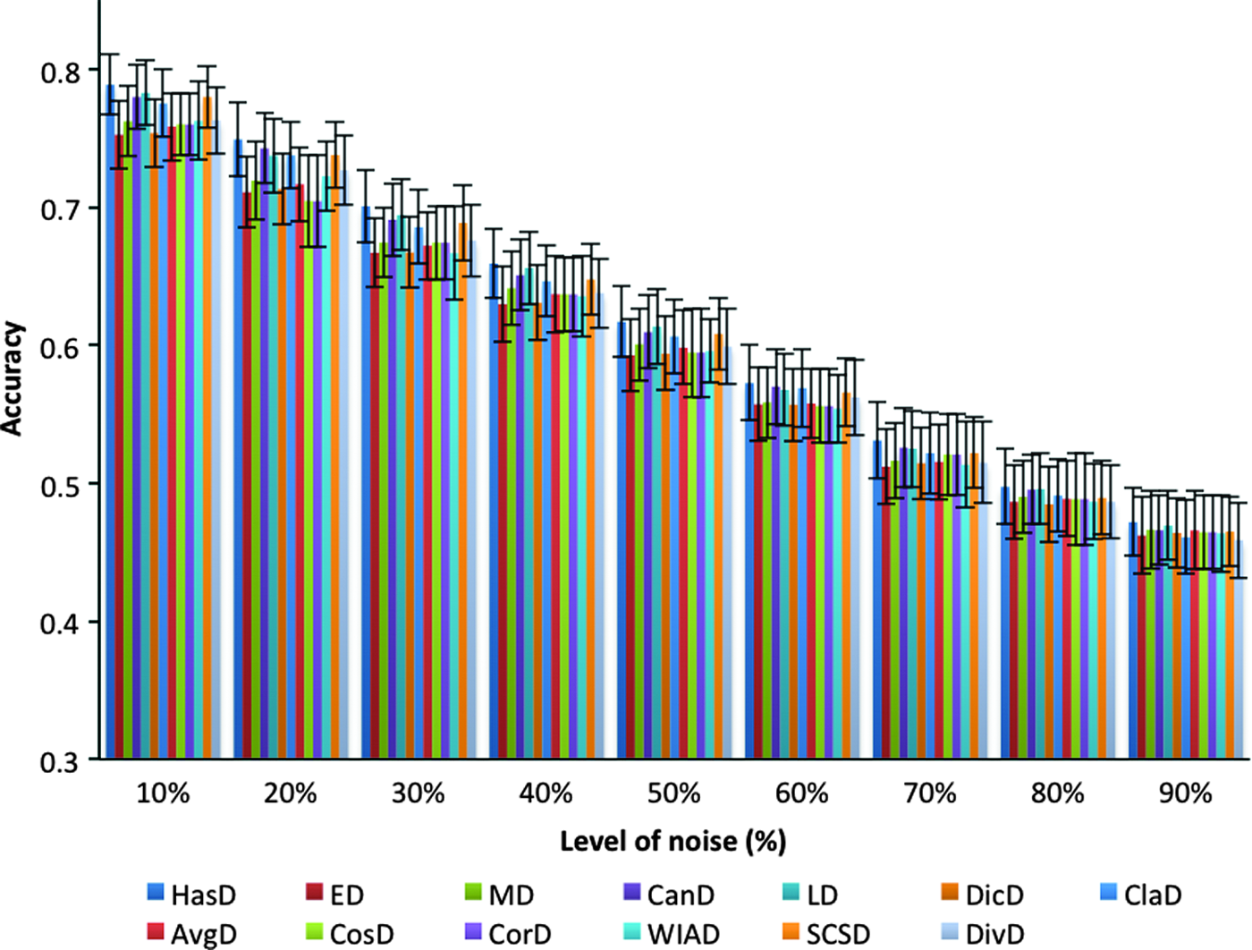
The overall average accuracies and standard deviations of KNN classifier using top 10 distance measures with different levels of noise. AvgD, Average (L₁, L_∞) distance; CanD, Canberra distance; ClaD, Clark distance; CorD, Correlation distance; CosD, Cosine distance; DicD, Dice distance; DivD, Divergence distance; LD, Lorentzian distance; MD, Manhattan distance; SCSD, Squared Chi-Squared; WIAD, Whittaker's index of association distance. Color images are available online.

FIG. 5.

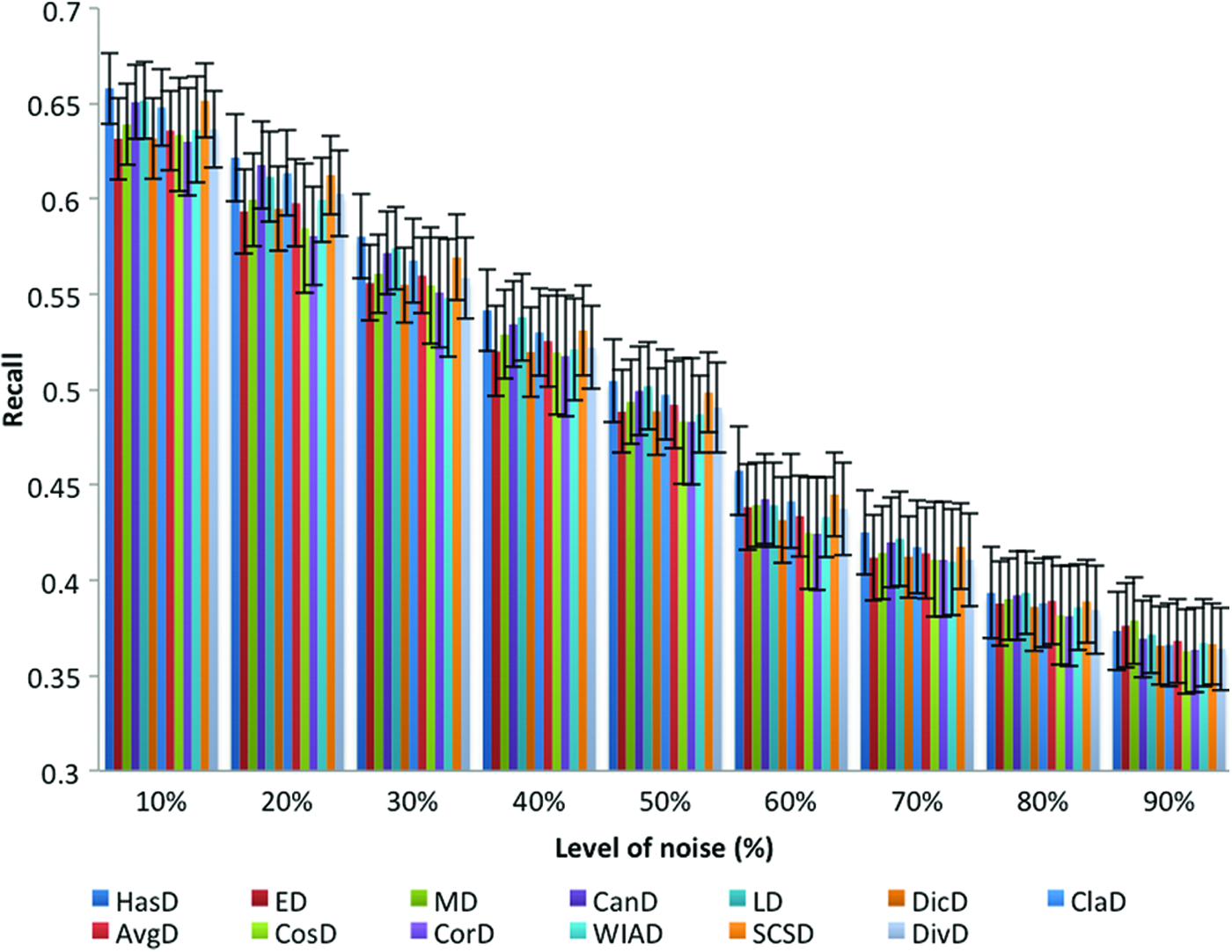
The overall average recalls and standard deviations of KNN classifier using top 10 distance measures with different levels of noise. Color images are available online.

FIG. 6.

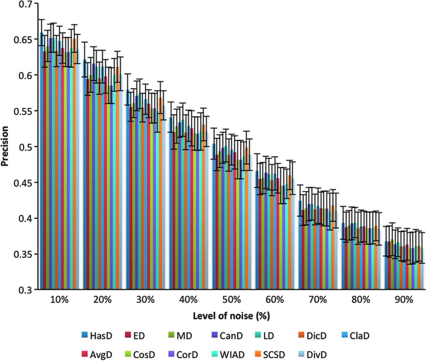
The overall average precisions and standard deviations of KNN classifier using top 10 distance measures with different levels of noise. Color images are available online.

Table 12.

Ranking of distances in descending order based on the accuracy results at each noise level

Rank	10%	20%	30%	40%	50%	60%	70%	80%	90%
1	HasD	HasD	HasD	HasD	HasD	HasD	HasD	HasD	HasD
2	LD	CanD	LD	LD	LD	CanD	CanD	LD	LD
3	CanD	SCSD	CanD	CanD	CanD	ClaD	LD	CanD	MD
	SCSD
4	ClaD	ClaD	SCSD	SCSD	SCSD	LD	SCSD	ClaD	CanD
5	DivD	LD	ClaD	ClaD	ClaD	SCSD	ClaD	MD	AvgD
6	WIAD	DivD	DivD	MD	MD	DivD	CosD	SCSD	SCSD
							CorD
7	MD	WIAD	MD	DivD	DivD	MD	MD	AvgD	CorD
			CosD
			CorD
8	CD	MD	AvgD	AvgD	AvgD	AvgD	AvgD	CorD	CosD
9	CorD	AvgD	DicD	CosD	WIAD	ED	DivD	CosD	DicD
				CorD
10	AvgD	DicD	ED	WIAD	CoD	DicD	DicD	DivD	WIAD
								WIAD
								ED
11	DicD	ED	WIAD	DicD	CorD	CorD	WIAD	DicD	ED
						CosD
12	ED	CosD	—	ED	DicD	WIAD	ED	—	ClaD
13	—	CorD	—	—	ED	—	—	—	DivD

Table 13.

Ranking of distances in descending order based on the recall results at each noise level

Rank	10%	20%	30%	40%	50%	60%	70%	80%	90%
1	HasD	HasD	HasD	HasD	HasD	HasD	HasD	LD, HasD	MD
2	LD	CanD	LD	LD	LD	SCSD	LD	CanD	ED
3	SCSD	ClaD	CanD	CanD	CanD	CanD	CanD	MD	HasD
4	CanD, SCSD	SCSD	SCSD	SCSD	ClaD	SCSD	AvgD	LD
5	ClaD	LD	ClaD	ClaD	ClaD	MD	ClaD	SCSD	CanD
6	MD	DivD	MD	MD	MD	LD	MD	ClaD	AvgD
7	DivD	MD	AvgD	AvgD	AvgD	ED	AvgD	ED	WIAD
8	WIOD	WIOD	DivD	DivD	DivD	DivD	DicD	DicD	SCSD
9	AvgD	AvgD	ED	WIAD	DicD	AvgD	ED	WIAD	ClaD
10	CosD	DicD	DicD	ED	ED	WIAD	CosD	DivD	DicD
							CorD
							DivD
11	DicD	ED	CosD	DicD	WIAD	DicD	WIAD	CosD	DivD
12	ED	CosD, CorD	CosD	CoD	CosD	—	CorD	CorD
13	CorD	CorD	WIOD	CorD	CorD	CorD	—	—	CosD

Table 14.

Ranking of distances in descending order based on the precision results at each noise level

Rank	10%	20%	30%	40%	50%	60%	70%	80%	90%
1	HasD	HasD	HasD	HasD	HasD	HasD	HasD	LD	MD
2	LD	CanD	LD	LD	LD	CanD	LD	HasD	HasD
3	CanD	ClaD	CanD	CanD	SCSD	ClaD	CanD	CanD	ED
4	SCSD	LD	SCSD	SCSD	CanD	LD	SCSD	MD	LD
		SCSD
5	ClaD	DivD	ClaD	ClaD	ClaD	SCSD	ClaD	SCSD	CanD
6	MD	MD	MD	MD	MD	MD	AvgD	ClaD	AvgD
			WIAD
7	AvgD	AvgD	AvgD	AvgD	AvgD	DivD	MD	AvgD	WIAD
8	WIAD	DicD	DivD	WIAD	ED	AvgD	CosD	ED	SCSD
							CorD
9	DivD	ED	ED	DivD	DivD	ED	DicD	CosD	DicD
								WIAD
10	DicD	CosD	DicD	ED	DicD	DicD	ED	CorD	ClaD
11	ED	CorD	CosD	DicD	WIAD	WIAD	DivD	DicD	DivD
			CorD
12	CosD	—	WIAD	CosD	CorD	CorD	WIAD	DivD	CorD
13	CorD	—	—	CorD	CosD	CosD	—	—	CosD

According to the average precision results, the highest precision was obtained by HasD, which achieved the first rank in the majority of noise levels. This distance succeeds to be in the first rank at noise levels 10% up to 70%. However, at a level 80%, LD outperformed HasD. Also, MD outperformed HasD at a noise level 90%.

LD achieved the second rank at noise levels 10%, 30%, 40%, 50%, and 70%. CanD achieved the second rank at noise levels 20% and 60%. Moreover, this distance achieved the third rank in the rest noise levels except at noise levels 50% and 90%. SCSD achieved the fourth rank at noise levels 10%, 30%, 40%, and 70%, and the third rank at a level of noise 50%. This distance was equal with LD at a noise level 20%. ClaD achieved the third rank at noise levels 20%, and 60%.

The rest of distances achieved the middle and the last ranks in different orders at each level of noise. CosD at level 80% was equal to WIAD in the result. This distance was also equal to CorD at levels 30% and 70%. These two distances performed the worst (lowest precision) in most noise levels.

Based on results given in Tables 12–14, we observe that the ranking of distances in terms of accuracy, recall, and precision without the presence of noise is different from their ranking when adding the first level of noise 10%, and it significantly varies when we increased the level of noise progressively. This means that the distances are affected by noise. However, the crucial question is, which one of the distances is least affected by noise? From the given results, we conclude that HasD is the least affected one, followed by LD, CanD, and SCSD. Good performance of the KNN achieved by these distances might be contributed by their good characteristics. Table 15 gives these characteristics of the top 10 distances in our analysis. All of these top 10 distances are symmetric, and we further provide input and output ranges and the number of operations.

Table 15.

Some characteristics of the top 10 distances (n is the number of features)

Distance	Input range	Output range	Symmetric	Metric	No. of operations
HasD	(−∞, +∞)	[0, n]	Yes	Yes	6n (positives), 9n (negatives)
ED	(−∞, +∞)	[0, +∞)	Yes	Yes	1 + 3n
MD	(−∞, +∞)	[0, +∞)	Yes	Yes	3n
CanD	(−∞, +∞)	[0, n]	Yes	Yes	7n
LD	(−∞, +∞)	[0, +∞)	Yes	Yes	5n
CosD	[0, +∞)	[0, 1]	Yes	No	5 + 6n
DicD	[0, +∞)	[0, 1]	Yes	No	4 + 6n
ClaD	[0, +∞)	[0, n]	Yes	Yes	1 + 6n
SCSD	(−∞, +∞)	[0, +∞)	Yes	Yes	6n
WIAD	(−∞, +∞)	[0, 1]	Yes	Yes	1 + 7n
CorD	[0, +∞)	[0, 1]	Yes	No	8 + 10n
AvgD	(−∞, +∞)	[0, +∞)	Yes	Yes	2 + 6n
DivD	(−∞, +∞)	[0, +∞)	Yes	Yes	1 + 6n

Precise evaluation of the effects of noise

To justify why some distances are affected either less or more by noise, the following toy Examples 1 and 2 are designed. These illustrate the effect of noise on the final decision of the KNN classifier using HasD and the standard ED. In both examples, we assume that we have two training vectors (v1 and v2) having three attributes for each, in addition to one test vector (v3). As usual, we calculate the distances between v3 and both v1 and v2 using both of ED and HasD.

Example 1. This example shows the KNN classification using two different distances on clean data (without noise). We find the distance to test vector (v3) according to ED and HasD.

	X1	X2	X3	X4	Class	Dist(⋅,V3)
	X1	X2	X3	X4	Class	ED	HasD
V1	3	4	5	3	2	2	0.87
V2	1	3	4	2	1	1	0.33
V3	2	3	4	2	?

As shown, assuming that we use k = 1, based on the 1-NN approach, and using both distances, the test vector is assigned to class 1, both results are reasonable, because V3 is almost the same as V2 (class = 1) except for the first feature, which differs only by 1.

Example 2. This example shows the same feature vectors as in Example 1, but after corrupting one of the features with an added noise. That is, we make the same previous calculations using noisy data instead of the clean data; the first attribute in V2 is corrupted by an added noise of (4, i.e., X1 = 5).

	X1	X2	X3	X4	Class	Dist(⋅,V3)
	X1	X2	X3	X4	Class	ED	HasD
V1	3	4	5	3	2	2	0.87
V2	5	3	4	2	1	3	0.5
V3	2	3	4	2	?

Based on the minimum distance approach, using Euclidian distance, the test vector is assigned to class 2 instead of 1. However, the test vector is assigned to class 1 using the HasD, this makes the distance more accurate with the existence of noise. Although simple, these examples showed that the ED was affected by noise and consequently affected the KNN classification ability. Although the performance of the KNN classifier is decreased as the noise increased (as shown by the extensive experiments with various data sets), we find that some distances are less affected by noise than other distances. For example, when using ED, any change in any attribute contributes highly to the final distance, even if both vectors were similar, but in one feature there was noise, the distance (in such a case) becomes unpredictable. In contrast, with the HasD we found that the distance between both consecutive attributes is bounded in the range [0,1], thus, regardless of the value of the added noise, each feature will contribute up to 1 maximally to the final distance, and not proportional to the value of the added noise. Therefore, the impact of noise on the final classification is mitigated.

It is worth mentioning that the aforementioned experiments used the KNN classifier with K equal to 1, also known as the nearest neighbor classifier. In fact, the choice of distance metric might affect the optimal K as well. A K = 1 choice is more sensitive to noise than larger K values, because an unrelated noisy example might be the nearest to a test example. Therefore, a valid action with noisy data would be to choose a larger K; it would be of interest to see which distance measure handles this aspect best. We remark that choosing the optimal K is out of the scope of this review, and we refer to Hassanat¹⁷ and Alkasassbeh et al.²⁵ However, we have repeated the experiments on all data sets using K = 3 and $k = \sqrt{n}$ , as done by Hassanat,¹⁷ where n is the number of examples in the training data set, with 50% noise. This is done using the top 10 distances. As given in Table 16, the average accuracy of most of the top 10 distances has been slightly improved compared with those shown in Figure 4 with noisy data, and Table 10 without noise, this is due to the larger number of neighbors (K) used; however, there are some exceptions, including the WIAD distance, which seems to be negatively affected by increasing the number of neighbors (K).

Table 16.

The average accuracy of the top 10 distances over all data sets, using K = 3 and $K = \sqrt{n}$ (n is the number of features), with and without noise

Distance	With 50% noise		Without noise
Distance	K = 3	$K = \sqrt{n}$	K = 3	$K = \sqrt{n}$
HasD	0.6302	0.6314	0.8497	0.833721
LD	0.6283	0.6237	0.8427	0.827561
CanD	0.6247	0.6231	0.8384	0.825171
ClaD	0.6171	0.6136	0.8283	0.8098
SCSD	0.6146	0.6087	0.8332	0.8045
MD	0.6124	0.6089	0.8152	0.79705
DivD	0.6114	0.6049	0.8183	0.792768
CosD	0.6086	0.6021	0.8085	0.791625
CorD	0.6085	0.6020	0.8085	0.786696
AvgD	0.6079	0.6081	0.8119	0.792768
ED	0.6016	0.6011	0.8031	0.781639
DicD	0.5998	0.6016	0.8021	0.778054
WIAD	0.5680	0.5989	0.7935	0.788361

In previous experiments, the noisy data have been used with the top 10 distances only. However, it would be interesting to see whether any of the other measures would handle noise better than these particular top 10 measures. Table 17 gives the average accuracy of all distances over the first 14 data sets, using K = 1 with and without noise. As given in Table 17, some of the top 10 distances still remain ranked the highest even with the existence of noise compared with all other distances, this includes HasD, LD, DivD, CanD, ClaD, and SCSD. However, interestingly, some of the other distances (which were ranked low when using data without noise) have shown less vulnerability to noise, these include SquD, PSCSD, MSCSD, SCD, MatD, and HeD. According to the extensive experiments conducted for the purpose of this review, and regardless of the type of the experiments, in general, the nonconvex distance HasD is the best distance to be used with the KNN classifier, with other distances such as LD, DivD, CanD, ClaD, and SCSD performing close to best.

Table 17.

The average accuracy of all distances over the first 14 data sets, using K = 1 with and without noise

Distance	With 50% noise	Without noise
HasD	0.6331	0.8108
LD	0.6302	0.7975
DivD	0.6284	0.8068
CanD	0.6271	0.8053
ClaD	0.6245	0.7999
SquD	0.6227	0.7971
PSCSD	0.6227	0.7971
SCSD	0.6227	0.7971
MSCSD	0.6223	0.8004
SCD	0.6208	0.7989
MatD	0.6208	0.7989
HeD	0.6208	0.7989
VSDF3	0.6179	0.7891
WIAD	0.6144	0.7877
CorD	0.6119	0.7635
SPeaD	0.6119	0.7635
CosD	0.6118	0.7636
NCSD	0.6108	0.7674
ChoD	0.6102	0.755
JeD	0.6071	0.7772
PCSD	0.6043	0.7813
KJD	0.6038	0.7465
PeaD	0.6034	0.7066
VSDF2	0.6032	0.7473
MD	0.6029	0.7565
NID	0.6029	0.7565
MCD	0.6029	0.7565
SD	0.6024	0.7557
SoD	0.6024	0.7557
MotD	0.6024	0.7557
ASCSD	0.6016	0.7458
VSDF1	0.6012	0.7427
AvgD	0.5995	0.7523
TanD	0.5986	0.7421
JDD	0.5955	0.741
MiSCSD	0.595	0.7596
VWHD	0.5945	0.7428
JacD	0.5936	0.746
DicD	0.5936	0.746
ED	0.5927	0.7429
SED	0.5927	0.7429
AD	0.5927	0.7429
KD	0.5911	0.7154
MCED	0.5889	0.7416
HamD	0.5843	0.7048
CD	0.5742	0.7154
HauD	0.5474	0.621
KDD	0.5295	0.5357
TopD	0.5277	0.6768
JSD	0.5276	0.6768
CSSD	0.5273	0.4895
KLD	0.5089	0.5399
MeeD	0.4958	0.4324
BD	0.4747	0.4908

Conclusions and Future Perspectives

In this review, the performance (accuracy, precision, and recall) of the KNN classifier has been evaluated using a large number of distance measures, on clean and noisy data sets, attempting to find the most appropriate distance measure that can be used with the KNN in general. In addition, we tried finding the most appropriate and robust distance that can be used in the case of noisy data. A large number of experiments conducted for the purposes of this review and the results and analysis of these experiments show the following:

The performance of KNN classifier depends significantly on the distance used, the results showed large gaps between the performances of different distances. For example, we found that HasD performed the best when applied on most data sets comparing with the other tested distances.

We get similar classification results when we use distances from the same family having almost the same equation, some distances are very similar, for example, one is twice the other, or one is the square of another. In these cases, and since the KNN compares examples using the same distance, the nearest neighbors will be the same if all distances were multiplied or divided by the same constant.

There was no optimal distance metric that can be used for all types of data sets, as the results show that each data set favors a specific distance metric, and this result complies with the no-free-lunch theorem.

The performance (measured by accuracy, precision, and recall) of the KNN degraded only ∼20% while the noise level reaches 90%, this is true for all the distances used. This means that the KNN classifier using any of the top 10 distances tolerates noise to a certain degree.

Some distances are less affected by the added noise comparing with other distances, for example, we found that HasD performed the best when applied on most data sets under different levels of heavy noise.

Our study has the following limitations, and future work will focus on studying, evaluating, and investigating these.

Although we have tested a large number of distance measures, there are still other distances and similarity measures that are available in the machine learning area that need to be tested and evaluated for optimal performance with and without noise.

The 28 data sets although higher than previously tested still might not be enough to draw significant conclusions in terms of the effectiveness of certain distance measures and, therefore, there is a need to use a larger number of data sets with varied data types.

The creation of noisy data is done by replacing a certain percentage (in the range 10%–90%) of the examples by completely random values in the attributes. We used this type of noise for its simplicity and straightforwardness in the interpretation of the effects of distance measure choice with KNN classifier. However, this type of noise might not simulate other types of noise that occur in the real-world data. It is an interesting task to try other realistic noise types to evaluate the distance measures for robustness in a similar manner.

Only KNN classifier was reviewed in this study, other variants of KNN such as Hassanat^90–93 need to be investigated.

Distance measures are not used only with the KNN, but also with other machine learning algorithms, such as different types of clustering, those need to be evaluated under different distance measures.

Footnotes

Author Disclosure Statement

No competing financial interests exist.

Abbreviations Used

References

Fix

, Hodges Jr

. Discriminatory analysis-nonparametric discrimination: Consistency properties. Technical report, University of California, Berkeley, 1951.

Cover

, Hart

. Nearest neighbor pattern classification. IEEE Trans Inf Theory. 1967; 13:21–27.

, Kumar

, Quinlan

, et al. Top 10 algorithms in data mining. Knowl Inf Syst. 2008; 14:1–37.

Bhatia

, Vandana

. Survey of nearest neighbor techniques. Int J Comput Sci Inf Secur. 2010; 8:302–305.

, Wu

. An algorithm for remote sensing image classification based on artificial immune b-cell network. ISPRS Arch. 2008; 37:107–112.

Manne

, Kotha

, Fatima

. Text categorization with K-nearest neighbor approach. In: Proceedings of the International Conference on Information Systems Design and Intelligent Applications, 2012 (INDIA 2012) held in Visakhapatnam, India, Springer, January 2012. pp. 413–420.

Geng

, Liu

T-Y

, Qin

, et al. Query dependent ranking using K-nearest neighbor. In: Proceedings of the 31st Annual International ACM SIGIR Conference on Research and Development in Information Retrieval, ACM, 2008. pp. 115–122.

Bajramovic

, Mattern

, Butko

, et al. A comparison of nearest neighbor search algorithms for generic object recognition. In: Proceedings of the International Conference on Advanced Concepts for Intelligent Vision Systems, Springer, 2006. pp. 1186–1197.

Yang

, Ault

, Pierce

, et al. Improving text categorization methods for event tracking. In: Proceedings of the 23rd Annual International ACM SIGIR Conference on Research and Development in Information Retrieval, ACM, 2000. pp. 65–72.

10.

Kataria

, Singh

. A review of data classification using k-nearest neighbour algorithm. Int J Emerg Technol Adv Eng. 2013; 3:354–360.

11.

Wettschereck

, Aha

, Mohri

. A review and empirical evaluation of feature weighting methods for a class of lazy learning algorithms. Artif Intell Rev. 1997; 11:273–314.

12.

Maillo

, Triguero

, Herrera

. A mapreduce-based K-nearest neighbor approach for big data classification. In: 2015 IEEE Trustcom/BigDataSE/ISPA, Volume 2, IEEE, 2015. pp. 167–172.

13.

Maillo

, Ramírez

, Triguero

, et al.. KNN-is: An iterative spark-based design of the K-nearest neighbors classifier for big data. Knowl Based Syst. 2017; 117:3–15.

14.

Deng

, Zhu

, Cheng

, et al. Efficient KNN classification algorithm for big data. Neurocomputing. 2016; 195:143–148.

15.

Gallego

A-J

, Calvo-Zaragoza

, Valero-Mas

, et al. Clustering-based K-nearest neighbor classification for large-scale data with neural codes representation. Pattern Recogn. 2018; 74:531–543.

16.

Wang

, Wang

, Nie

, et al. Efficient tree classifiers for large scale datasets. Neurocomputing. 2018; 284:70–79.

17.

Hassanat

AB.

Solving the problem of the k parameter in the KNN classifier using an ensemble learning approach. Int J Comput Sci Inf Secur. 2014; 12:33–39.

18.

Chomboon

, Chujai

, Teerarassamee

, et al. An empirical study of distance metrics for K-nearest neighbor algorithm. In: Proceedings of the 3rd International Conference on Industrial Application Engineering. Kitakyushu, Japan: The Institute of Industrial Applications Engineers, 2005. pp. 1–6.

19.

Mulak

, Talhar

. Analysis of distance measures using K-nearest neighbor algorithm on KDD dataset. Int J Sci Res. 2015; 7:2101–2104.

20.

Tavallaee

, Bagheri

, Lu

, et al. A detailed analysis of the KDD cup 99 data set. In: 2009 IEEE Symposium on Computational Intelligence for Security and Defense Applications, IEEE, 2009. pp. 1–6.

21.

L-Y

, Huang

M-W

, Ke

S-W

, et al. The distance function effect on K-nearest neighbor classification for medical datasets. SpringerPlus. 2016; 5:1304.

22.

Todeschini

, Ballabio

, Consonni

. Distances and other dissimilarity measures in chemometrics. In: Meyers

(ed). Encyclopedia of Analytical Chemistry. Hoboken, NJ: Wiley Online Library, 2015.

23.

Todeschini

, Ballabio

, Consonni

, et al. A new concept of higher-order similarity and the role of distance/similarity measures in local classification methods. Chemom Intell Lab Syst. 2016; 157:50–57.

24.

Lopes

, Ribeiro

On the impact of distance metrics in instance-based learning algorithms. In: Iberian Conference on Pattern Recognition and Image Analysis, Springer, 2015. pp. 48–56.

25.

Alkasassbeh

, Altarawneh

, Hassanat

. On enhancing the performance of nearest neighbour classifiers using Hassanat distance metric. Can J Pure Appl Sci. 2015; 9:3291–3298.

26.

Hassanat

AB.

Dimensionality invariant similarity measure. J Am Sci. 2014; 10:221–226.

27.

Jirina

. Using singularity exponent in distance based classifier. In: 2010 10th International Conference on Intelligent Systems Design and Applications, IEEE, 2010. pp. 220–224.

28.

Lindi

GA.

Development of face recognition system for use on the NAO robot. Master's thesis, Faculty of Science and Technology, 2016.

29.

Jiřina

, Jiřina Jr

Classifier based on inverted indexes of neighbors. Technical Report No. V-1034, 2008.

30.

Abbadi

, Altarawneh

, Hassanat

, et al. Solving the problem of the k parameter in the KNN classifier using an ensemble learning approach. Int J Comput Sci Inf Secur. 2014; 12:33–39.

31.

Hart

. The condensed nearest neighbor rule (CORRESP.). IEEE Trans Inf Theory. 1968; 14:515–516.

32.

Gates

. The reduced nearest neighbor rule (CORRESP.). IEEE Trans Inf Theory. 1972; 18:431–433.

33.

Alpaydin

Voting over multiple condensed nearest neighbors. In: Lazy Learning, Springer, 1997. pp. 115–132.

34.

Kubat

, Cooperson, Jr

Voting nearest-neighbour subclassifiers. In: The 17th International Conference on Machine Learning (ICML), San Francisco, CA: Morgan Kaufmann, 2000. pp. 503–510.

35.

Wilson

, Martinez

. Reduction techniques for instance-based learning algorithms. Mach Learn. 2000; 38:257–286.

36.

Arya

, Mount

. Approximate nearest neighbor queries in fixed dimensions. SODA. 1993; 93:271–280.

37.

Zheng

, Guo

, Tung

AKH

, et al. Lazylsh: Approximate nearest neighbor search for multiple distance functions with a single index. In: Proceedings of the 2016 International Conference on Management of Data, ACM, 2016. pp. 2023–2037.

38.

Nettleton

, Orriols-Puig

, Fornells

. A study of the effect of different types of noise on the precision of supervised learning techniques. Artif Intell Rev. 2010; 33:275–306.

39.

Zhu

, Wu

. Class noise vs. attribute noise: A quantitative study. Artif Intell Rev. 2004; 22:177–210.

40.

García

, Luengo

, Herrera

. Data preprocessing in data mining. Cham, Switzerland: Springer International Publishing, 2015.

41.

SáEz

, Galar

, Luengo

, et al. Tackling the problem of classification with noisy data using multiple classifier systems: Analysis of the performance and robustness. Inf Sci. 2013; 247:1–20.

42.

Heath

TL.

The thirteen books of Euclid's Elements. North Chelmsford, MA: Courier Corporation, 1956.

43.

Cha

S-H.

Comprehensive survey on distance/similarity measures between probability density functions. City, 2007; 1:1.

44.

Deza

, Deza

Encyclopedia of distances. In: Encyclopedia of distances, Springer, 2009. pp. 1–583.

45.

Grabusts

The choice of metrics for clustering algorithms. In: Proceedings of the 8th International Scientific and Practical Conference, Volume 2. Tomsk, Russia: Tomsk Polytechnic University, 2011. pp. 70–76.

46.

Premaratne

Human computer interaction using hand gestures. Singapore: Springer Science and Business Media, 2014.

47.

Verma

JP.

Data analysis in management with SPSS software. New Delhi, India: Springer Science and Business Media, 2012.

48.

Lance

, Williams

. Computer programs for hierarchical polythetic classification (“similarity analyses”). Comput J. 1966; 9:60–64.

49.

Lance

, Williams

. Mixed-data classificatory programs I—agglomerative systems. Aust Comput J. 1967; 1:15–20.

50.

Akila

, Chandra

. Slope finder—A distance measure for DTW based isolated word speech recognition. Int J Eng Comput Sci. 2013; 2:3411–3417.

51.

Sorensen

TA.

A method of establishing groups of equal amplitude in plant sociology based on similarity of species content and its application to analyses of the vegetation on danish commons. Biol Skar. 1948; 5:1–34.

52.

Szmidt

Distances and similarities in intuitionistic fuzzy sets (Studies in Fuzziness and Soft Computing book series). Cham, Switzerland: Springer, 2014.

53.

Ngom

, Chetty

, Ahmad

. Pattern recognition in bioinformatics. Berlin, Heidelberg: Springer, 2008.

54.

Zhou

, Chan

KCC

, Wang

Topevm: Using co-occurrence and topology patterns of enzymes in metabolic networks to construct phylogenetic trees. In: IAPR International Conference on Pattern Recognition in Bioinformatics, Springer, 2008. pp. 225–236.

55.

Willett

, Barnard

, Downs

. Chemical similarity searching. J Chem Inf Comput Sci. 1998; 38:983–996.

56.

Jaccard

. Comparative study of the floral distribution in a portion of the Alps and Jura [in French]. Bull Soc Vaudoise Sci Nat. 1901; 37:547–579.

57.

Cesare

, Xiang

. Software similarity and classification. London, England: Springer Science and Business Media, 2012.

58.

Dice

LR.

Measures of the amount of ecologic association between species. Ecology. 1945; 26:297–302.

59.

Gan

, Ma

, Wu

. Data clustering: Theory, algorithms, and applications (ASA-SIAM Series on Statistics and Applied Probability), volume 20. Philadelphia, PA: Society for Industrial and Applied Mathematics, 2007.

60.

Orloci

An agglomerative method for classification of plant communities. J Ecol. 1967; 55:193–206.

61.

Legendre

, Legendre

LFJ

. Numerical ecology, volume 24. Amsterdam, Netherlands: Elsevier, 2012.

62.

Shirkhorshidi

, Aghabozorgi

, Wah

. A comparison study on similarity and dissimilarity measures in clustering continuous data. PLoS One. 2015; 10: e0144059.

63.

Bhattacharyya

On a measure of divergence between two statistical populations defined by their probability distributions. Bull Calcutta Math Soc. 1943; 35:99–109.

64.

Abbad

, Tairi

. Combining Jaccard and Mahalanobis cosine distance to enhance the face recognition rate. Int J Eng Comput Sci. 2016; 16:171–178.

65.

Hellinger

New justification of the theory of quadratic forms of infinite variables [in German]. J Reine Angew Math. 1909; 136:210–271.

66.

Clark

PJ.

An extension of the coefficient of divergence for use with multiple characters. Copeia. 1952; 1952:61–64.

67.

Neyman

Contributions to the theory of the χ² test. In: Proceedings of the first Berkeley Symposium on Mathematical Statistics and Probability. University of California Press, Berkeley, 1949.

68.

Pearson

X. on the criterion that a given system of deviations from the probable in the case of a correlated system of variables is such that it can be reasonably supposed to have arisen from random sampling. London Edin Dubl Phil Mag J Sci. 1900; 50:157–175.

69.

Shannon

CE.

A mathematical theory of communication. ACM SIGMOBILE Mobile Comput Commun Rev. 2001; 5:3–55.

70.

Kullback

, Leibler

. On information and sufficiency. Ann Math Stat. 1951; 22:79–86.

71.

Pinto

, Benedí

J-M

, Rosso

Clustering narrow-domain short texts by using the Kullback-Leibler distance. In: International Conference on Intelligent Text Processing and Computational Linguistics, Springer, 2007. pp. 611–622.

72.

Jeffreys

An invariant form for the prior probability in estimation problems. Proc R Soc London Ser A Math Phys Sci. 1946; 186:453–461.

73.

Topsoe

Some inequalities for information divergence and related measures of discrimination. IEEE Trans Inf Theory. 2000; 46:1602–1609.

74.

Sibson

Information radius. Information radius [in German]. Prob Theory Rel. 1969; 14:149–160.

75.

Hatzigiorgaki

, Skodras

. Compressed domain image retrieval: A comparative study of similarity metrics. In: Visual Communications and Image Processing 2003, volume 5150, International Society for Optics and Photonics, 2003. pp. 439–448.

76.

Patel

, Meshram

. Content based video retrieval systems. arXiv preprint arXiv:1205.1641, 2012.

77.

Giusti

, Batista

GEAPA

. An empirical comparison of dissimilarity measures for time series classification. In: 2013 Brazilian Conference on Intelligent Systems, IEEE, 2013. pp. 82–88.

78.

Macklem

Multidimensional modelling of image fidelity measures. Centre County, PA: Citeseer, 2002.

79.

Bharkad

, Kokare

. Performance evaluation of distance metrics: Application to fingerprint recognition. Int J Pattern Recogn. 2011; 25:777–806.

80.

Hedges

TS.

An empirical modification to linear wave theory. Proc Inst Civ Eng. 1976; 61:575–579.

81.

Taneja

IJ.

New developments in generalized information measures. Adv Imag Elect Phys. 1995; 91:37–135.

82.

Fulekar

MH.

Bioinformatics: Applications in life and environmental sciences. Dordrecht, Netherlands: Springer Science and Business Media, 2009.

83.

Hamming

RW.

Error detecting and error correcting codes. Bell Syst Tech J. 1950; 29:147–160.

84.

Kadir

, Nugroho

, Susanto

, et al. Experiments of distance measurements in a foliage plant retrieval system. Int J Signal Process Image Process Pattern Recogn. 2012; 5:1–14.

85.

Rubner

, Tomasi

. Perceptual metrics for image database navigation, volume 594. New York, NY: Springer Science and Business Media, 2013.

86.

Whittaker

RH.

A study of summer foliage insect communities in the great smoky mountains. Ecol Monogr. 1952; 22:1–44.

87.

UC Irvine. 2016. UC Irvine machine learning repository. Available online at http://archive.ics.uci.edu/ml (last accessed July 10, 2019).

88.

Wilcoxon

Individual comparisons by ranking methods. In: Kotz

, Johnson

(eds): Breakthroughs in statistics. New York, NY: Springer, 1992. pp. 196–202.

89.

Derrac

, García

, Molina

, et al. A practical tutorial on the use of nonparametric statistical tests as a methodology for comparing evolutionary and swarm intelligence algorithms. Swarm Evol Comput. 2011; 1:3–18.

90.

Hassanat

ABA.

Two-point-based binary search trees for accelerating big data classification using KNN. PLoS One. 2018; 13: e0207772.

91.

Hassanat

Furthest-pair-based decision trees: Experimental results on big data classification. Information. 2018; 9:284.

92.

Hassanat

ABA.

Furthest-pair-based binary search tree for speeding big data classification using K-nearest neighbors. Big Data. 2018; 6:225–235.

93.

Hassanat

Norm-based binary search trees for speeding up KNN big data classification. Computers. 2018; 7:54.