NSVD : Normalized Singular Value Deviation Reveals Number of Latent Factors in Tensor Decomposition

Abstract

Tensor decomposition has been shown, time and time again, to be an effective tool in multiaspect data mining, especially in exploratory applications where the interest is in discovering hidden interpretable structure from the data. In such exploratory applications, the number of such hidden structures is of utmost importance since incorrect selection may imply the discovery of noisy artifacts that do not really represent a meaningful pattern. Although extremely important, selection of this number of latent factors, also known as low-rank, is very hard, and in most cases, practitioners and researchers resort to ad hoc trial-and-error or assume that somehow this number is known or is given via domain expertise. There has been a considerable amount of prior work that proposes heuristics for selecting this low rank. However, as we argue in this article, the state of the art in those heuristic methods is rather unstable and does not always reveal the correct answer. In this article, we propose the Normalized Singular Value Deviation (NSVD), a novel method for selecting the number of latent factors in Tensor Decomposition that is based on principled theoretical foundations. We extensively evaluate the effectiveness of NSVD in synthetic and real data and demonstrate that it yields a more robust, stable, and reliable estimation than state of the art. Finally, we provide an efficient compression scheme for facilitating the use of NSVD in very big tensors.

Introduction

Data analysis and pattern extraction have always been an important tool in science and everyday life since they provide a fundamental way of understanding, organizing, and solving problems that may arise. In fact, these problems are often characterized by a multidimensional profile, which in turn can produce an explosion in the complexity of the problem, and, thus, create a temptation to resort toward simplified and biased solutions that are easier to figure out.

It is becoming increasingly apparent, however, that finding ways to tackle these issues in their original multiaspect form can provide answers of superior quality and unmatched insight.^1,2 Therefore, it makes sense to search for methods that can encapsulate this characteristic in a way simple enough that will also enable us to make useful discoveries about the task at hand. Tensors, which have traditionally been a mathematical tool, offer exactly this capability since they possess the simplicity of a multidimensional array and hence are able to capture the multiple facets of the problem at hand. Albert Einstein's general relativity, which was formulated using tensors, is a particularly interesting example that demonstrates their power. At the same time, a broad range of interesting results in tensors^3,4 provides an elegant mathematical framework, which allows us to derive important and insightful conclusions about the nature of the tensor data and their structure.

PARAFAC decomposition^5,6 and Kruskal's uniqueness conditions⁴ have laid out an important part of the foundation for using multidimensional arrays as a tool for multiaspect data mining. PARAFAC decompositions express the data as the sum of other elementary rank one tensors, and when performed properly, they can reveal a lot about the underlying structure of the data. However, finding the right number of components for a PARAFAC decomposition is not an easy task. To make this more clear, consider tensor rank, which is another important concept^7–9 and is closely tied to finding a proper number of components for a PARAFAC decomposition. Tensor rank calculation has been proven to be NP-Hard over $ℚ$ ^9,10 and over any extension of it including $ℝ$ and $ℂ$ , and NP-Complete over finite fields.¹¹ Therefore, it becomes understood that despite the solid mathematical foundations that have been set so far, we are still a long way from finding a broadly efficient solution that sufficiently tackles this problem.

For this reason, people have resorted to heuristic ways for discovering low-rank structure in data,^12–14 and even though some of them might enjoy success in specific domains, they are usually unable to generalize robustly to a broader spectrum of applications. In this work, we are exploring some of these pathways, and we are suggesting a different way of looking at this problem. Our contributions are:

A novel low-rank structure detection method: We propose a new technique for finding the appropriate number of PARAFAC components, by performing a simple but powerful transformation to the decomposition, which enables us the use of important linear algebra tools.

Extensive theoretical analysis: We provide and prove various advantageous theoretical properties of our technique, while pointing out the respective shortcomings in the theoretical formulation of an existing widely used method.

Thorough experimental evaluation: Multiple experiments for various settings are carried out on real and artificial data, to study and evaluate the behavior of our method in comparison to other baselines.

A well-behaved compression scheme for big tensors: An efficient type of tensor compression is examined with the aim of speeding up calculations for big data tensors, without compromising the effectiveness of our method.

Reproducibility: To promote reproducibility of our results, we make our code for NSVD and the synthetic tensor generator used in the article publicly available.^*

Problem Formulation

Notation and definitions

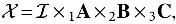
Even though tensors are often defined as elements of specific tensor product spaces that correspond to multilinear maps, it is common in the field of data mining to define an N-mode tensor as an element of the tensor product of N arbitrary vector spaces. Similar to matrices, if we choose a basis for each vector space, then the tensor can be represented as a multidimensional array of numbers. Without loss of generality, in this work, we will study only three-mode tensors , where I, J, and K are the dimensions of the respective vector spaces.

Additionally, along with Table 1, we have the following definitions:

Table 1.

Table of symbols

Symbol	Definition
x	Scalar
$X$	Matrix
	Tensor
	Kronecker product
	Column-wise Khatri–Rao product
	Outer product

Mode-n Fiber: A column vector produced by fixing the indices in all the dimensions of the tensor except from the n-th dimension. For example, the Mode-1 fibers of a $2 \times 2 \times 2$ tensor can be identified as for all $j, k = 1, 2$ .

n-Mode Product: It is denoted as , where $M$ is an $L \times I_{n}$ matrix and I_n is the n-th dimension of . It modifies by transforming its mode-n fibers as .

Frobenius Norm: .

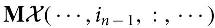Vectorization: It is denoted as vec and is a column vector constructed by concatenating all mode-1 fibers , with the smaller j and k having higher priority in the concatenation, and similarly, the second dimension has higher priority than the third dimension.

PARAFAC decomposition

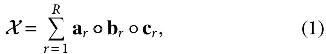
As already discussed, tensor decompositions play an important role in discovering structure in multiaspect data. Even though a plethora of decompositions have been proposed, in this work, we will only concern ourselves with the PARAFAC decomposition since it has a very close connection to the rank of a tensor . To see this, we first express in terms of its PARAFAC decomposition as follows:

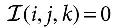where $A \in ℝ^{I \times R}$ , $B \in ℝ^{J \times R}$ , and $C \in ℝ^{K \times R}$ are the PARAFAC factor matrices, R is the number of PARAFAC components, also called CP-rank, and for which it holds that if $i = j = k$ and otherwise. Note that this expression can be reformulated as

where $a_{r}$ , $b_{r}$ , and $c_{r}$ are the r-th columns of the factor matrices $A$ , $B$ , and $C$ , respectively. Since this is the sum of R rank one tensors, it becomes evident that if we manage to find the minimum R for which Equation (1) holds, then we have essentially found the rank of the tensor. Additionally, for fixed values of R, the PARAFAC decomposition is usually approximated by using alternating least squares algorithms,^5,6 which minimize the Frobenius norm of the error.

An important obstacle in finding the optimal R though is the fact that even for a CP-rank less than the actual tensor rank, there is the possibility that a decomposition exists that produces an arbitrarily small error. This can occur due to the fact that a rank-R best approximation of a tensor might not even exist.¹⁵ Thus, a common and intuitive idea is to calculate approximate PARAFAC decompositions for a range of CP-ranks and then evaluate them with an effective diagnostic tool that will hopefully uncover the decomposition with the proper number of components.

AutoTen and the Core Consistency Diagnostic

As already discussed, rank estimation and low-rank trilinear structure discovery are very difficult problems, and there are currently no general purpose tools that can efficiently accomplish these tasks. It is worth elaborating, however, on some of the most effective tools, two of which are AutoTen¹⁶ and the Core Consistency Diagnostic (CORCONDIA).^12,17

AutoTen is a tool that aims to provide unsupervised detection of multilinear low-rank structure in tensors and is currently considered the state of the art among its competitors who also attempt to automate the task. In closer inspection, however, one can observe that AutoTen's success can in large part be attributed to the power of CORCONDIA, which is one of its main building blocks, and, therefore, for all intents and purposes, we can directly study and analyze the behavior of CORCONDIA instead of AutoTen's.

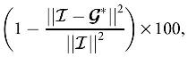
To make this claim concrete, we first remind that given the PARAFAC factor matrices $A$ , $B$ , and $C$ of , CORCONDIA is defined as

where

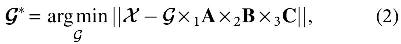
or equivalently

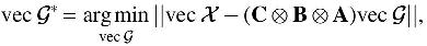
which shows that the calculation of corresponds to a linear least squares problem.

Essentially, CORCONDIA evaluates how well a PARAFAC decomposition captures low-rank trilinear structure in the data by comparing it to how well the data are modeled when interactions among the components of the decomposition are allowed. These interactions are described by the off-diagonal elements of , and therefore, we see that when a lot of them have nonzero values, then CORCONDIA will tend to have large values. Notice that for in Equation (2) not only there exist no interactions between the components, but this is exactly how PARAFAC is formulated in the least squares sense. Since CORCONDIA attains its goal by comparing with $ℐ$ , when their difference is small, CORCONDIA will have a value close to 100, which implies that the corresponding decomposition is appropriate and captures mostly trilinear structure in the data. However, if the difference is not trivial, CORCONDIA can get close to zero or even negative, which is a strong indication that the given decomposition is not capturing properly the trilinear variation in the data, and hence, it should probably be discarded.

Since there could be multiple models, which give a high value of CORCONDIA, the way that we choose between them is by selecting the one that also has the largest number of components. The reason that we choose this model is because it will most probably also provide the best fit in terms of the squared norm of the error. In this manner, we can explore a trade-off between the quality of the model based on CORCONDIA and its fit.

Based on this reasoning, AutoTen attempts to produce accurate estimates of the real number of components by examining CORCONDIA at CP-ranks where it starts dropping from 100 to 0. AutoTen calculates CORCONDIA in the least squares sense but is generally able to generate finer estimates by further considering CORCONDIA based on the Kullback–Leibler divergence. In this work, we will focus on the least squares based CORCONDIA, and below, we elaborate on some of its drawbacks, which can have a serious impact on the performance of AutoTen.

One of the weaknesses of CORCONDIA stems from the fact that even with a unique PAFAFAC decomposition, the factor matrices still suffer from scaling and permutation indeterminacies. To make this clear, consider the R-component PARAFAC of and the resulting from Equation (2). Note also that an equally valid set of factor matrices would be $A P S_{A}$ , $B P S_{B}$ , and $C P S_{C}$ , where $P$ is a permutation matrix and $S_{A}$ , $S_{B}$ , and $S_{C}$ are diagonal scaling matrices for which it holds that $S_{A} S_{B} S_{C} = I$ . In this case, Equation (2) would give

where . This is minimized only if

Therefore, there is an infinite number of valid , which in turn implies that CORCONDIA will not have a unique value.

Proposed Method: NSVD

Since CORCONDIA can suffer from such indeterminacies, which can create instabilities in the quality of its estimates, we propose a new method for discovering trilinear structure in tensor data and mitigating the issue above. Our method also possesses additional useful properties that provide further support for its power and robustness, as discussed in the following subsections.

Theoretical formulation

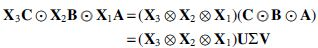
The first and probably the most important observation that we have to make is that the Khatri–Rao product is a matrix, which has the vectorized factors of the decomposition as its columns. This transformation is critical for our analysis since it allows us to manipulate and make inferences about the quality and the properties of a PARAFAC decomposition by employing a plethora of very well-established tools in linear algebra.

Specifically, notice that we can use the singular values of as a proxy for the behavior of any PARAFAC decomposition. This is a particularly interesting choice as explained in the following lemmas.

Lemma 1. The singular values of are unaffected by the scaling and permutation indeterminacies of PARAFAC.

Proof. Scaling issues are directly solved by the Khatri–Rao product as

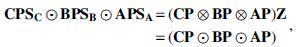
where is exactly the matrix that can transform the Kronecker product to the Khatri–Rao product when multiplied from the right.¹⁸

Regarding the permutation indeterminacy, first, we observe that performing identical column permutations on A, B, and C and then computing their Khatri–Rao product produces the same result as when we first calculate their Khatri–Rao product and then we perform the same column permutations on this matrix. This is the same as saying that , which in turn means that if the Singular Value Decomposition (SVD) of is , then the SVD of can be calculated as with and thus consists of the same singular values. ▪

Notice that these singular values can capture the essence of the decomposition in just a few parameters. This can prove a crucial factor in evaluating the decompositions since using other quantities such as the norm of the error, , involves a huge number of parameters, which can lead to greater inaccuracies. A specific example of this idea is presented experimentally in the next section, where it becomes obvious that in various cases a method based on the norm of the error can indeed be inadequate, as opposed to a method based on the singular values of . In particular, for any R-component PARAFAC decomposition of , we only need to study R singular values, as opposed to an aggregation of the $I \cdot J \cdot K$ errors. Note that even though these singular values are also obtained based on all the elements of , they can provide a more stable means of evaluation since they also have nice properties as discussed in the lemmas below.

Lemma 2. The Kronecker product of any set of n matrices $A_{i}$ is an orthogonal matrix if, and only if, all $A_{i}$ are multiples of orthogonal matrices, such that $A_{i}^{T} A_{i} = c_{i} I$ and $\prod_{i = 1}^{n} c_{i} = 1$ .

See the Appendix for proof.

Lemma 3. The singular values of are identical, up to scaling, to the singular values produced by all tensors of the form $X \times_{1} R_{1} \times_{2} R_{2} \times_{3} R_{3}$ , for $R_{1}$ , $R_{2}$ , and $R_{3}$ multiples of arbitrary orthogonal matrices.

Proof. Considering again the SVD of , we observe that every other possible matrix of the same size that has the same singular values will have the form , where and are orthogonal matrices. However, not every orthogonal and results in a matrix that has the Khatri–Rao structure . Therefore, if we set and select a that is in the Kronecker form , then following Lemma 2, R₁, R₂, and R₃ have to be multiples of orthogonal matrices and the product of the norms of their corresponding columns has to be equal to one. However, observe that any multiple of is also a valid choice if we let the singular values absorb the scaling, that is, . ▪

In other words, these singular values can be viewed as a more direct identifier of the structure of without being as prone to changes in the actual form of the tensor. Particularly, this implies that although methods such as CORCONDIA or the norm of the error might report bad evaluations for orthogonal rotations of the decomposition, the singular values of will signify that the decomposition is appropriate since they will be identical, up to scaling, to the ones corresponding to the PARAFAC of the original unrotated .

The importance of this becomes more evident if we consider the fact that the set of tensors consisting of and all its orthogonal rotations contain in some sense the same underlying structure, even though directly looking at their elements on a high level might make them appear as completely different tensors. In fact, all these tensor representations correspond to the exact same abstract tensor in different bases, which imply that a sound rank estimation method should ideally produce similar rank estimates for all of them.

Additionally, it is not unreasonable to expect that multiple approximate solutions of an optimization algorithm for PARAFAC, produced by using different randomly generated initial points, for example, will generally be similar to each other when the specified number of components captures the underlying structure properly. However, we can expect the solutions to have greater deviations from each other when the given number of components cannot describe the structure of the data properly. Particularly, notice that for a fixed number of components, there could be a huge number of ways that extraneous components can be combined to produce the decomposition when we decompose with more components than necessary.

Based on this observation, we propose the use of the variances of the singular values of as a means to detecting and properly quantifying such deviations. Specifically, to provide fair comparisons, we divide these variances by the respective expected values, and, finally, we aggregate all these quantities by calculating the sum of their logarithms. Using the logarithm has a twofold advantage since it provides numerical stability and leads to more interpretable plots. Numerical inaccuracies can occur if we only consider the product of the variances of the singular values since individual variances sometimes take values very close to zero. Also, considering that different CP-ranks can lead to a change of many orders of magnitude to this product, we can see that the logarithm provides a more suitable option.

More formally, considering a probability distribution for the random initializations of the algorithm that calculates the R-component PARAFAC, and given the variance $σ_{R, i}^{2}$ and the expected value $μ_{R, i}$ of the i-th singular value of , we compute $\sum_{i = 1}^{R} log (σ_{R, i}^{2} ∕ μ_{R, i})$ , which we will call Normalized Singular Value Deviation (NSVD). In this manner, we are able to discover possible trilinear structure in the data and the number of PARAFAC components that best models it, with distinct dips in NSVD being an indication of more appropriate decompositions.

In summary, NSVD consists of the following steps:

Step 1: Compute multiple R-component PARAFAC decompositions by using multiple random initializations for the algorithm that calculates them.

Step 2: Form the Khatri–Rao product for each decomposition.

Step 3: Compute the singular values of each and estimate the variance $σ_{R, i}^{2}$ and the expected value $μ_{R, i}$ of the i-th singular value, for all $i = 1 \dots R .$

Step 4: Compute $f (R) = \sum_{i = 1}^{R} log (σ_{R, i}^{2} ∕ μ_{R, i})$ .

Step 5: Repeat Steps 1–4 for multiple values of R.

Step 6: Estimate that k number of PARAFAC components appropriately model the underlying structure of the data if $f (k)$ is the lowest part of a distinct dip.

Notice that we did not specify a method for calculating the optimal expected value and variance estimates since their optimality depends on their desired properties. However, to keep things simple and effective, in all our experiments, we are going to make use of the sample mean and the unbiased sample variance.

Compression

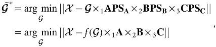
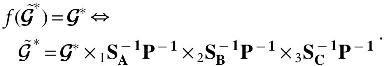
At this point, it is important to consider the fact that when we are dealing with big tensor data in practice, all these rank estimation methods might struggle to properly execute due to large memory and compute time requirements. For this reason, we propose the use of an efficient compression scheme,^19–21 which aims to mitigate these issues, and we also provide a sufficient theoretical condition in Lemma 4, which guarantees the robustness of NSVD when applied on the compressed data.

The compression scheme is as simple as multiplying mode-wise with three compressor matrices $X_{1} \in ℝ^{L \times I}$ , $X_{2} \in ℝ^{M \times J}$ , and $X_{3} \in ℝ^{N \times K}$ , such that $L ≪ I$ , $M ≪ J$ , and $N ≪ K$ . Therefore, we can efficiently calculate the compressed tensor $X_{c o m p} = X \times_{1} X_{1} \times_{2} X_{2} \times_{3} X_{3}$ , which contains only $L \cdot M \cdot N$ elements, thus enabling NSVD to discover low-rank trilinear structure in , by performing calculations on the much smaller $X_{c o m p}$ . Specifically, notice that in the cases where has an exact R-component PARAFAC decomposition such that $X = ℐ \times_{1} A \times_{2} B \times_{3} C$ , then we can easily derive an exact R-component PARAFAC decomposition for the compressed tensor as $X_{c o m p} = (ℐ \times_{1} A \times_{2} B \times_{3} C) \times_{1} X_{1} \times_{2} X_{2} \times_{3} X_{3} = ℐ \times_{1} X_{1} A \times_{2} X_{2} B \times_{3} X_{2} C$ , which gives the PARAFAC factor matrices $X_{1} A$ , $X_{2} B$ , and $X_{3} C$ . NSVD can now make use of the much smaller Khatri–Rao product instead and continue with its computations without demanding enormous amounts of resources.

Additionally, to ensure that NSVDs behavior will remain unaffected when applied on the compressed data, we can make the following lemma.

Lemma 4. The compressed tensor $X_{c o m p}$ produces the same singular values as the uncompressed tensor , if $L M N \geq R$ and the first LMN left singular vectors of transformed by form an orthonormal set of vectors.

Proof. Given the SVD of we have that

First, observe that , where 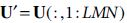and . Thus, according to our assumptions, we can see that the matrix 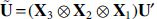will be orthogonal, which in turn implies that will be the SVD of 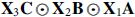. Finally, since we design the compressor matrices such that $L M N \geq R$ , and will have identical singular values.

Note that, even when the assumptions in the previous lemma are difficult to satisfy with certainty, NSVD can discover structure in practice by performing multiple random compressions using compressor matrices with orthonormal rows, as suggested in Ref.²¹ In the Discovering Structure in Compressed Tensors section, we experimentally verify the validity of this lemma for both real and artificial data.

Experimental Evaluation

In our experiments, at each number of components, R, we approximate NSVD by first calculating a number, K, of PARAFAC estimates using random initializations for the optimization algorithm. These PARAFACs are then used for the estimation of the necessary unbiased sample variances and sample means of the singular values of . Finally, we aggregate all these estimates as explained in the Theoretical Formulation section to get our NSVD estimate for R components.

For more accurate results, we calculate NSVD on the first k samples, and we repeat this for all k ranging from 2 to K. The final NSVD estimate is calculated based on these $K - 1$ intermediate estimates. Also, note that for the baselines, we use similar calculations. For further implementation details, we refer the interested reader to the Appendix.

Finally, Tensor Toolbox^22,23 was used for calculating all PARAFAC decompositions, and N-way Toolbox²⁴ was used only in cases where there exist missing data. Also, in all plots, the horizontal axis always represents the number of PARAFAC components, whereas the error bars signify the 25th and 75th percentiles of the $K - 1$ intermediate NSVD estimates. The error bars for the baselines are calculated in a similar manner.

Artificial data

A first step in evaluating our method is to assess its performance on artificially generated data whose structure can be defined explicitly. In the following experiments, we create artificial tensors by generating three matrices with R columns each, where their elements are drawn from the standard normal distribution. Note that if we consider these matrices as the PARAFAC factor matrices of our tensor, then the rank of the tensor will be at most R, since it will be the sum of R rank – 1 factors. Additionally, these factor matrices will be full column rank with very high probability, which in turn implies that the R factors will also be linearly independent. Therefore, the rank of the tensor will be exactly R.

To achieve a better approximation of real tensor data scenarios, however, our rank-R tensor, , is distorted by an additive noise tensor , which is a rank-100 tensor generated in the same way as but has its norm scaled to be p times less than the norm of . In other words, the final tensor will be 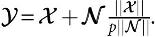In this manner, we generated the $20 \times 20 \times 20$ SynthSmall tensor having five components and $p = 2$ , which is studied in the Comparison to Baselines section. This procedure was also used to generate the $1 0^{5} \times 1 0^{5} \times 1 0^{5}$ SynthBig tensor again with five components and $p = 2$ , compressed versions of whom are studied in the Discovering Structure in Compressed Tensors section.

Also, keep in mind that although there is not a perfect way of generating artificial data, our method is attempting to provide good approximations of real tensor data, without losing the flexibility and robustness provided by its mathematical foundation. The data generator and the NSVD code are available online.^†

Real data

Even though NSVD behaves nicely on artificial tensor data, indicating a distinctive dip exactly where the predefined number of components is, it is important to also study its performance and behavior on real tensor data to assess its practicality in real-world scenarios. For this reason, we analyze a range of real data sets as shown in Table 2.

Table 2.

Tensors analyzed in the experimental section

Name	Dimensions	Components
Chem1	$351 \times 19 \times 83$	6 (Chem. Verified)
Chem2	$351 \times 18 \times 83$	5 (Chem. Verified)
Chem3	$351 \times 22 \times 83$	5 (Chem. Verified)
Reality Mining	$94 \times 94 \times 4$	6 (see Ref.²⁸)
Enron	$184 \times 184 \times 44$	4 and 7 (see Ref.^31,32)
SynthSmall	$20 \times 20 \times 20$	5 (Synthetic)
SynthBig	$1 0^{5} \times 1 0^{5} \times 1 0^{5}$	5 (Synthetic)

Chemical data

First, we analyze the chemical data sets Chem1, Chem2, and Chem3. These data sets are a small time interval taken from a large tensor data set where 44 wine samples were measured on a gas chromatographic system with mass spectrometry detection. Each interval represents a subset on the time axis where a few specific chemical compounds appear. The aim of modeling the data is to separate the overlapping signals from the compounds. One additional chemical data set of this type is studied in the Appendix.

Note that data of this nature have generally been observed to have a strong trilinear structure. Therefore, when we are called to discover the individual chemical substances in the chemical samples, performing decompositions such as PARAFAC and identifying the proper number of components become tasks of central importance. Moreover, many times it is possible to chemically identify the number of components in the samples. Therefore, these useful properties render chemical data a very attractive tool for the evaluation of methods such as ours, which aim to provide estimations for the rank of a tensor or detect low-rank multilinear structure in data. Unfortunately, however, the chemical data studied in this work have not become publicly available, which limits our ability to meaningfully study and explain their various components.

Social network data

It is understood that arbitrary real-world data do not necessarily possess a strict notion of structure that can be accurately translated to mathematical concepts such as tensor rank and PARAFAC decomposition. However, this incompatibility is not necessarily due to an inherent weakness in tensor-based structure discovering methods. On the contrary, the problem many times lies in that it can be very difficult to give an exact definition of what constitutes structure in complicated data like this. Nevertheless, as we will see, tensor-based methods have proven to be very effective in uncovering structure even in these scenarios, and for this reason in our work, we also study two additional nonchemical real data sets.

First, we study the Reality Mining data set,²⁵ which includes data gathered by the MIT Media Laboratory in the context of an experiment assessing the behavior of social communities. These communities consist of 100 subjects who participated in the study, 94 of which are included in our data set. The experiment was conducted by special software that was installed in the phones of the participants, and among others, it recorded four distinct communication aspects for each subject, that is, calls, Bluetooth devices nearby, text messages, and friendship with the rest of the subjects, which form a three-mode tensor with four slices. Various studies have been conducted on this data set,^26,27 and particularly in Ref.,²⁸ the authors discovered and elaborated on six dominant communities.

We are also evaluating our method on the famous Enron data set, which was made public after the corporation's scandal was uncovered. The data set contains a large number of e-mails that were exchanged between around 150 employees of the company and has attracted a lot of attention,^29,30 mainly due to the fact that it probably is the only publicly available large-scale data set of real-world e-mails. In our work, we study a smaller version of the data set obtained as explained in Ref.,³¹ which consists of the communication between 184 e-mail addresses in an interval of 44 weeks, and, therefore, can be represented as a three-mode tensor. In the same study, the authors identified and elaborated on four distinct communities, whereas in Ref.,³² the authors, after running multiple iterations of their experiments, claimed to have discovered a total of seven communities with a standard deviation of 0.88.

Comparison to baselines

Detecting structure in data can be a daunting task, especially when one attempts to automate the process and make it as universally and domain agnostic as possible. Many heuristic methods have been proposed for this purpose,^12–14 each with its own advantages and drawbacks, often making it necessary to resort to different structure finding techniques depending on the problem at hand.

It is crucial for the evaluation of NSVD, therefore, to put it into the test against other baselines and in turn assess its capability in revealing the correct number of components for a range of artificial and real data sets. The comparison is carried out on the data described in the Artificial Data section and the Real Data section using 100 iterations for the calculation of all NSVD estimates, except for the Reality Mining data set where 74 iterations were used due to limitations in computational resources. The following baselines are considered in the comparison:

CORCONDIA: (see the AutoTen and the Core Consistency Diagnostic section)

Squared Error (SE): It is defined as the squared frobenious norm of the difference between the original tensor and its approximation. We then estimate that R components best describe the trilinear variation in the data if the R-component PARAFAC gives a low enough SE compared with PARAFACs with different number of components. This usually manifests as a distinct dip at R components.

SE on missing data: Similar to the usual SE, with the only difference being that the PARAFAC decompositions are estimated using only the known data of the tensor, and the SE is calculated on the missing data. Note that if R components produce low SE on the missing data, it can be interpreted as that the corresponding PARAFAC model can better predict them, and, hence, we can estimate that an R-component underlying structure is appropriate. In our work, we always assume $20 %$ of missing data selected randomly in each iteration.

Synthetic data

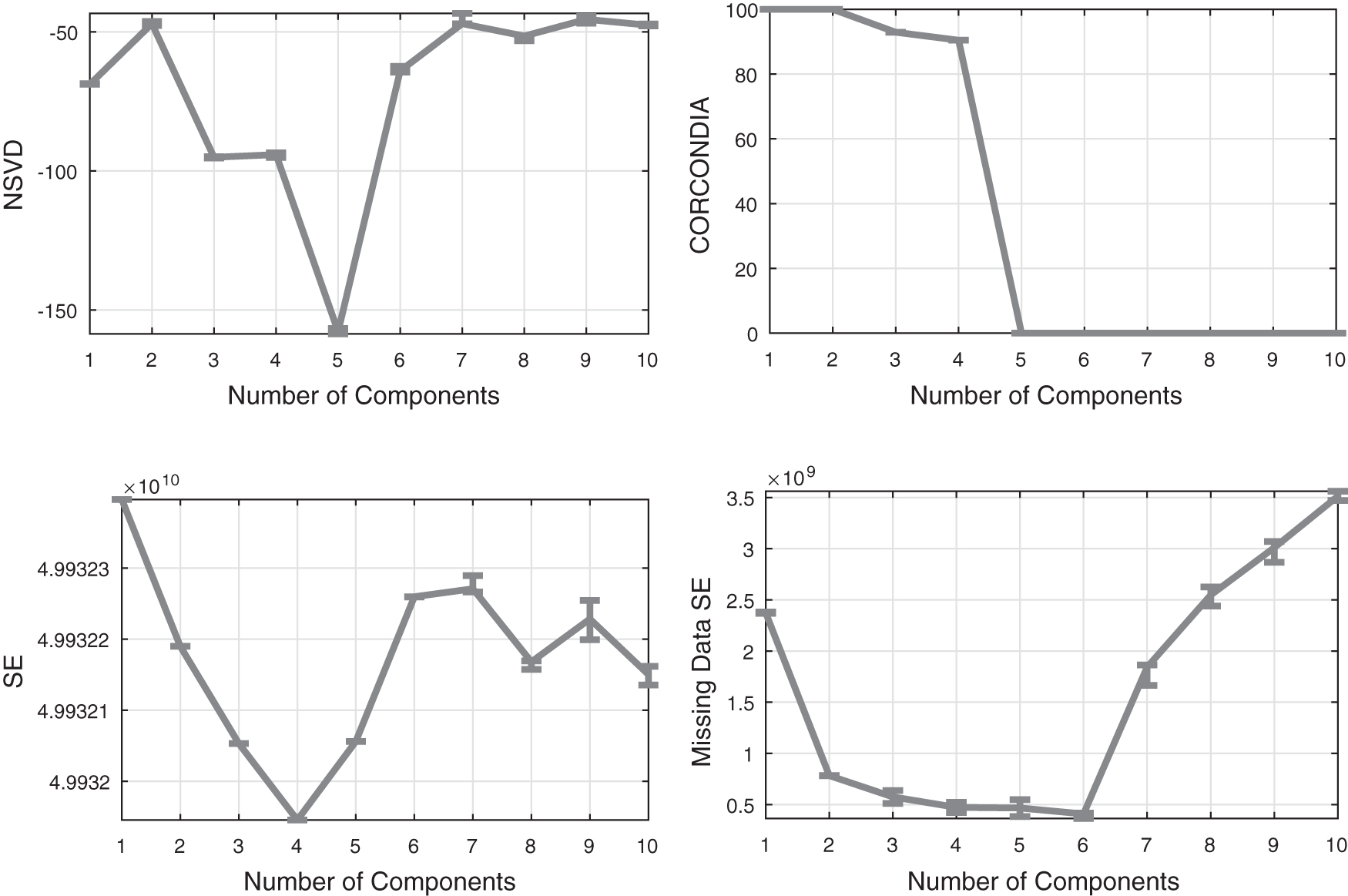
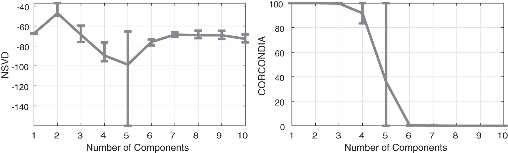
For our synthetic data set SynthSmall, we observe in Figure 1 that NSVD presents a quite distinct dip at five components, which is the correct answer. However, even though CORCONDIA seems to approximate a region around five components, it struggles to give a definitive answer and leaves open the possibility of up to seven or even eight components. Interestingly, even SE seems to be working better than CORCONDIA in this case, showing a subtle indication at five components, which get amplified when using SE on the missing data.

FIG. 1.

Baselines comparison on the SynthSmall data set.

Chemical data

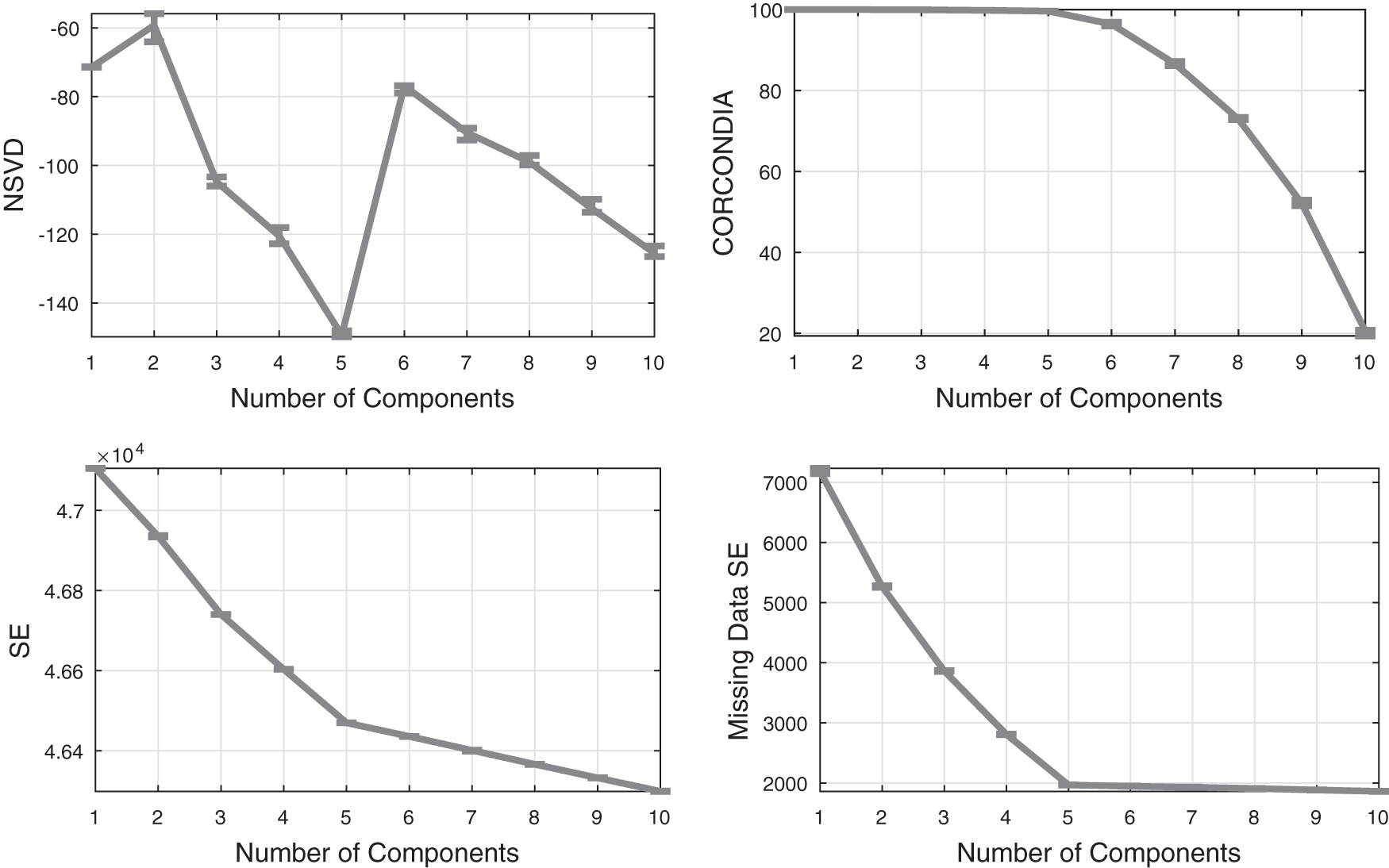
In Figure 2, we can see the nice indication that NSVD provides for the six components of Chem1, as opposed to CORCONDIA, which suggests only three components. SE also fails to identify the correct answer by vaguely indicating only four or five components, and similarly for the SE on missing data, which suggest only four components.

FIG. 2.

Baselines comparison on the Chem1 data set.

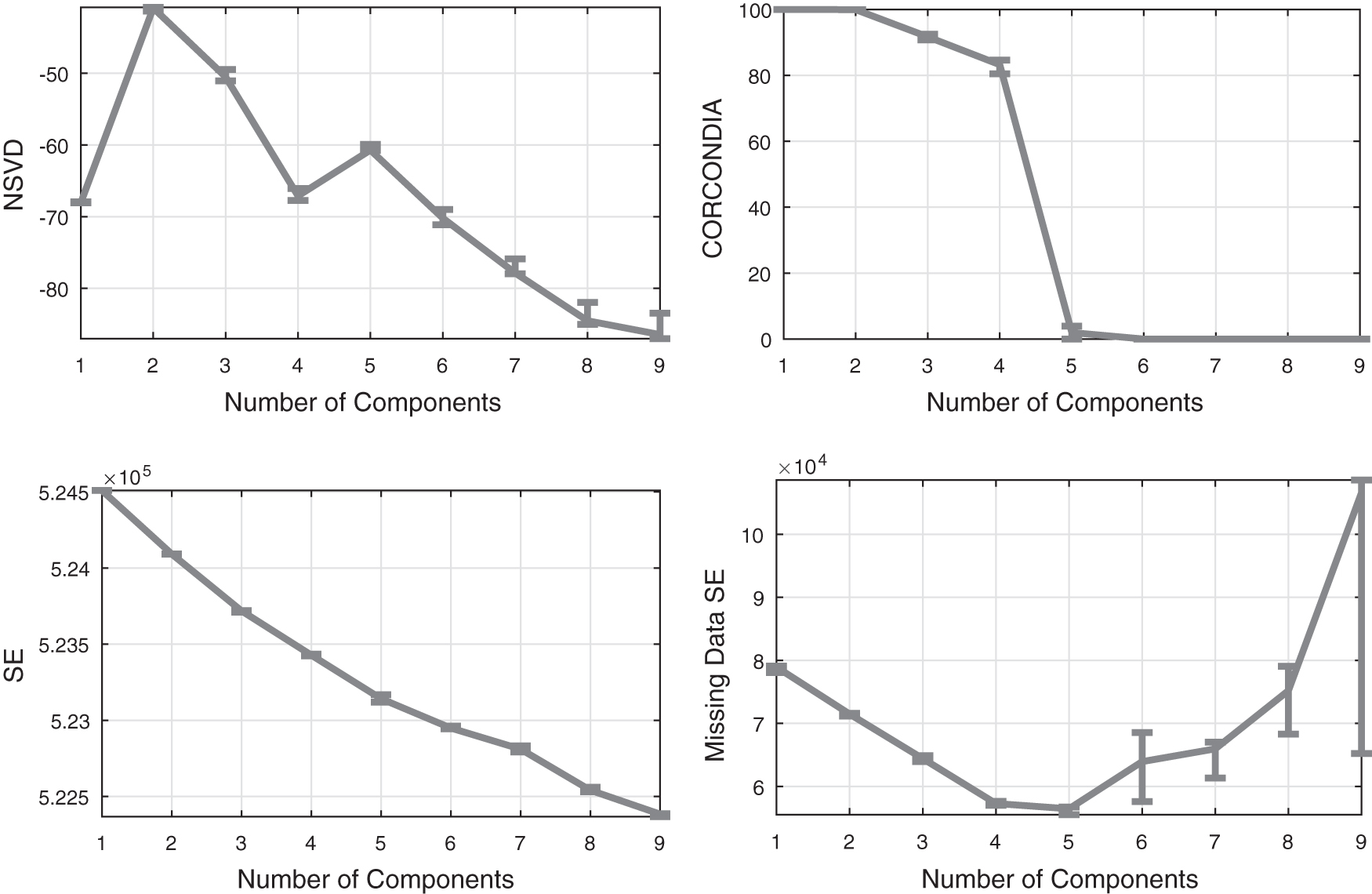
The situation is different for Chem2 where all baselines fail to discover the five components in the data, as shown in Figure 3. CORCONDIA provides a vague estimate of around three components, whereas SE shows a distinct dip also at three components. SE on missing data also fails to give a definitive answer, even though it slightly hints at four components. However, NSVD provides a much clearer indication at four and five components, and although it is not as sharp as in the previous examples, it outperforms all the baselines.

FIG. 3.

Baselines comparison on the Chem2 data set.

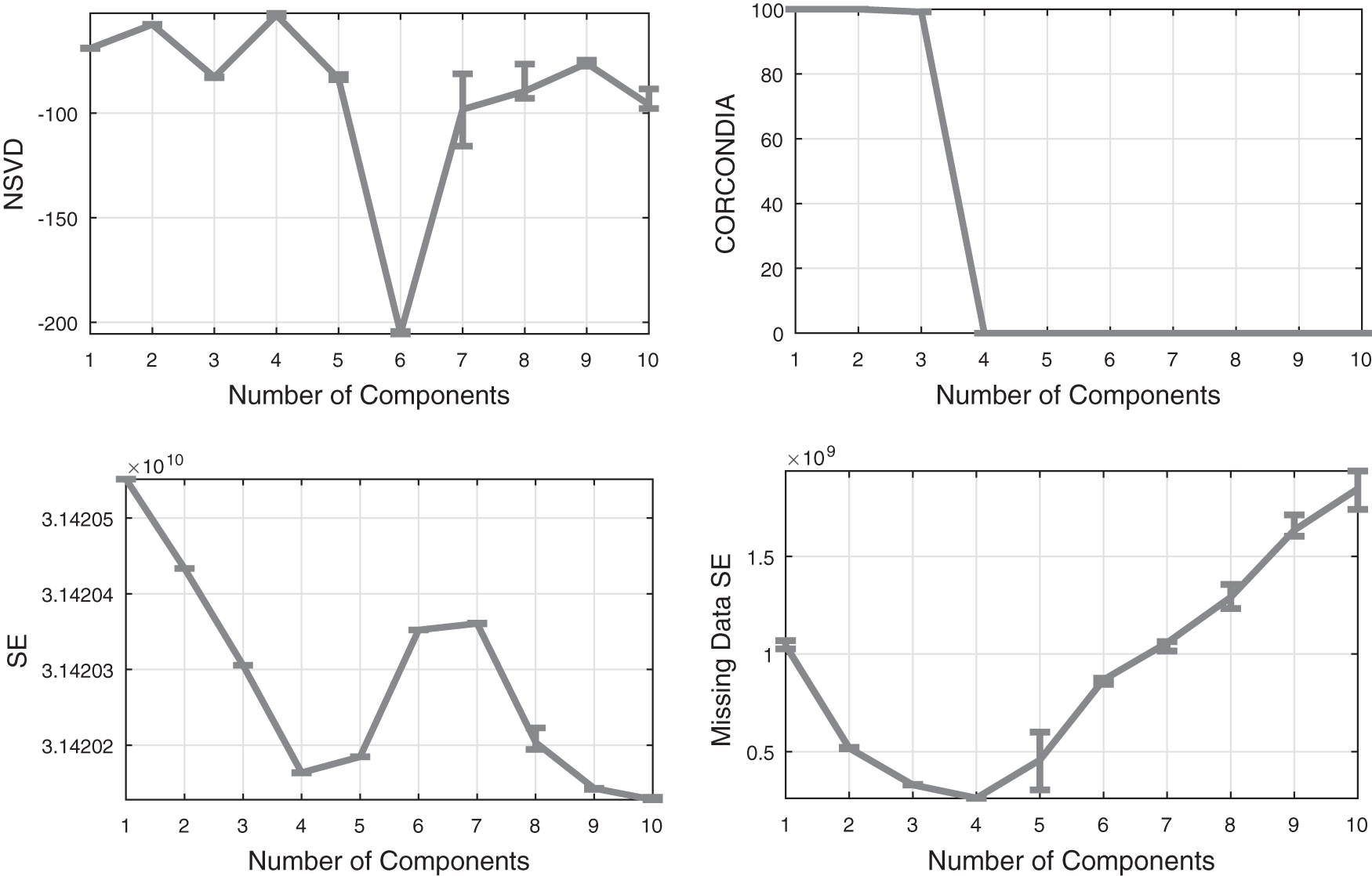
Chem3 in Figure 4 gives another interesting example where NSVD triumphs once again over the baselines by clearly detecting the five components in the data. CORCONDIA and SE, however, even though they provide a clear estimate of four components, they fail to provide any hint for five components. Furthermore, even though SE on missing data provides indication for three to six components that include the correct answer, it contains no clear evidence for choosing five components instead of the rest of the options.

FIG. 4.

Baselines comparison on the Chem3 data set.

Social network data

In Figure 5, we see that the behavior of NSVD on the Reality Mining data set is more convoluted, providing multiple indications at three, six, and nine components. CORCONDIA provides an indication only at three components, whereas SE hints at three and six components. Note that even though it is hard to obtain ground truth for this type of data, NSVD is able to at least suggest potential structure at all the points where both CORCONDIA and SE do as well. It is also interesting to observe that the six components that the authors identified in Ref.²⁸ make sense considering that not only both NSVD and SE provide an indication at this number of components but also SE takes its lowest value at that point too. Finally, SE on missing data fails to provide a clear estimate since it could indicate anything from one to four components.

FIG. 5.

Baselines comparison on the Reality Mining data set.

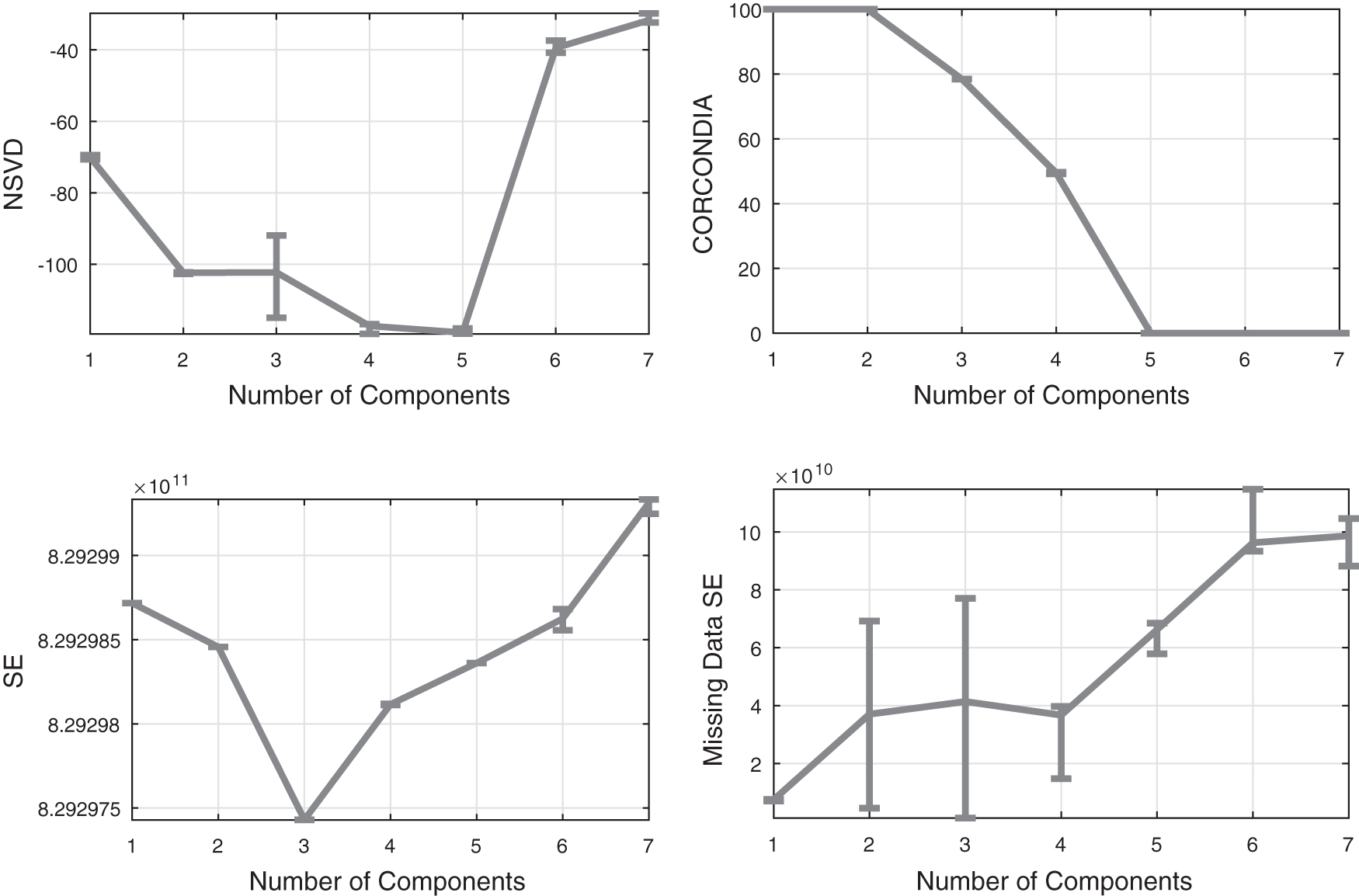
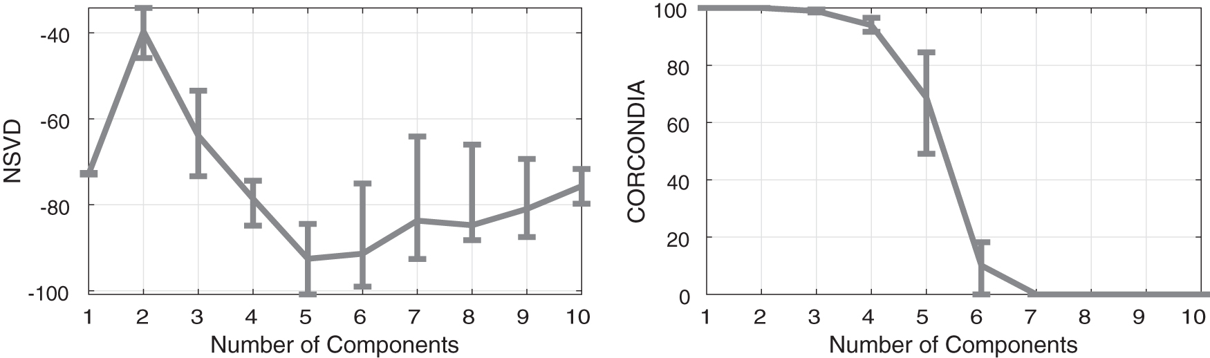
Last, we have the Enron data set in Figure 6 where NSVD successfully identifies four components as suggested in Ref.³¹ CORCONDIA is the only baseline that also manages to provide a sharp and correct estimate, whereas the SE is showing no indication at any number of components. However, SE on missing data is able to perform somewhat better by indicating a not very sharp estimate of four or five components. In the Fine-Tuning NSVD section, we also show that under proper tuning, NSVD is capable of identifying six and seven components, which are compatible with the estimation provided in Ref.³²

FIG. 6.

Baselines comparison on the Enron data set.

Fine-tuning NSVD

At this point, we are going to demonstrate an interesting property of NSVD, which makes it even more flexible and versatile, allowing it to provide sharper and more accurate estimates, and even uncover different levels of structure in the data. Additionally, this improvement can be achieved by only fine-tuning a simple parameter; the tolerance for the termination criterion of the optimization algorithm that calculates the PARAFAC decompositions.

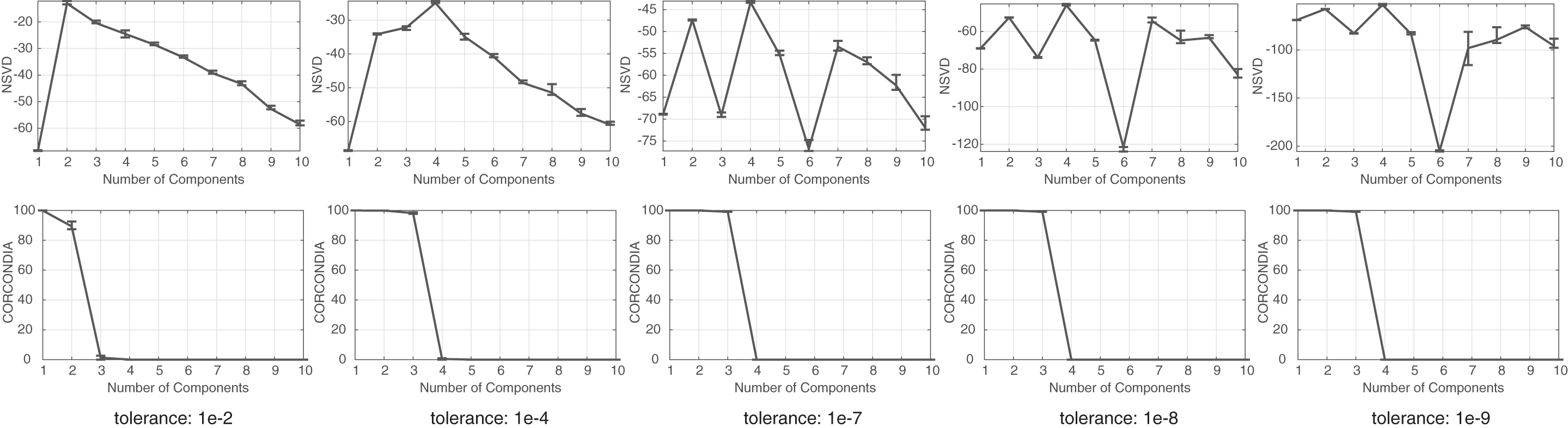
Specifically, in Figure 7, we calculate NSVD and CORCONDIA on Chem1 for tighter tolerances from the left to right, and we observe that NSVD begins showing indications of structure for a tolerance of $1 e - 7$ at three and six components. Making the tolerance even tighter and equal to $1 e - 8$ and $1 e - 9$ , results in similar estimates, but with the correct estimate of six components being incrementally more pronounced. However, we observe that in all cases, CORCONDIA only manages to identify three components, which are of course in disagreement with the given ground truth of six components for Chem1.

FIG. 7.

NSVD and CORCONDIA on the Chem1 data set for tighter tolerances from the left to right. Observe how NSVD is able to provide finer and more pronounced estimates by fine-tuning the tolerance level. CORCONDIA, Core Consistency Diagnostic; NSVD, Normalized Singular Value Deviation. For ease of reading, the figure can be viewed online.

We can make an even more impressive observation in Figure 8 where NSVD is tested on the Enron data set for multiple tolerance levels. At first, for the low tolerance of $1 e - 2$ , NSVD provides no robust estimate at all. However, at a tolerance of $1 e - 3$ , it shows a distinct indication at four components, which are in agreement with the findings in Ref.³¹ Next, for a tolerance of $7 e - 4$ , we see that NSVD starts transitioning from an estimate of four to an estimate of six components, which later become the only pronounced estimate for a tolerance of $1 e - 4$ and $1 e - 7$ . In the end, NSVD seems to stabilize at seven components for the even tighter tolerances of $1 e - 10$ and $1 e - 12$ . Notice that the last estimates of six and seven components are in perfect agreement with the findings in Ref.,³² where seven components were identified with a standard deviation of 0.88. However, CORCONDIA is able to only discover four components and remains virtually unaffected by the changes in the tolerance levels, except for a tolerance of $7 e - 4$ where its estimate gets distorted.

FIG. 8.

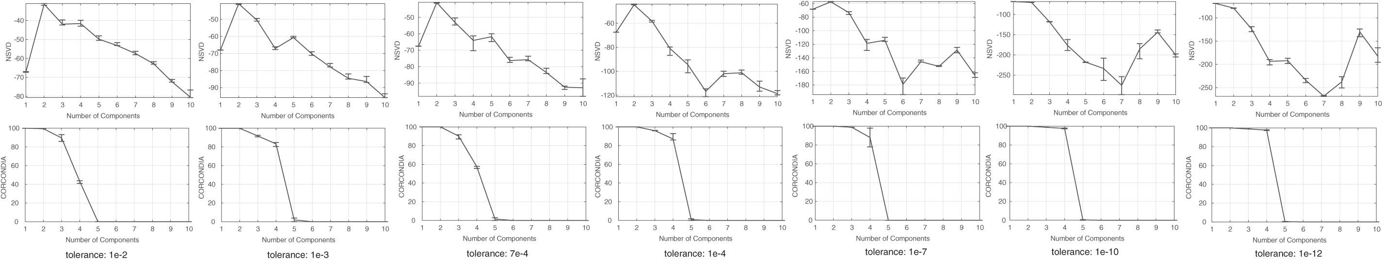
NSVD and CORCONDIA on the Enron data set for tighter tolerances from the left to right. Observe how NSVD is able to reveal multiple structures in the data by using different tolerances. For ease of reading, the figure can be viewed online.

Discovering structure in compressed tensors

As we already mentioned in the Compression section, compression can be a critical step in making NSVD a lot more efficient when dealing with big tensor data. Since it is usually difficult to guarantee that compression will not distort the structure of a tensor significantly, we will take the approach of calculating multiple random compressions using orthonormal matrices. Note that we will quantify compression levels by a percentage that signifies how much each mode is shrinked. For example, using a compression of $80 %$ on a $100 \times 100 \times 100$ tensor gives a compressed tensor of size $80 \times 80 \times 80$ .

In Figures 9 and 10, we study the performance of NSVD on the SynthBig tensor for compressions of $0.1 %$ and $0.01 %$ , which shrink its size from $1 0^{5} \times 1 0^{5} \times 1 0^{5}$ to $100 \times 100 \times 100$ and $10 \times 10 \times 10$ , respectively. In both cases, a tolerance of $1 e - 6$ was used and 800 PARAFACs of the compressed tensor were calculated, while substituting each compression with a new one every 50 iterations. Remember that this artificial tensor was designed to have five components, and the norm of the noise was set as high as 50% of the norm of the data. Also, in this case, we calculate the intermediate samples on each compressed tensor individually, and then, we calculate the final estimates and the 25th and 75th percentiles by considering collectively all these samples of all compressed tensors.

FIG. 9.

NSVD and CORCONDIA on compressions of the SynthBig tensor of size $100 \times 100 \times 100$ .

FIG. 10.

NSVD and CORCONDIA on compressions of the SynthBig tensor of size $10 \times 10 \times 10$ .

Notice how even with these huge amounts of compression, in Figure 9, NSVD gives a clear dip at five components, whereas CORCONDIA for most compressions only achieves very dubious indications for a fifth component. Specifically, even though CORCONDIA seems to properly detect five components for some compressions, in the mean its value is only around 36. Considering now an even tighter compression, in Figure 10, we observe that NSVD still manages to produce a dip at five components, even though the tighter compression makes the indication less pronounced. As for CORCONDIA, it achieves a mean value of about 69 at five components, which gives a questionable classification of five components as being appropriate.

Another interesting aspect of compression, which deserves some attention, is its relationship with the tolerance in the convergence criterion. This raises the question of what a good trade-off between these two quantities is for optimal performance, and how can we attain it. In an attempt to answer this question, in Figure 11, we study the performance of NSVD applied on Chem1 for various combinations of compression and tolerances. The dotted line represents the case of no compression at the corresponding tolerance. In each case, 200 PARAFACs of the compressed tensor were calculated, while substituting each compression with a new one every 10 iterations. First of all, notice that, as expected, at each tolerance level, the performance of the compressed tensor will be at most as good as in the uncompressed case. This implies that it does not make sense to perform very tight compressions to speed up the process when it is not possible to produce proper estimates even with the uncompressed tensor. Thus, NSVD is capable of efficiently extracting the true number of components if we perform tight compression at a tolerance level where the correct estimate is very pronounced.

FIG. 11.

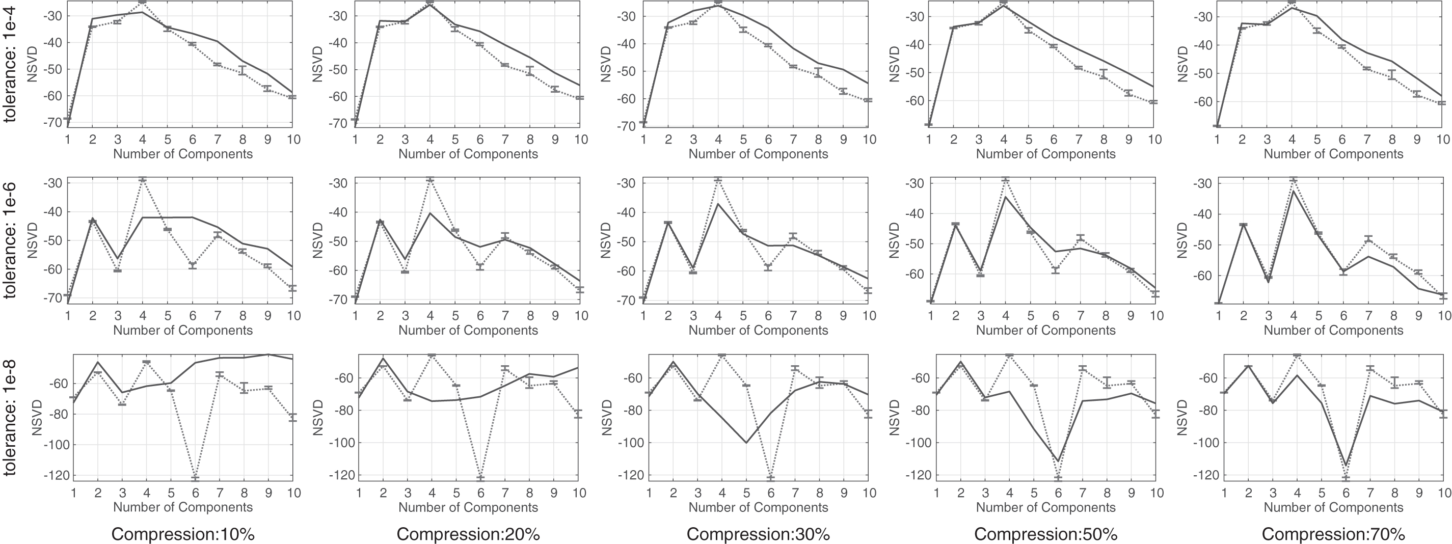
NSVD on the Chem1 data set for tighter tolerances from the top to bottom and lighter compressions from the left to right. At each tolerance level, the dotted lines represent NSVD on Chem1 without compression. For ease of reading, the figure can be viewed online.

In cases where it is not clear what this tolerance level is, an approach could be to perform very tight compressions in the beginning and scan NSVD at various tolerances. If no significant hint of structure is identified, we repeat the procedure for slightly lighter compressions, until a proper indication of a structure appears.

Conclusions

We proposed a new method called NSVD for discovering low-rank multilinear structure in multiaspect data, which are based on the variance of the singular values of the Khatri–Rao product formed by the PARAFAC factor matrices. We have also shown various advantageous theoretical properties of our method, and we argued against a crucial theoretical shortcoming of CORCONDIA. Next, we offered extensive experimental evaluation on both artificial and real data, which verified that our method can be superior compared with other widely used structure finding heuristics. Additionally, we showed an interesting property of our method that allows it to discover different levels of structure in the data. Finally, we suggested the use of an efficient compression scheme and analyzed it both theoretically and experimentally, showing its effectiveness in retaining the original structure in the data.

Footnotes

Acknowledgments

We are grateful to Rasmus Bro for his valuable feedback and for providing us with the chemical data. We are also thankful to Tamara Kolda for bringing to our attention potential shortcomings in our analysis of CORCONDIA.

Disclaimer

Any opinions, findings, and conclusions or recommendations expressed in this material are those of the author(s) and do not necessarily reflect the views of the funding parties.

Author Disclosure Statement

No competing financial interests exist.

Funding Information

This research was supported by the National Science Foundation CDS&E Grant number OAC-1808591 and by the Department of the Navy, Naval Engineering Education Consortium under award number N00174-17-1-0005.

Cite this article as: Tsitsikas Y, Papalexakis EE (2020) NSVD: Normalized Singular Value Deviation reveals number of latent factors in tensor decomposition. Big Data 3:4, xxx–xxx, DOI: 10.1089/big.2020.0074.

Abbreviations Used

Appendix

References

Sun

J-T

, Zeng

H-J

, Liu

, et al. Cubesvd: A novel approach to personalized web search. Proceedings of the 14th international conference on World Wide Web. Chiba, Japan: ACM, 2005. pp. 382–390.

Alex

, Vasilescu

, Terzopoulos

Multilinear analysis of image ensembles: Tensorfaces. European Conference on Computer Vision. Copenhagen, Denmark: Springer, 2002. pp. 447–460.

Howell

TD.

Global properties of tensor rank. Linear Algebra Appl. 1978; 22:9–23.

Kruskal

JB.

Three-way arrays: Rank and uniqueness of trilinear decompositions, with application to arithmetic complexity and statistics. Linear Algebra Its Appl. 1977; 18:95–138.

Carroll

, Chang

J-J

. Analysis of individual differences in multidimensional scaling via an n-way generalization of “eckart-young” decomposition. Psychometrika. 1970; 35:283–319.

Harshman

RA.

Foundations of the Parafac Procedure: Models and Conditions for an “Explanatory” Multimodal Factor Analysis. University Microfilms, Ann Arbor, MI: UCLA Working Papers in Phonetics, 1970, pp. 1–84.

Bläser

A 5/2n 2-lower bound for the multiplicative complexity of n

\times

n-matrix multiplication. Annual Symposium on Theoretical Aspects of Computer Science. Dresden, Germany: Springer, 2001. pp. 99–109.

Bini

DA.

The role of tensor rank in the complexity analysis of bilinear forms. Presentation at ICIAM07, Zürich, Switzerland, 2007.

Derksen

Matrix completion and tensor rank. Linear Multilinear Algebra. 2016; 64:680–685.

10.

Håstad

Tensor rank is np-complete. J Algorithms. 1990; 11:644–654.

11.

Hillar

, Lim

L-H

. Most tensor problems are np-hard. J ACM. 2013; 60:45.

12.

Bro

, Kiers

HAL

. A new efficient method for determining the number of components in parafac models. J Chemom. 2003; 17:274–286.

13.

da Costa

JPCL

, Haardt

, Romer

Robust methods based on the hosvd for estimating the model order in parafac models. In 2008 5th IEEE Sensor Array and Multichannel Signal Processing Workshop. IEEE, 2008, pp. 510–514.

14.

Pouryazdian

, Beheshti

, Krishnan

. Candecomp/parafac model order selection based on reconstruction error in the presence of kronecker structured colored noise. Digit Signal Process. 2016; 48:12–26.

15.

De Silva

, Lim

L-H

. Tensor rank and the ill-posedness of the best low-rank approximation problem. SIAM J Matrix Anal Appl. 2008; 30:1084–1127.

16.

Papalexakis

EE.

Automatic unsupervised tensor mining with quality assessment. In Proceedings of the 2016 SIAM International Conference on Data Mining. SIAM, 2016, pp. 711–719.

17.

Bro

Multi-way analysis in the food industry-models, algorithms, and applications. In Proceedings of ICSLP 2000 MRI, EPG and EMA. Citeseer, 1998.

18.

Lev-Ari

Efficient solution of linear matrix equations with application to multistatic antenna array processing. Commun Inf Syst. 2005; 5:123–130.

19.

Bro

, Andersson

. Improving the speed of multiway algorithms: Part II: Compression. Chemometr Intell Lab Syst. 1998; 42:105–113.

20.

Sidiropoulos

, Papalexakis

, Faloutsos

. A parallel algorithm for big tensor decomposition using randomly compressed cubes (paracomp). 2011 IEEE International Conference on Acoustics, Speech and Signal Processing (ICASSP). Florence, Italy: IEEE, 2014.

21.

Tsitsikas

, Papalexakis

. The core consistency of a compressed tensor. In: Data Science Workshop. Minneapolis, MN: IEEE, 2019.

22.

Bader

, Kolda

. Algorithm 862: MATLAB tensor classes for fast algorithm prototyping. ACM Trans Math Softw. 2006; 32:635–653.

23.

Kolda

, Bader

, Sun

, et al. Matlab tensor toolbox version 2.6, February 2015. Available online at https://gitlab.com/tensors/tensor_toolbox (last accessed July 23, 2020).

24.

Andersson

, Bro

. The n-way toolbox for matlab. Chemometrics and Intelligent Laboratory Systems. 2000; 52:1–4. Available online at https://www.mathworks.com/matlabcentral/fileexchange/1088-the-n-way-toolbox (last accessed July 23, 2020)

25.

Eagle

, Pentland

. Reality mining: Sensing complex social systems. Pers Ubiquit Computing. 2006; 10:255–268.

26.

Eagle

, Pentland

. Eigenbehaviors: Identifying structure in routine. Behav Ecol Sociobiol. 2009; 63:1057–1066.

27.

Eagle

, Pentland

, Lazer

. Inferring friendship network structure by using mobile phone data. Proc Natl Acad Sci. 2009; 106:15274–15278.

28.

Papalexakis

, Akoglu

, Ience

Do more views of a graph help? community detection and clustering in multi-graphs. Proceedings of the 16th International Conference on Information Fusion. Istanbul, Turkey: IEEE, 2013. pp. 899–905.

29.

Diesner

, Frantz

, Carley

. Communication networks from the enron email corpus “it's always about the people. enron is no different.” Comput Math Organ Theory. 2005; 11:201–228.

30.

Klimt

, Yang

The enron corpus: A new dataset for email classification research. European Conference on Machine Learning. Pisa, Italy: Springer, 2004. pp. 217–226.

31.

Bader BW, Harshman RA, Kolda TG. Pattern analysis of directed graphs using dedicom: An application to enron email. Technical Report. Albuquerque, NM: Sandia National Laboratories. 2006.

32.

Pasricha

, Gujral

, Papalexakis

. Identifying and alleviating concept drift in streaming tensor decomposition. Joint European Conference on Machine Learning and Knowledge Discovery in Databases. Dublin, Ireland: Springer, 2018. pp. 327–343.