




Abstract
Context information is the key element to realizing dynamic access control of big data. However, existing context-aware access control (CAAC) methods do not support automatic context awareness and cannot automatically model and reason about context relationships. To solve these problems, this article proposes a weighted GraphSAGE-based context-aware approach for big data access control. First, graph modeling is performed on the access record data set and transforms the access control context-awareness problem into a graph neural network (GNN) node learning problem. Then, a GNN model WGraphSAGE is proposed to achieve automatic context awareness and automatic generation of CAAC rules. Finally, weighted neighbor sampling and weighted aggregation algorithms are designed for the model to realize automatic modeling and reasoning of node relationships and relationship strengths simultaneously in the graph node learning process. The experiment results show that the proposed method has obvious advantages in context awareness and context relationship reasoning compared with similar GNN models. Meanwhile, it obtains better results in dynamic access control decisions than the existing CAAC models.
Introduction
With the rapid development of big data, the demand for manageable and controllable resources is increasingly prominent. Access control is the key technology to ensure the secure sharing of big data resources and prevent unauthorized access. However, compared with the data resources in traditional information systems, big data resources have new characteristics such as large data volume, dynamic generation, multisource heterogeneity, and multiassociation. Users usually request access to resources (information, services, etc.) anytime and anywhere, but the access scenarios also change dynamically. In this dynamically changing environment, users' permissions are related to static elements (e.g., identities, roles, and inherent attributes) and are affected by dynamic elements (e.g., time, place, entity relationships, and access intent or purpose).
Big data systems urgently need to perform authorization and access control according to relevant access scenarios, change user permissions according to the dynamic changes of access scenarios, and control user access dynamically. For example, users are not allowed to access system data resources during nonworking hours and are denied to continue accessing resources when the user is not at the same location range as the data resources. Traditional static policy-based classical access control models, such as discretionary access control (DAC), mandatory access control (MAC), and role-based access control (RBAC), cannot meet the requirements of big data access control. 1
To achieve dynamic access control according to the change of access scenarios, context-aware access control (CAAC) 2 allows flexible and dynamic access control of user access to resources in different “context” information scenarios. 3 Context information 4 is used to describe the state of specific entities related to access control (e.g., users, resources, or environments) and the state of relationships between different entities. For example, information such as user type, resource category, time, location, interentity relationship, and access intent can be considered context information for access control.
In the CAAC model, context awareness5,6 is the premise and basis of dynamic access control using context information, including the steps of obtaining, modeling, and reasoning. However, the existing context-aware methods for dynamic access control have the following two limitations: first, the existing methods do not support automatic context awareness.2,7 When context-based access control rules are formulated, it is necessary to learn the types and fetching values of contexts in advance and determine the change range of the corresponding contexts in the rules to realize dynamic control of subject access. However, the current CAAC model requires the administrator to specify the type of context information in the rule, and the range of its value changes manually. Defining context information manually by experts has a high cost, and the complete context information cannot be defined in advance.
The other limitation is the lack of automatic modeling and reasoning of context relationships.8,9 Many context types are involved in big data systems, and each type may include multiple component elements. Also, there are various associations in these context types according to the access situation. These associations are important for the formulation of context-aware and context-based access control policies. Therefore, when setting context-based access control rules, it is necessary to infer compound and implicit context information and the relationship between contexts from the basic context information, for example, inferring that the subject and object are located in the same place based on the context information. However, the current CAAC model mostly defines ontology to model the context manually, and the administrator makes relevant inference rules. However, the relationship between context information cannot be established automatically, and the established context relationship is fixed and cannot be changed with the context state.
Therefore, it is urgent to develop an automatic and efficient context-aware method to obtain the context scenarios when accessing big data and to model and reason the correlations between context information nonmanually. In this way, intelligent decision-making on big data access control can be achieved.
To solve the above problems, this article integrates the ideas of Stoller and colleagues10,11 and Karimi and Aldairi 12 for mining access control-related elements using logs and the ideas of Fan et al., 13 Xia et al., 14 and Yu et al. 15 for personalized application recommendation using neural networks. Based on this, this article proposes a WGraphSAGE-based context-aware method for big data access control. The method obtains the original context information from user access records and introduces multigraphs 16 and weighted graphs 17 to model the context information. Based on this, the proposed method transforms the access control context-aware problem into an inductive learning and clustering problem of graph node representation. Then, it improves the neighbor sampling and aggregation algorithms in the GraphSAGE model to generate the low-dimensional embedding information of graph nodes.
The vector information output by the algorithm is clustered and calculated to obtain context clusters, thus realizing automatic learning of context information and automatic reasoning about context relationships. Finally, the access control rules are automatically generated from the context scenarios to realize dynamic access control of user access requests based on the context information.
The main contributions of this article are threefold:
A graph neural network (GNN)-based access control context-aware approach is proposed. To the best of our knowledge, GNNs are applied to extract context information for access control for the first time. This article performs graph modeling of the access record data set to transform the access control context-awareness problem into a GNN node learning problem. The method constructs a weighted graph of context information by taking the context information in user access records as graph nodes and the relationships between context as edges. Then, the graph node representation learning is realized by the GNN, and the node embedding information containing node features, node relationship features, and node relationship strength is obtained. Correspondingly, the context information containing context features, context relationships, and their strengths is obtained. A GNN model, WGraphSAGE, is proposed. First, the multivariate vectors of access records are taken as input to obtain the original context information; then, the context information is modeled by graph construction and weighted graph transformation; subsequently, the node embedding of context information is learned by weighted neighbor sampling and weighted aggregation functions; afterward, the context scenario information is inferred by a clustering algorithm; finally, context scenarios are used to automatically generate access control rules to achieve dynamic control on access requests. Weighted neighbor sampling algorithm and weighted aggregation algorithm are designed. The original GraphSAGE
18
model uses equivalent random sampling and aggregation methods, which ignores different effects of neighbor nodes with different weights on node representation. To overcome these shortcomings, this article designs a weighted neighbor sampling algorithm and a weighted aggregation algorithm, which are based on different weight information for neighbor sampling and aggregation calculation. The obtained graph node embedding information contains the feature information of the nodes and their neighbor nodes and incorporates the respective weight information of the related nodes. In this way, these algorithms achieve automatic modeling and reasoning of context relationships.
The rest of the article is organized as follows. In the Related Work section, the work related to GNNs is briefly overviewed. In the WGraphSAGE Model section, a context-aware method based on the WGraphSAGE model is proposed for big data access control. In the Weighted Neighbor Sampling and Weighted Aggregation Algorithms section, the weighted neighbor sampling and weighted aggregation algorithms are designed. The proposed method is experimentally validated in the Experiment Analysis section and finally concluded in the Conclusion section.
Related Work
Dynamic access control
Traditional access control
Traditional access control models, such as DAC, MAC, and RBAC, assign privileges to users that are granted in advance in a static and unchanging manner. Access to big data systems involves different types of dynamically changing contextual information, but these models cannot dynamically change permissions based on the context information at the time of access, nor can they adapt to the constantly dynamic changing context scenarios.
To support dynamic access control decisions, traditional access control models have been extended by adding support for context. For example, the RBAC model adds dynamic elements such as time information, 19 spatial information, 20 and combined time and location information 21 to dynamically activate the roles and their corresponding permissions. However, these improved models can only attach specific types of context information to the original model, only support limited types of context information, and do not consider other types of context information such as entity relationships and access purposes.
The attribute-based access control (ABAC) model provides dynamic access control through global “environmental conditions.” 22 In a broad sense, the environmental conditions of ABAC can also be regarded as context information. However, the environment conditions of ABAC only include part of the public context conditions, such as time and place. These conditions cannot well support the dynamic change of access rights caused by the subject and object's context, such as subject state and subject–object relationship.
Context-aware access control
CAAC enables dynamic control of access behaviors based on different scenarios. Kayes et al. proposed a basic framework for CAAC based on semantic, 4 and then they extended the context conditions in CAAC policies23,24 mainly including basic context information such as users, resources, and their surroundings (e.g., user profiles), user locations, and user request times. Kayes et al. introduced relational context information 25 (e.g., relationship type, relationship strength) into access control policies and proposed a relationship ontology for dynamically identifying entity relationships and relationship strength at different granularities.
Bui et al. mined subject relationships by decision trees in ReBAC, 26 but only the relationship context was considered, and no other contextual information was considered. The purpose of accessing resources or user intent is also an important aspect of context conditions to be considered, and the literature9,27 proposes an ontology-based CAAC approach that incorporates context information such as access purpose and access intent into CAAC policies. The abovementioned studies have extended the context types, but most of them only consider the acquisition and awareness of some types of contexts.
Context awareness is a key aspect of CAAC policy formulation and implementation. Kayes et al. modeled the context through ontology24,28 and semantic ontology languages such as OWL, RDF, and RDF Schema. This method realizes inference and knowledge extraction and provides rich context expressions and validation. However, the ontology and inference rules need to be defined manually by experts. So, the method is not efficient enough and cannot be dynamically updated, and it may cause missing context information, which is not suitable for large data resource access scenarios. To address the problem of CAAC in distributed computing environments such as cloud computing platforms and Internet of Things, Kayes et al. 8 proposed a multisource CAAC model to securely control information resources from multiple data sources based on context.
Kayes et al. 7 presented a CAAC approach based on fog computing with simple management and good scalability in controlling data from multiple sources with a large number of users. However, these methods also define ontologies and formulate context reasoning rules manually, and they cannot automatically model context and reason about relationships, which also reduces the efficiency of context awareness.
Currently, automatic discovery and mining of context information are ignored in the research on access control rule mining. For example, Stoller and colleagues mined authorization rules from access control logs and attributes 10 but did not model and reason about “environmental conditions.” Karimi and Aldairi performed clustering operations on preprocessed logs. 12 Although the environmental conditions in the rules were considered, the relationships between environmental conditions were not considered. Das proposed a policy mining method based on the Gini coefficient to mine the policies that support environmental attributes. 29 Meanwhile, the method of building decision trees was used for policy construction. However, the method fails to fully explore the relationships between environmental conditions and access scenarios.
The above research on CAAC dynamically controls access to information resources through a CAAC model, where the context-type information is extended and context-aware methods are designed. However, these methods cannot support automatic awareness of context types and fetch ranges and fail to perform automatic modeling and reasoning about context relationships, 2 which will affect the learning results and execution efficiency of CAAC rules.
Graph neural networks
Development of GNN
Deep learning has become an important approach to achieving artificial intelligence. Traditional deep learning models, such as convolutional neural networks (CNN) and recurrent neural networks, are suitable for processing the data in Euclidean space, such as images (two-dimensional network data) and text (one-dimensional sequence data). However, graph-structured data such as access records, entity relationships, and molecular structures do not have the characteristics of translation invariance in Euclidean space. Therefore, traditional neural network models cannot be directly applied to the learning and inference of graph data.
The concept of GNNs 30 was first proposed in 2005, and GNNs can capture graph dependencies through the message passing of nodes in a graph. 31 In recent years, many variants of GNNs, such as graph convolutional network (GCN), 32 graph attention network, 33 and GraphSAGE, 18 have achieved breakthroughs in many deep learning tasks. With these models, the purpose of mapping each node in the graph to a low-dimensional vector can be achieved. This vector representation is often called node embedding,34,35 which preserves the key information of the nodes in the original graph.
Graph convolutional network
The concept of GNNs was defined by Scarselli et al. in 2009 in his article. 31 GCN 32 was the first to apply the convolution operations in image processing to graph-structured data processing. GCN is a multilayer graph CNN, where each convolutional layer processes only first-order neighborhood information. Meanwhile, by superimposing several convolutional layers, information transfer in multiorder neighborhoods can be achieved. The advantage of GCN is that it can capture the global information of a graph and represent the features of the node well.
GCN can be used for various downstream applications such as classification of prediction graph nodes, prediction of edges, and subgraph prediction. Yu et al. 15 proposed a GCN-based representation learning model called Semantic-Aware-GCN, which maps applications, locations, and time units into dense embedding vectors for application prediction. However, since this method is based on the GCN model, it is also limited by transductive node representation. Also, the method requires prior learning of all nodes of the whole graph, and so, it does not support the expansion of multiple types of context information due to its spatiotemporal characteristics and unit properties.
GraphSAGE
To overcome the shortcomings of GCN, Hamilton et al. proposed the GraphSAGE model based on an inductive framework. 18 It transforms “learning the representation of each node” into “method for learning the representation of each node” by randomly sampling the information of a node from its neighbors and then using a selected aggregation function to obtain the feature representation of the node. The output feature representation incorporates the feature information of a node and its neighboring nodes, reflecting the relationship between nodes.
The limitations of GraphSAGE are as follows: (1) it cannot handle weighted graphs, and can only perform equal-weight aggregation of neighboring nodes; and (2) random equal-length sampling can lead to the loss of important local information of some nodes, and the features of the same node embedding in the inference stage are unstable.
User access records are multivariate, multidimensional data, and there are correlations between the records. Thus, user access records can be modeled with a graph structure, and the feature information in this graph can be learned by the GraphSAGE model. However, the model does not consider the different weight coefficients of neighboring nodes and cannot handle heterogeneous nodes. Therefore, when the model is applied to learn user access records, the problems of weight calculation and normalization of heterogeneous nodes need to be solved.
PinSage 36 improves on GraphSAGE. It eliminates the limitation of storing the entire graph in GPU memory and uses low-latency random wandering to sample graph neighborhoods in a producer–consumer architecture. However, it cannot distinguish between different classes of features of individual nodes and cannot support interaction between composite nodes. The core problem studied by the PinnerSage model 37 is how to use the item embedding already learned by PinSage to generate user embedding and complete user2item recall. However, it does not use GNNs and likewise cannot support the interaction between composite nodes.
MultiSage 38 proposed a contextual GCN engine to model multidimensional GNNs for the target nodes and their contextual nodes. Contextual nodes in the MultiSage model are related nodes in different scenarios relative to the target node and belong to different classes of nodes from the target node. For example, Pin in Pinterest is the target node, while Board is the context node, and the categories of the two are not the same. Therefore, the context nodes of MultiSage are different from the access control contexts mentioned in this article. In addition, MultiSage does not support the combination of multiple category context features and cannot meet the need of combining multiple context features present in the access logs for learning.
WGraphSAGE Model
To realize the acquisition and inference of context scenario information from user access records, this article proposes a new weighted GNN model called WGraphSAGE based on GraphSAGE. In WGraphSAGE, the set of user access records is transformed into a graph structure, and weighted neighbor sampling and weighted aggregation algorithms are designed to learn the weighted representation of graph nodes. Then, the learned node embedding information is clustered to generate context scenario information. The context scenario can be used to automatically generate access control rules, thus enabling dynamic control of user access based on context information. The proposed model overcomes the problem that the original GraphSAGE model cannot distinguish the importance of neighbor nodes and does not support multiple types of node features due to the “equal-weight” calculation.
Compared with the existing CAAC model, WGraphSAGE achieves automatic awareness of context type and range of values, and it can perform automatic modeling and reasoning of context relationships.
Problem and related definitions
Context information 4 is used to describe the status of access control-related entities such as users, resources, or environments, the relationships between different entities, access purpose, and so on. According to the definition of context in the literature and considering the requirements of dynamic access control of big data, the definitions of context scenario and context awareness in access control applications are given, and they are used as the basis for problem formulation.
The goal of this article is to perceive context scenarios from user access records through WGraphSAGE, which is formulated as follows:
where D is the access record set; CS is the context scenario set, and WG denotes the WGraphSAGE model.
The learning goal of the WGraphSAGE model is to obtain high-quality context scenarios, that is, context scenarios that preserve the features of the context information in the access records and the relationships between the context information.
In this article, multigraphs are used to model context information features and relationships, and multigraphs are defined as
where distance j is the Minkowski distance of the feature vector of the jth element. The threshold for DoE (TfD) 34 indicates the threshold for determining the existence of an edge based on the corresponding element distance. TfD j denotes the distance threshold of the jth element.
If the DoE does not exceed the threshold, then the two nodes in the graph correspond to similar elements and an edge exists between them,

Model framework
In this article, the context-awareness problem is transformed into a graph representation learning problem, and “edge weights” is introduced into the GNN to accurately represent context information features and relationships. Based on this, a weighted GraphSAGE model is proposed for context awareness, and the model framework is shown in Figure 1.
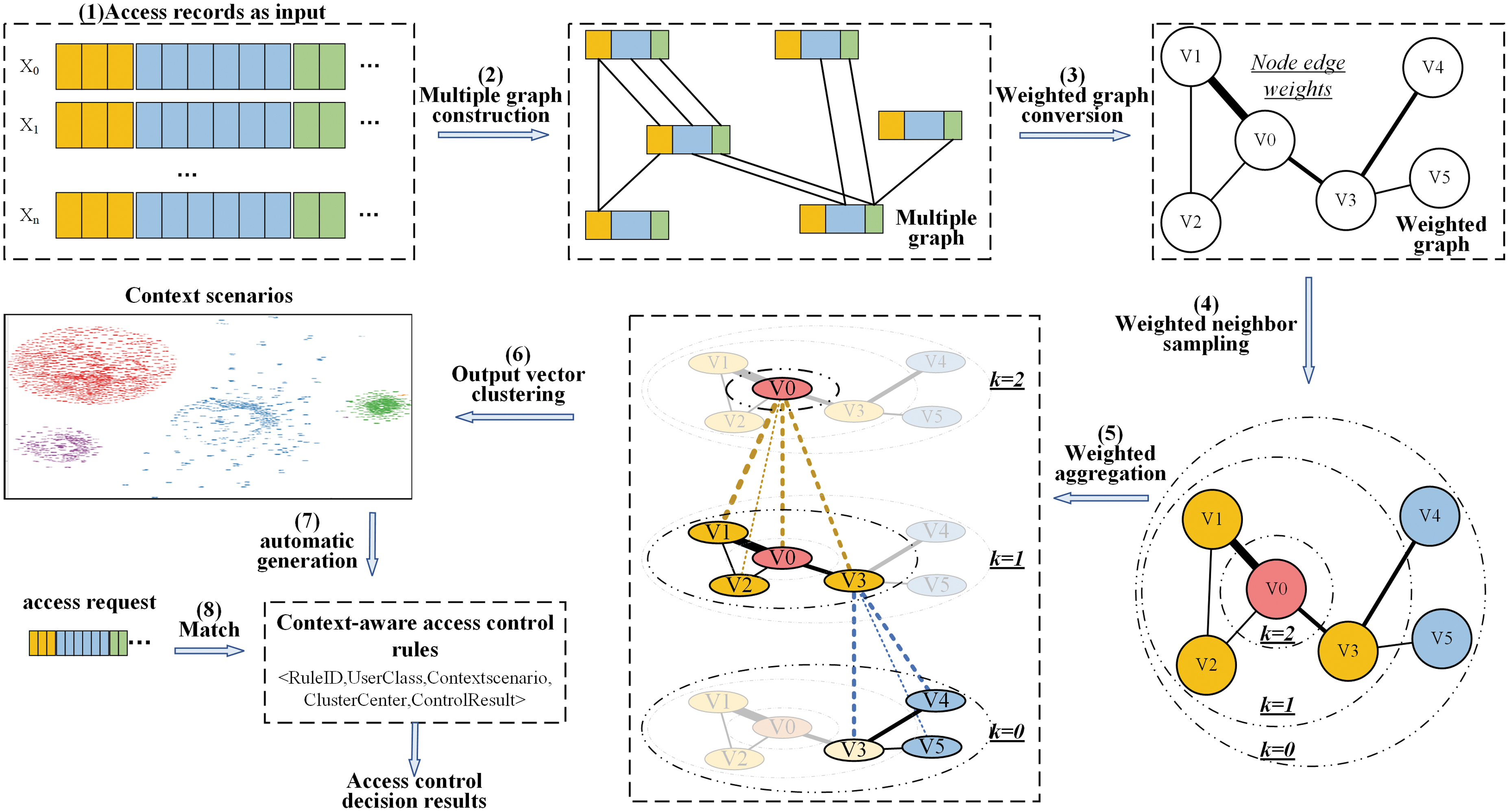
The framework of the WGraphSAGE model. WGraphSAGE, Weight Graph Sample, and aggreGatE.
Step 1: a set of user-access records containing multivariate vectors are used as the input to the model. Each access record includes multiple types of information such as subject (user), object (resource), access operation (read, write, add, delete, update, etc.), context (time, location, subject–object relationship, etc.), and each type of information contains one or several pieces of vector information.
Step 2: multigraph construction. Each access record is treated as a node of the graph, and the input features of the node consist of multiple elements. Each input feature has the same kind and number of elements, but the elements may have the same or different values. When the vector value of the corresponding element distance (DoE, Definition 4) does not exceed the element distance threshold, an element edge (EfE, Definition 5) is added between the corresponding elements of the two nodes, and the number of element edges between the two nodes is 0 to m (m is the number of elements).
Step 3: weighted graph conversion. To facilitate GNN learning without losing the relationship between edges of nodes, the graph is converted to a weighted graph by normalization methods. The weighted graph has no or one edge between nodes, and the weight of an edge (WoEfN, Definition 9) is the sum of the corresponding element weights (WoE, Definition 8).
Step 4: weighted neighbor sampling. Following the minibatch idea of GraphSAGE, the neighbors of nodes in the graph are sampled layer by layer according to the inside-out method. To distinguish different association relationships between nodes, this article adds the variable of node edge weight W′ to the sampling function, and the neighboring nodes having edges with higher weights are sampled preferentially.
Step 5: weighted aggregation. Based on the weighted sampling, the nodes in the graph are aggregated one by one, from the outer layer to the inner layer, to generate the embedding information of the nodes.
Step 6: the output node embedding information is clustered to obtain a set of context scenario information. Each element in the set corresponds to a context scenario.
Step 7: the context scenarios obtained by clustering are automatically generated into corresponding access control rules.
Finally, when an access request is received, it is transformed into a feature vector containing context information. The feature vector of the access request is matched with the access control rules to obtain the final decision result.
Multielement data preprocessing
User access records are taken as the original input data, and each data record includes multiple types of information such as subject, object, access operation, and context. Each type of information contains one or more vectors of information.
Assume that the set of access records D contains n + 1 unlabeled samples (i.e., access records), D = {X0,X1,…,Xi,…,Xn},
Multigraph construction
The set of user access records is a multielement, multidimensional, multifeatured data set, and there may be multiple relationships among the context information in the records. This article represents the data set by constructing a multigraph to learn the context features, potential patterns, and internal relationships of user access.
In this article, a multigraph
If the corresponding multiple pairs of elements in two access records take similar or identical values, there are multiple relationships between these two access records. For instance, there will be two relationships (same time, same place), if the access times and the access locations are the same. These relationships can be represented by creating multiple edges between the corresponding nodes of these two access records.
Suppose that the graph node Vi contains m elements (Definition 3). Then, the set of user access records corresponds to the set of nodes of the graph
When the DoE (Definition 4) of the corresponding elements of two nodes is less than TfD, it indicates that the two nodes are related, that is, the two access records contain the same or similar context elements, and an undirected EfE (Definition 5) is established for the corresponding elements of the two nodes. If there are multiple pairs of elements that are identical or similar, multiple EfE are established, which indicates that there are multiple context information elements that are identical or similar for the two access records. The higher the number of the EfE between two nodes, the closer the relationship between the two nodes. To count the number of elemental edges, the sign of EfE (s, Definition 6) is used to indicate whether the two nodes have EfE for the corresponding elements. Multiple signs of EfE are formed into the SV (Definition 7).
Weighted graph conversion
Based on the relationship of corresponding elements in nodes, the multigraph describes the multiple relationships between nodes. However, the existence of multiple element edges between two nodes does not facilitate the learning of GNN models. To this end, this article introduces the weights of edges to transform multiple edges into weighted edges and accordingly transforms the multigraph into a weighted graph. A weighted graph is a graph model that associates a weight or cost to each edge, that is, a weight is added to each edge on top of a simple graph.
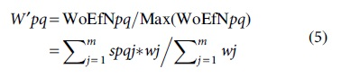
The process of transforming a multigraph into a weighted graph is shown in Figure 2. If there is one EfE or multiple EfE between two nodes Vp and Vq, the EfE can be changed to one edge for nodes uniformly, and the WoEfN (Definition 9) can be calculated by using SV with the WoE (Definition 8) as follows.

Conversion of multigraphs to weighted graphs.
To facilitate the subsequent data processing and calculation, the values of WoEfN are obtained by minimum–maximum normalization.
when
Weighted neighbor sampling and weighted aggregation
The random neighbor sampling and aggregation functions are key aspects of the original GraphSAGE model. However, the neighbors of nodes in this model are “equal” and have the same relationship with each other. If random neighbor sampling and aggregation functions are adopted, the relationship between nodes cannot be reflected with different weights. Therefore, this article proposes weighted neighbor sampling and weighted aggregation algorithms for the GraphSAGE model, and the details and analysis of the algorithms are described in the Weighted Neighbor Sampling and Weighted Aggregation Algorithms section. After learning with this algorithm, the output node embedding information includes the key features of nodes, node relationships, and the closeness of the relationships, which supports the subsequent context scenario learning.
Weighted neighbor sampling
In the sampling algorithm of the GraphSAGE model, a fixed number of neighbors are randomly sampled for each node, and the neighbors are undifferentiated. In the weighted graph constructed in this article, due to the existence of weights on the edges between nodes, the importance of node neighbors and its influence on the representation of nodes are different. Therefore, the neighbor nodes are sampled with a different probability, that is, the nodes with high edge weights are sampled with a high probability, and those with low edge weights are sampled with a low probability. According to the idea of the weighted random sampling algorithm, 39 the probability of selecting a neighbor node is calculated as the ratio of the edge weight of the node to the sum of the edge weights of all neighbor nodes.
Weighted aggregation
In the aggregation algorithm of the GraphSAGE model, each neighbor is equivalent when the aggregation operation is performed on the node's neighbor feature information. As for the weighted graph constructed in this article, since the edge weights of the nodes and different neighboring nodes are not identical, then the contribution of a node's neighbors to aggregation is not exactly the same, and the influence of edge weights on the aggregation function should be considered. Therefore, in this article, the factor of node edge weights is added to the weighted aggregation algorithm.
In addition, the graph includes a large number of nodes and edges. If the whole graph is loaded, a huge number of samples need to be processed for each iteration, which decreases the training efficiency of the GCN. To improve the learning efficiency and gradient descent speed of the graph, this article trains the graph in multiple small batches.
Clustering of node embedding
After learning by the WGraphSAGE model, the node embedding information is output, which retains the feature information of the input data in the low-dimensional vector data and incorporates the association information between the nodes in the graph structure. Two types of association are involved: multiple relationships and multiple weights (different closeness degrees of the relationship). The feature vector of node embedding information can be used for downstream computations and applications. Meanwhile, the node clusters (sets) that cluster the access records with the same or similar context information can be obtained by a clustering operation on the feature vector. Then, the feature description of this node cluster can be used to describe the corresponding context scenario information.
In this article, the feature vectors of node embedding information are clustered by the K-means++ algorithm, and the clustering results are presented visually by the t-SNE algorithm. 40 By clustering the node embedding information, the nodes in the same cluster are more closely aggregated, and the nodes in different clusters are less closely aggregated. The clustered results can be used as context scenario information for inference and CAAC policy formulation.
Automatic generation and matching of access control rules
After the node embedding information clustering, each node cluster corresponds to a context scenario, and the feature information of the node cluster represents the feature information of the corresponding context scenario. In this case, the system will automatically formulate CAAC rules based on the clustering results (i.e., context clusters). The CAAC rules are represented as <RuleID, UserClass, Contextscenario, ClusterCenter, ControlResult>, where RuleID denotes the number of the rule, which is the same as the scenario serial number; UserClass denotes the classification identifier of the user, which can be represented by the user role and feature attributes; contextscenario describes the clustering result corresponding to the contextual information; ClusterCenter denotes the feature vector of the clustering center; and ControlResult denotes the access control result.
When an access request is received from a user, the system matches the user request with the CAAC rules that have been automatically generated, queries whether the permission requirements are satisfied, and makes an access control decision. First, the system performs context vector transformation on the received request information to obtain the context information containing m elements. Then, the distance between the request context information and each cluster center is calculated separately. Next, the calculated multiple distance values are ranked, and the cluster center with the closest distance is selected as the matching item. Finally, the access request is responded to according to the access control rules corresponding to the matching term.
Weighted Neighbor Sampling and Weighted Aggregation Algorithms
The main difference between the weighted neighbor sampling and weighted aggregation algorithms and the existing GraphSAGE algorithm is that node edge weights are added to the process of neighbor sampling and aggregation. The node edge weights are multiplied with the corresponding WoEfN and then aggregated. The weighted neighbor sampling and aggregation operations can characterize the weight between nodes and neighbor nodes and distinguish the contribution of the neighbor nodes with different weights to node embedding. The final output node vector representation aggregates more information from “large-weight” neighbor nodes, which helps cluster the context information of closely related neighbor nodes together.
Algorithm design
Weighted neighbor sampling
Unlike random neighbor sampling, the weighted neighbor sampling algorithm first specifies the initial set of nodes. Then, it obtains all first-order neighbor nodes N(u) of the initial set of nodes and the node edges between the nodes and first-order neighbor nodes. Next, it ranks the first-order neighbor nodes by node edge weights and samples Sk nodes from N(u) neighbor nodes according to the reservoir sampling algorithm. 39 Subsequently, the Sk nodes are weighted to sample their respective Sk − 1 neighbor nodes following the above method, and the set of all eligible weighted neighbor nodes is obtained by weighted neighbor sampling layer by layer. k denotes the number of layers to be sampled, and it is usually set to 2 to prevent the problem of oversmoothing. 18
The weighted neighbor sampling process is shown in Figure 3A. In the example, K = 2, S1 = 3, S0 = 2. First, for node V0, in layer 1 (inner layer), three nodes with higher “node edge weight” {V1,V3,V5} are weighted and sampled from all the neighboring nodes {V1,V2,V3,V4,V5}. In layer 0 (outer layer), the first-order neighbor nodes are weighted and sampled separately to obtain two neighbor nodes, resulting in six neighbor nodes {V6,V7,V9,V10,V12,V13}.

An example of weighted neighbor sampling and weighted aggregation.
Weighted aggregation
Different from the aggregation function in GraphSAGE, the weighted aggregation function in this article not only aggregates the representation information of neighbor nodes but also adds the edge weight information between nodes and neighbor nodes.
The weighted aggregation is based on the results of weighted neighbor sampling, and the operation is performed sequentially from the outer layer to the inner layer. First, the outermost neighbor node representation information of each node is multiplied by the node edge weights. Then, these products are aggregated, and the neighbor node aggregation values are connected with the current representation information of the next outer node. Afterward, this connection vector is transformed by the fully connected layer of the nonlinear activation function to obtain the next outer node representation information. By using the representation information of the next outer node, the weighted aggregation operation is continued until it reaches the innermost node.
For example, Figure 3B shows that the weighted sampled neighbors of V0 are {V1,V3,V5}, and the weighted sampled neighbors of V1, V3, and V5 are {V6,V7}, {V9,V10}, and {V12,V13}, respectively. When weighted aggregation is performed for node V1, the neighbor weighted aggregation information of V1 is first calculated as
Where, v1, v3, and v5 denote the feature vectors of nodes V1, V3, and V5, respectively, while w0,1, w0,3, and w0,5 denote the weights of nodes V1, V3, and V5, with respect to node V0, respectively. AGG denotes the name of the aggregation function, and the optional aggregation functions include mean, long short-term memory (LSTM), mean-pooling, and maximum pooling. After aggregation, the representation information of the node is calculated by normalization.
Algorithm implementation
Weighted neighbor sampling algorithm
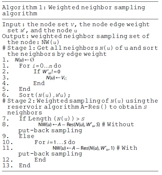
The neighbor sampling function in GraphSAGE adopts a fixed-length random sampling approach. By contrast, the neighbor sampling function NW(u) in this article considers the node edge weight information when sampling the neighbors. The weighted neighbor sampling algorithm is shown in Algorithm 1.
The algorithm is divided into two stages. In stage 1, all first-order neighbor nodes of node u (i.e., the nodes with node edges to u) are obtained from the graph and sorted by node edge weights. The computational complexity of the stage is O(n). In stage 2, S neighbors are obtained by the weighted sampling of N(u) neighbor nodes of u, where S is a predetermined hyperparameter. The work conducted in stage 2 is essentially a weighted random sampling problem with probability weighting, that is, each sample in the sample set has a weight wi > 0 attached to it, and the probability of each sample being sampled is determined by wi.
In this article, reservoir sampling 39 is used to implement the sampling operation. If the number of neighbors N(u) is greater than or equal to the number of sampling targets S, A-Res[N(u), W′u, S] is called without putting back the sampling, where the weight of the sample is W′ u and the reservoir size is S; otherwise, S reservoirs with a size of 1 are created, and for each sample Vi, the A-Res algorithm is run on each reservoir independently with put-back sampling. The computational complexity of stage 2 is O(m*log(n)).
Minibatch weighted aggregation algorithm
Referring to the idea of the minibatch algorithm in GraphSAGE, the minibatch weighted aggregation algorithm is designed in this article. The algorithm process is shown in Algorithm 2.
The symbols of the algorithm are explained as follows. Xv represents the input feature of a node v;

Stage 1: A small batch subset B of node set V is selected as the initial node set BK. Lines 2–7 execute two nested loops of the program body. The first loop performs layer-by-layer weighted sampling from the inside to the outside, and the second loop performs weighted sampling of the neighbors of the nodes in that layer. Starting from the innermost layer BK, the weighted neighbor sampling function NW(u) is called to sample the neighbors of all nodes u in BK, and the sampling results are merged with BK to obtain BK − 1. This process is repeated, and the small-batch weighted sampling set B0 is obtained finally.
Stage 2: Line 8 of the algorithm first initializes the feature vectors of all nodes in the input graph. Lines 9–15 perform two nested loops. The first loop is a layer-by-layer weighted aggregation process from the outside to the inside, and the second loop is a weighted aggregation process for each node u in that layer. In the second loop, line 11 performs weighted aggregation of the neighbor node information of u using the aggregation function, that is, first multiplying the feature information of the neighbor node with the node edge weight (the weight of the edge between node u and its neighbor node) and then aggregating the product.
Line 12 connects the neighbor aggregation information and the current embedding information of node u, and then updates the embedding information of u by nonlinear transformation. Line 13 normalizes the node embedding information. Line 16 takes the final result after two levels of cyclic computation as the output zu, that is, the final node embedding information.
It is important to note that the node edge weights W′ is different from the weight matrix W. This is because W′ is determined when building the weighted graph, while W is the parameter to be learned by the GNN.
Loss function and parameter learning
In this article, context scenario information is modeled and reasoned from the access log data set, which is unlabeled sample data. Thus, the learning of context scenarios belongs to unsupervised learning. The graph-based loss function expects neighboring nodes to have similar vector representations, while nonadjacent, distant nodes are represented as differently as possible. This article uses the loss function of the unsupervised learning method of GraphSAGE, and the function is shown below.
where zu is the output vector of node u (i.e., node embedding); v is the neighboring nodes near u selected by the weighted sampling algorithm; Pn(v) is the probability distribution of negative sampling;
According to the loss function value, the parameter weight matrix Wk and the parameters of the aggregation function are adjusted by the stochastic gradient descent method. 18 As the value of the loss function decreases, the node embedding information better includes the node feature information, the relationship between nodes and neighbors, and the tightness of the relationship.
Experiment Analysis
Experiment settings
Data collection
To validate the proposed WGraphSAGE model and the usability of the algorithm, four data sets of user access records to resources are selected for experimental analysis, including Appusage, 41 Carat, 42 Frappe, 43 and WS-Dream. 44 Each access record includes metadata such as time stamp, location identification, access app identification, and network communication latency, which provides the basic elements for context information awareness.
Input data preprocessing
Step 1: Each access record in the data set is treated as a node, and the corresponding field of each access record is selected as the input data of each node. The data include node number and node element: the node number is a running number ID, and the node element is a <u,t,l,r> quadruplet, including the Userclass, Time, Location, and Resourceclass.
Step 2: Each element of a graph node is represented by a vector, and the vector length of the element is set to L bits so that the total length of the node vector is 4L bits.
Step 3: Create the EfE. If the values of the corresponding elements of two nodes are the same (e.g., Userclass, Location, or Resource is the same), an element edge is created between the corresponding elements of the two nodes. Meanwhile, if the Time element of the two nodes is similar, an element edge is created between the Time elements of the two nodes. All nodes are scanned in turn to establish the element edges between the corresponding elements of all nodes.
Step 4: Establish the EfN and calculate the WoE. In the experiment, the WoE is assumed to be the same, and it is set to 1/4 = 0.25. Based on this, the edge weights between any two nodes are calculated to obtain the weighted graph.
Experiment steps and baseline methods
Since the current CAAC model does not support automatic context awareness, the experiments in this article are divided into three steps: automatic context awareness, CAAC, and ablation experiments.
Step 1: automatic context awareness. In this article, the proposed WGraphSAGE model is compared with the graph representation models Node2vec, 45 GCN, and GraphSAGE, and the results of the proposed model are compared with those of different aggregation functions. After GNN learning, the clustering results and effects of graph nodes are analyzed to compare the running time, clustering evaluation metrics, and so on.
Step 2: CAAC. The access control effect of the WGraphSAGE model is compared with that of OntCAAC 28 and FB-CAAC 7 models.
Step 3: ablation experiments. The impact of weighted neighbor sampling and weighted aggregation algorithms in the WGraphSAGE model on the clustering results of context information and on the effect of access control is analyzed.
Implementation details and parameter settings
Node2vec, GCN, GraphSAGE, and WGraphSAGE models are implemented via TensorFlow. These models are run on a computer equipped with Intel Core i9-10980XE 3.00 GHz CPU and 256 GB DDR4-3200 SDRAM memory. According to the aggregation function selection method, the WGraphSAGE model is subdivided into four cases: mean, seq, maxpool, and meanpool. The parameters of the models are set as follows: the minibatch size is 512; the number of layers of graph aggregation 18 K = 2; the number of samples in each layer S1 = 25, S2 = 10; the output vector Out_dim1 = 128, Out_dim2 = 128, Out_dim = = 256, and the number of negative samples Sneg = 20.
Two models, OntCAAC 28 and FB-CAAC, 7 are implemented through the Java language. To achieve a fair comparison, the model parameters are set with reference to the values in their original articles. The statistical count of the average response time for access control decisions is 10.
Analysis of experimental results
Automatic context-awareness experiments
Running time
Different numbers of graph nodes were selected to run the Node2vec, GCN, GraphSAGE, and WGraphSAGE models. The relationship between the number of nodes and the running time was analyzed, and the result is shown in Figure 4. Figure 4A–C presents the execution time comparison (excluding the time to build the graph) of Node2vec, GCN, GraphSAGE (using the mean function), and WGraphSAGE (using the weighted mean function) on the Appusage, Carat, and Frappe data sets, respectively. Figure 4D presents the comparison of the running time of GraphSAGE and WGraphSAGE using the four aggregation functions on the WS-Dream data set, respectively.
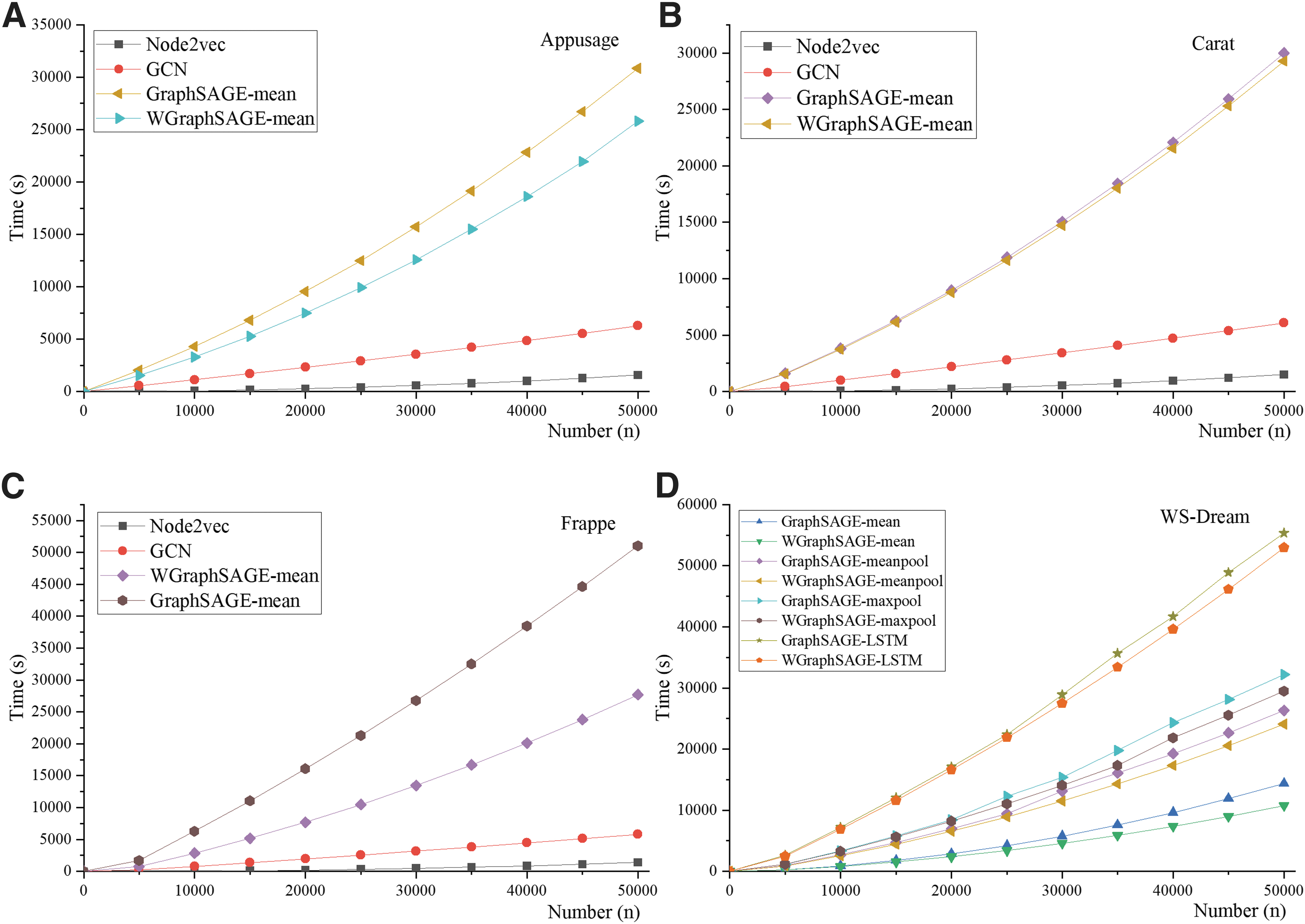
Node quantity–time relationship.
It can be seen from Figure 4A–C that the operation time of the four models increases polynomial with the number of nodes. With the same number of nodes, GraphSAGE and WGraphSAGE consume more operation time than Node2vec and GCN. This is because the aggregation function used in GraphSAGE and WGraphSAGE has a larger overhead than the skip-gram method of Node2vec and the frequency domain graph convolution method of GCN without predicting the unknown node embedding information.
Figure 4D shows that WGraphSAGE has a slightly lower operation time than GraphSAGE when they use the same aggregation function. Specifically, GraphSAGE-mean has a lower operation time than GraphSAGE-mean, and WGraphSAGE-maxpool has a lower operation time than GraphSAGE-maxpool. This is because the GraphSAGE model requires random sampling for each iteration of computation, while the WGraphSAGE model does not require repeated sampling. Although the aggregation function of the GraphSAGE model needs to multiply edge weights with aggregation vectors, the calculation has a constant order of complexity, which does not increase the overhead.
The arrangement of the four aggregation functions in increasing order of operation time is mean<meanpool<maxpool<LSTM. The operation time is only related to the time complexity of the four aggregation functions.
Loss function value
The loss function
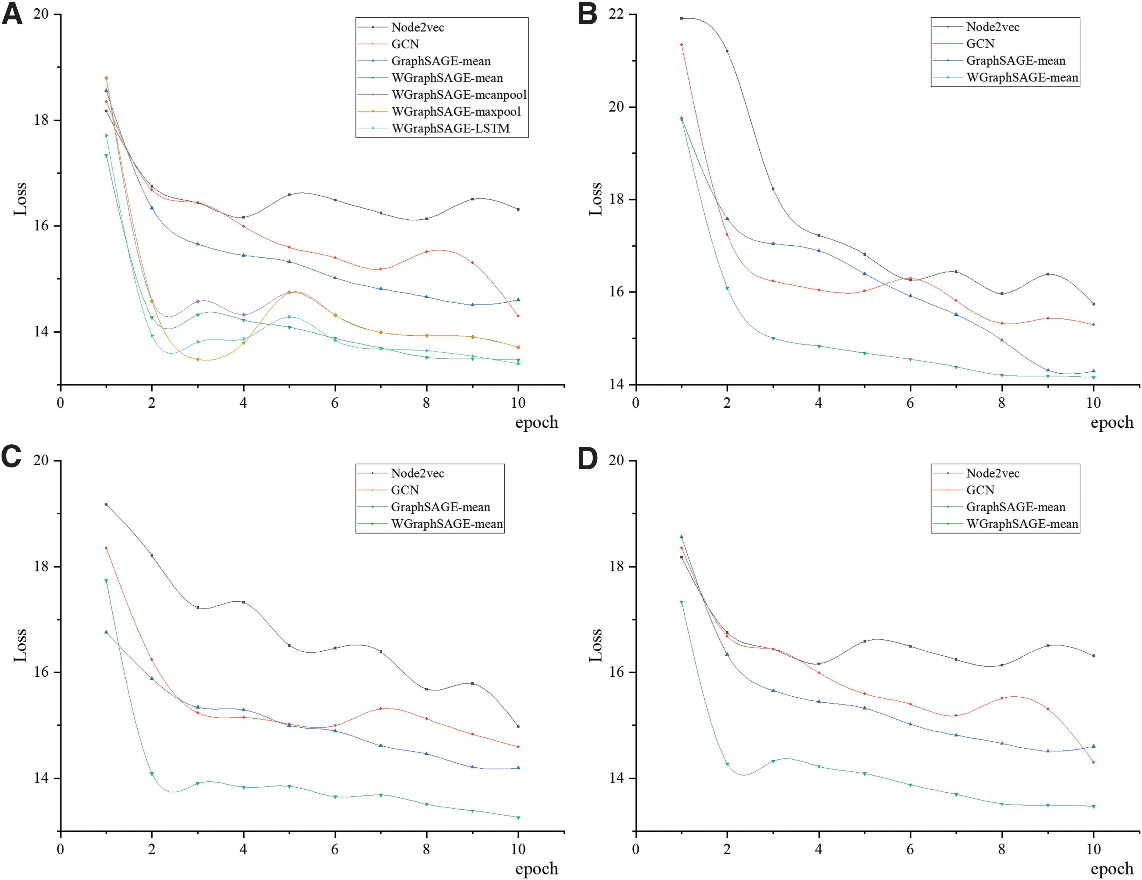
The relationship between the number of iterations and the loss function value.
Figure 5A–D presents the change in loss function values of Node2vec, GCN, GraphSAGE, and WGraphSAGE after several iterations of computation (learning rate is set to μ = 0.0001). The variation of loss function values after iterative computation of WGraphSAGE using four different weighted aggregation functions is also presented in Figure 5A. For each model, the loss function value Loss changes as the number of iterations increases. The proposed WGraphSAGE model has a lower Loss value than Node2vec, GCN, and GraphSAGE.
The loss function value Loss of WGraphSAGE significantly decreases after two iterations; then, with the increase of epochs, the Loss value tends to be stable. This is because after the node edge weight parameter is increased, and the similarity of neighboring nodes and the difference between non-neighboring nodes of WGraphSAGE increases in the process of sampling and aggregation calculation of neighbors.
In addition, WGraphSAGE uses samples of local neighbor nodes and aggregates them by the weight value. After several iterations for all nodes, the parameters of the node embedding method will become relatively stable. In this case, the corresponding Loss value will also be stable during subsequent iterations.
Clustering evaluation metrics
The use of the K-means++ algorithm to perform clustering operations on graph node output vectors requires prior determination of the number of clusters, that is, k_clusters. A popular method for determining the number of clusters in unsupervised learning models is the Elbow method. 46 This method is based on the total sum of the squares within the group, and the current k_clusters will be chosen as the cluster number if adding another cluster does not lead to better modeling of the data (i.e., Elbow point of the graph). However, this method cannot choose the right point when bending occurs.
To overcome the limitation of the Elbow method, the average silhouette (SIL),47,48 Calinski–Harabasz Index (CHI)49,50 and Davies–Bouldin Index (DBI)51,52 methods are adopted in this article to determine the number of clusters, abbreviated as k_clusters.
The process of determining the number of clusters is as follows. First, the clustering algorithm is run with different k_clusters, and SIL, CHI, and DBI values are calculated, respectively. Then, the appropriate k_clusters values are selected when an appropriate combination of SIL, CHI, and DBI values is obtained.
The relationship between k_clusters and SIL, CHI, and DBI values is illustrated in Figure 6A–D, representing the four data sets of Appusage, Carat, Frappe, and WS-Dream, respectively. In Figure 6A, when k_clusters = 203, CHI and DBI reach the optimal value of 21506.02 and 0.36, respectively. At this time, SIL = 0.95, which is the maximum value. The slope of its tangent line decreases significantly, and the value of SIL shows a decreasing trend with the increase of k_clusters. In Figure 6C, when k_clusters = 55, SIL, CHI, and DBI obtain a better value. This is because when k_clusters take the appropriate value, the nodes in the same cluster are more concentrated and those in different clusters are more dispersed.

Cluster number–evaluation index relationship diagram. The relationship between k_clusters and SIL, CHI, and DBI values is illustrated in
Meanwhile, when SIL, CHI, and DBI reach the optimal or better values, it indicates that the clustering of context information reaches the optimal or better state. Therefore, combining these indicators can evaluate the effect of clustering more accurately.
Clustering results
The clustered results are presented by t-SNE dimensionality reduction, as shown in Figure 7. Figure 7A–D represents the clustering results of the subsets of Appusage, Carat, Frappe, and WS-Dream data sets, respectively, while the four columns in the figure represent the clustering results of Node2vec, GCN, GraphSAGE, and WGraphSAGE, respectively. Since the whole access record data set corresponds to a large number of clusters, the number of clusters is briefly indicated here, and 5000 records are randomly selected for analysis.
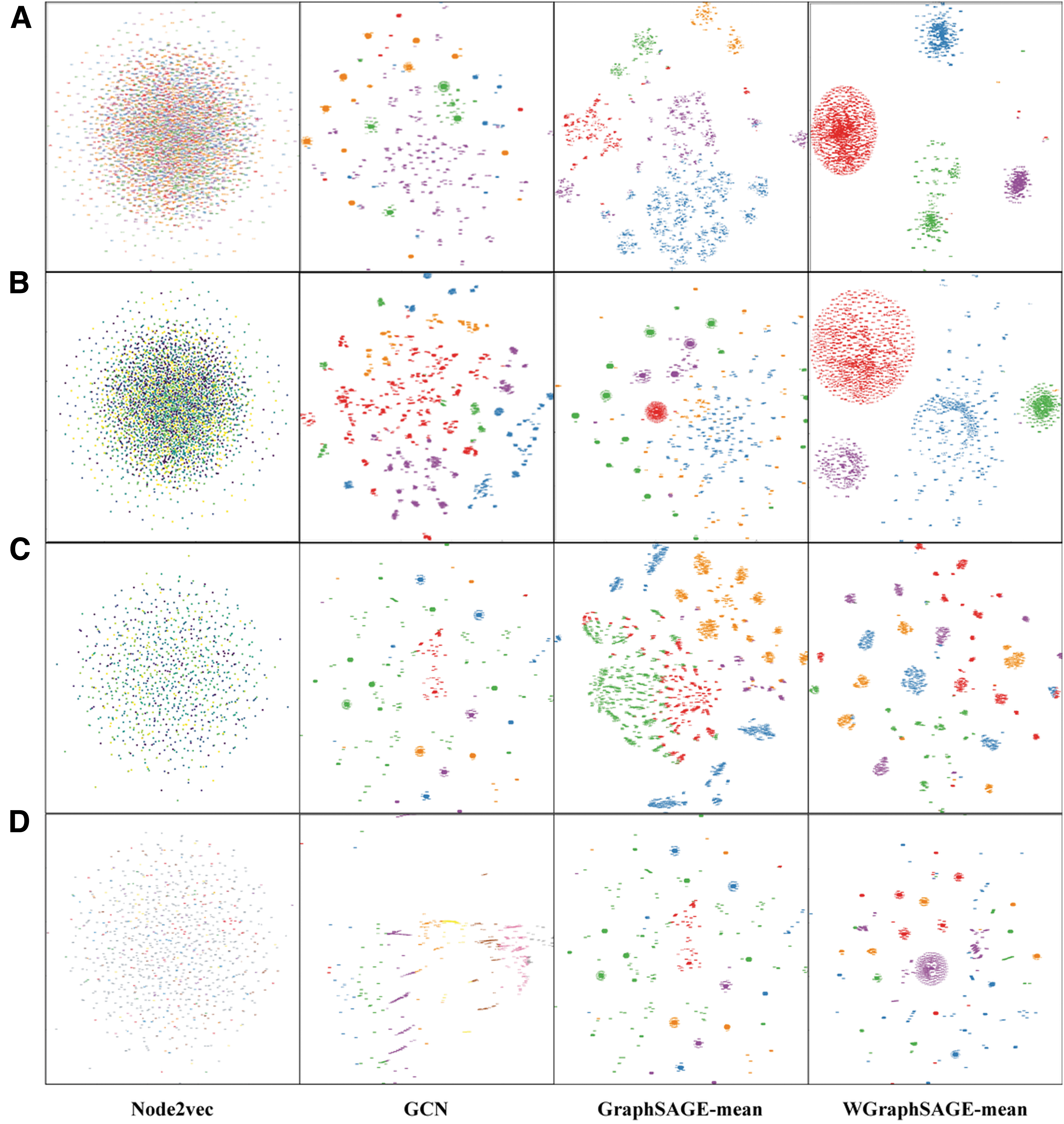
Clustering results.
Node2vec does not reflect the relationship between nodes and fails to perform clustering. GCN clusters the nodes, and the clusters are more dispersed (i.e., the distance between the clusters is large), but the distance within clusters is large and there are too many clusters. As for the clustering results of GraphSAGE, the number of clusters is significantly reduced with smaller intracluster spacing, but the distance between clusters is small, which is not good for distinguishing different context scenarios.
WGraphSAGE achieves a significantly better aggregation effect than Node2vec, GCN, and GraphSAGE models, with a smaller intracluster distance, a larger distance between clusters, and an appropriate number of clusters. This result indicates that after weighted neighbor sampling and weighted aggregation by WGraphSAGE, the embedding information of graph nodes can better characterize the access records and reflect the relationship between them. Meanwhile, the associated nodes can be better clustered, and the clusters composed of these nodes correspond to the relevant context scenario information. Thus, the WGraphSAGE model proposed in this article achieves the modeling of context information and inference of context scenarios.
CAAC experiments
First, CAAC rules are developed for each of the four data sets. For the same data set, the OntCAAC and FB-CAAC models generate more rules than the WGraphSAGE model, as shown in Figure 8A. This is because the baseline methods OntCAAC and FB-CAAC use the ontology approach to develop rules manually, and there are more redundant rules. In contrast, the WGraphSAGE model automatically generates CAAC rules from the clustering results, which reduces the amount of redundant information.
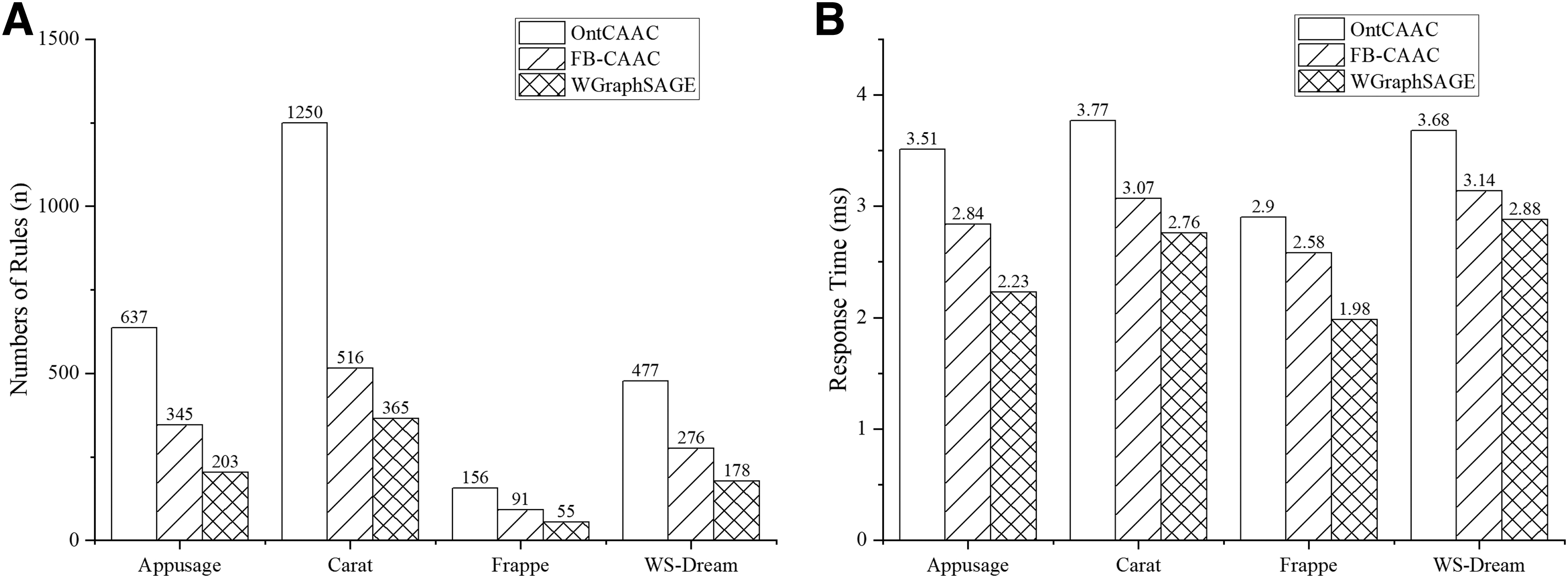
Access control decision results. For the same data set, the OntCAAC and FB-CAAC models generate more rules than the WGraphSAGE model, as shown in
Second, the generated rules are used to make control decisions on user access. In this article, the test data portion of the data set is used as a simulated access request to test the total response time when the system receives the access request to generate the access control decision. The decision response time is the sum of the context-aware time (Tca) and the access control rule matching time (Tacm), ignoring the network transmission delay. The OntCAAC, FB-CAAC, and WGraphSAGE methods were tested on each of the four data sets, respectively. The experiments compare the access control response time, and the test results are presented in Figure 8B.
The experiment results show that the response time of the access control decision of the WGraphSAGE method is significantly lower than that of other models. On the one hand, the rules have been generated by the context-aware approach before the WGraphSAGE model makes the access control decision. Its Tca is equal to the time to transform the access control request into a context information feature vector, which is much less than the time of the other two baseline models. On the other hand, the access control rule matching process of the WGraphSAGE model is essentially selecting the central node with the shortest distance. This time (Tacm) is the time to calculate the distance between the request vector and each clustering center node feature vector and rank them.
The experiment results indicate that the Tacm of the WGraphSAGE model is almost the same as that of the two baseline methods. In addition, the number of access control rules of the WGraphSAGE model is less than that of the baseline method, which reduces the number of rule matching. Therefore, the response time of the access control decision of the WGraphSAGE model is less than that of the two baseline methods.
Ablation experiments
To realize automatic context-awareness and automatic context relationship modeling and reasoning faced by big data access control, a new GNN model WGraphSAGE based on the baseline method GraphSAGE is proposed with weighted neighbor sampling and weighted aggregation algorithms. The importance of weighted neighbor sampling and weighted aggregation methods for the WGraphSAGE model and their roles in access control is verified by ablation experiments.
In the ablation experiments, four methods, GraphSAGE, GraphSAGE+WS, GraphSAGE+WA, and WGraphSAGE, are compared on four data sets for context-awareness and access control decisions. Figure 9A–D corresponds to the experimental results of the four data sets of Appusage, Carat, Frappe, and WS-Dream, respectively. GraphSAGE+WS represents the GraphSAGE model integrated with the weighted neighbor sampling method but without the weighted aggregation method. GraphSAGE+WA represents the GraphSAGE model still using the original random neighbor sampling method but adding the weighted aggregation method. SIL and DBI represent the evaluation metrics of the clustering effect of each model. “Numbers of Rules” represents the number of access control rules automatically generated by each model from the context clusters. “Response Time” represents the response time of each model to make access control decisions.
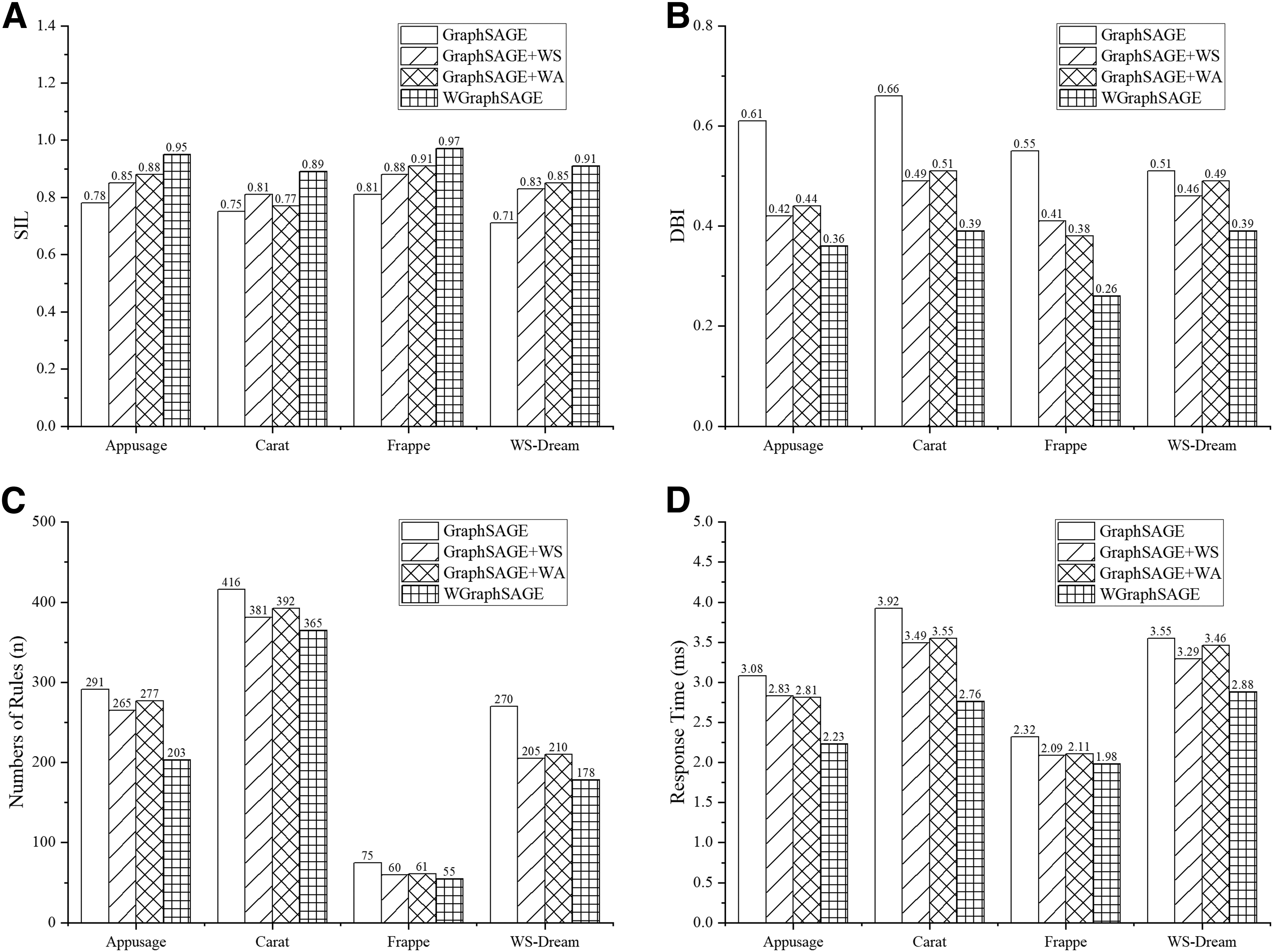
Analysis of ablation experiments.
The experiment results indicate that the WGraphSAGE model achieves the best results for each metric in the experiments on the four data sets. Adding only one of the methods of weighted neighbor sampling or weighted aggregation to the original GraphSAGE model, the clustering effect and access control results are better than those of the original GraphSAGE model but significantly worse than those of the WGraphSAGE model. For example, GraphSAGE+WS and GraphSAGE+WA are trained and tested on four data sets, and the experimental results of DBI, Numbers of Rules, and Response Time are higher than those of WGraphSAGE, and the results of SIL metrics are lower than those of WGraphSAGE.
The results of the ablation experiments show that the weighted neighbor sampling and weighted aggregation methods in the WGraphSAGE model play an important role in context information clustering and access control decision, which improve the effect of context awareness on the target data set and the efficiency of context-awareness access control.
Conclusion
This article aims at the problem that existing CAAC models cannot automatically context awareness and reason about context relationships. To this end, a context-aware approach based on a weighted GNN called WGraphSAGE is proposed, and a weighted neighbor sampling algorithm and a weighted aggregation algorithm are designed. Based on this, the CAAC rules are automatically generated by learning and reasoning about context scenarios and their relationships. The experiment results indicate that the proposed method has obvious advantages over the baseline method in automatic context awareness, context relationship modeling and reasoning, and dynamic access control. In future research, we will optimize the WGraphSAGE model to improve the resistance to noise and investigate model interpretability.
Footnotes
Acknowledgments
The authors would like to thank the editor and the anonymous reviewers for providing constructive and generous feedback.
Author Disclosure Statement
No competing financial interests exist.
Funding Information
This research was funded by the National Key Research and Development Program of China (No. 2018YFB0803603 and No. 2016YFB0501904) and the National Natural Science Foundation of China (No. 62102449).