Optimizing Multilayer Networks Through Time-Dependent Decision-Making: A Comparative Study

Abstract

This research highlights the importance of accurately analyzing real-world multilayer network problems and introduces effective solutions. Whether simulating protein–protein network, transportation network, or a social network, representation and analysis over these networks are crucial. Multilayer networks, that contain added layers, may undergo dynamic transformations over time akin to single-layer networks that experience changes over time. These dynamic networks, that expand and contract, can be optimized by guidance from human operators if the transient changes are known and can be controlled. For the expansion and contraction of networks, this study introduces two distinct algorithms designed to make optimal decisions across dynamic changes of a multilayer network. The main strategy is to minimize the standard deviation across betweenness centrality of the edges in a complex network. The approaches we introduce incorporate diverse constraints into a multilayer weighted network, probing the network’s expansion or contraction under various conditions represented as objective functions. The addition of changing of objective function enhances the model’s adaptability to solve a wide array of problem types. In this way, complex network structures representing real-world problems can be mathematically modeled which makes it easier to make informed decisions.

Introduction

The evolution of networks over time gives rise to dynamic networks.¹ This temporal change may exhibit a discernible pattern. For instance, hourly variations in the network topology of a vehicular traffic network offer insights into anticipated traffic conditions in subsequent hours.² Another study employed this network pattern in air transportation to analyze airport delays.³ With the advancement of robot technology, a robot searching over a region updates its current route upon encountering a barrier. However, the initially scanned region acts as a constraint for the next search space, preventing the robot from rescanning the same area. Due to the variability in the temporal network with each traverse, a new routing is necessary.⁴ Similarly, in dynamic graph coloring, re-optimization is performed by updating the search space with each graph refresh.⁵ In the context of disease spread within a community, the social network consists of individuals who have not contracted the disease, those who are infected, and those who have recovered. This social network undergoes changes over time based on the disease’s impact on individuals. Consequently, attempts have been made to control this dynamic change using reinforcement learning.⁶ In every scenario of how the network will take shape, emphasis is placed on the dynamic structure of the network. Various studies in the literature, including forecasting, classification, imputation, optimization, and anomaly detection, have addressed this dynamic network structure.⁷

The network structures mentioned above are important for comprehensively describing and analyzing complex systems across various disciplines. Within these systems, one can observe the presence of community structures, characterized by groups of nodes exhibiting denser connections among themselves compared with the rest of the network. This phenomenon is prevalent in real-world complex systems, including those in sociology, biology, transportation, and other domains.⁸ It is crucial for the network to accurately describe the relevant system, as an incorrectly constructed network can yield inaccurate results. Parameters such as the number of layers, node features, edge features, and transition weights between layers are all critical in system simulation. The construction of an elaborate network increases complexity, necessitating the subdivision of the network for thorough analysis. To achieve this simplification, a diverse range of methods is employed in clustering studies.^9–16 In a survey conducted by Huang et al., the methodological variances among the aforementioned studies were examined.¹⁷ In addition, there are also differences across application areas, such as biological clustering, social network clustering, and transportation clustering, among others.

Apart from the above-mentioned biological networks, transportation networks, social networks, it is possible to find layered network structures in supply chain problems. In Guo et al.,¹⁸ authors introduced different network layers based on various features, such as reviews and services that consumers share in online sales platforms. Our study also incorporates a multilayer network structure. In the next section, recent studies on multilayer dynamic networks, the methods used for network analysis, and the decision-making processes in these networks after analysis are examined. The rationale for such our study is also explained. The “Methodology” section provides detailed information about the algorithms, including the solver and objective function. In the “Experiments” section, we present schematics illustrating how the network evolves in different scenarios, along with the corresponding results. The “Future Directions” section discusses the significance of these findings, and the final section explores potential applications of our work.

Related Work

In this section, the literature on the use of multilayer networks is discussed. We will divide the discussion into multiple subsections, each focusing on different domains. Since different domains use different terminology where applicable we will consolidate them into the same terminology.

Multilayer structures on medicine network

In order to understand the complex network structures of proteins, especially in the biology field, images that cannot be accessed with a microscope are schematized with the help of various tools. We note that the majority of the structures used in this field are not dynamic but are multilayered in nature. In three-dimensional (3D) protein structures, NEMO and subsequently Alphafold2 have made significant progress in recovering and visualizing the helical structure of proteins, although not with high precision.^19,20 The helical structure helps generate information about the molecular structure of the peptide and its binding sites. These 3D structures are generated by predicting node diversity through protein–protein interaction (PPI), such as layer–layer interactions, determining connection threshold values, and outlining the topology of the protein structure. Following this process, multilayer clustering is employed, and the adjacency matrix of the network is constructed. Finally, functional enrichment can be applied to protein clusters, offering insights into their biological significance.²¹ Given the robust design of these 3D structures, some real biological networks have been observed to exhibit similarities with log-normal distributions.²² As an outcome of this approach, in biomedical bipartite networks, potential link connections, such as cancer occurrence, were predicted.²³

Layered networks serve as a computational tool not only in protein structure analysis but also in neuroscience and drug production, enhancing the functionality of numerous drugs. In addition, Pan et al.,²⁴ have demonstrated that multilayer networks effectively differentiate between individuals with mild cognitive impairment and healthy participants in Alzheimer’s disease classification tasks. Kurmukov et al.,²⁵ have proposed a framework for comparing both overlapping and nonoverlapping ensemble structures of brain networks that can be considered multilayer (one layer per lobe) using machine learning. Their findings emphasize the importance of pharmacology network construction in establishing an effective defense force in drug manufacturing.²⁶

Multilayer structures on transportation networks

Transportation networks have evolved into layered systems due to the growing variety of transportation modes in cities. The literature on transportation networks addresses a diverse range of issues, including road traffic flow, road origin-destination flow (for taxi, bike, e-scooter, ride-hailing), station-level subway passenger flow, station-level bus passenger flow, station-level shared vehicle flow, road traffic speed, road travel time, traffic congestion, vehicle demand, and traffic accidents.²⁷ This diversity of transportation modes underscores the complexity of urban land transportation. Aleta et al.’s²⁸ study focused on urban transportation in six distinct European cities. Simulations were conducted using three different layers, comprising tram, metro, and buses. In addition, two alternative layers, consisting of tram lines and bus lines, were employed for simulations in three other cities. In logistics transportation, which is characterized by a multimodal design, the transfer of products between modes is conceptualized as a multilayer network.²⁹ Similarly, the air transportation network is structured as a multilayered system and has been compared with ANGEL BINBALL and STARGEN models.³⁰ This multilayered network configuration arises from the diversity in aircraft, companies, and aircraft capacities. In cities facing escalating vehicular traffic, implementing multilayer networks can elevate the average transportation speed within the city.³¹ Therefore, designing transportation networks with multiple layers appears to be a pragmatic choice for addressing potential challenges in both research areas and city design.

Multilayer structures on communication and social networks

Social networks examine friendships, kinships, or professional ties, exploring the fabric of human connections by considering relationships and interactions. Communication networks investigate the flow of information and channels of communication within societies, focusing on the infrastructure that enables communication to take place. As in transportation networks, speed is an important parameter in communication networks which has become indispensable in society.³² Communication typically extends across diverse communities, such as family, work, and friends with varying levels of intimacies. Analyzing these communities using network methods is essential.³³ In contrast to transportation networks, social networks focus on nodes that represent individuals. Analysis of the network to reveal groups and cliques in a community has become important for both single-layer and multilayer social network structures. A wide array of methods is employed to cluster nodes within a social network. Chunaev³⁴ compared 75 different methods for community detection in node-attributed social networks. Among the commonly used techniques are k-means, Louvain,⁹ spectral clustering, and nonnegative matrix factorization.³⁴ Louvain, which maximizes the modularity value to cluster a multilayered network, stands out as a frequently employed method.⁹ For assessing the cluster quality, Newman³⁵ introduced a modularity metric (measures the strength of the division of a network into modules). Symmetric relations within a system give rise to a diagonal matrix, resulting in the formation of a bipartite network. Clustering of large networks was achieved by devising a minimax lower bound (lower bound to distinguish between close probability distributions) over a class of bi-clustering problems for modularity.³⁶ The ideal number of clusters in the network was investigated as well as the ideal number of layers. The determination of the optimal number of layers was accomplished through modularity maximization.³⁷ Communities are formed through the coexistence of various features, such as age, gender, education, and economic status. In addition, the nature of relationships (e.g., close friendships, family ties, or professional connections) varies, contributing to the complexity of social networks. Consequently, social networks may contain a large number of node and edge features. Identifying the optimal number of features is crucial for improving clustering accuracy.³⁸ Dimensionality reduction techniques are employed to reduce the number of features,³⁹ thereby enhancing computational efficiency and enabling faster convergence to a solution.

However, real-life problems often contain exceptions, and in cases where relationships are not symmetric cluster structure emerges. The BRIM algorithm, proposed by Barber⁴⁰, measures cluster quality in such instances. Network clustering applications have been instrumental in solving various problems. For instance, a k-partite network between two lobes of the brain revealed a neurological feature related to Parkinson’s disease. Statistical methods employed confirmed the existence of a relationship.⁴¹ A weighted bipartite network was established between projection and personal recommendation, uncovering changes in the congruence of personal order importance ranking with the network based on the projection shape.⁴²

Communication remains a societal necessity and the means of communication used create similarly complex networks. The design of a station (router) in a mobile network has proven effective in reducing the operational cost of service delivery.⁴³ The security of growing communication networks due to the increasing need for communication will pose a separate problem. The vulnerability posed by cyberattacks has become a societal challenge. Specifically, for encryption processes, an ideal pattern has been devised for the topological coloring of dynamic networks.⁴⁴

Multilayer structures on supply chain and distribution networks

Supply chain and distribution networks are complex networks across countries and product lines. In a distribution network, nodes provide information to their neighbors while simultaneously facing decision-making situations from neighbors, resulting in a bilateral cluster relationship. In structures with bilateral relationships (networks), optimal distribution is organized.⁴⁵ The pursuit of improved clustering quality or enhanced correlation relationships with topology in these studies, and similar ones, underscores a desire for optimality. The quest for the ideal parameters within the network contributes to the augmentation of statistical relationships.

The layered structures presented in Figure 1 represent the relationships and components across different scientific disciplines in Figure 1. Gray arrows show the interlayer relationship and black arrows show the intralayer relationship. For instance, a telecommunication network can be divided into distinct layers such as telephone, internet, and satellite, each possessing its own unique components (nodes and edges).^47,47 In this context, the decision regarding which layer of a telecommunication network will be expanded constitutes a strategic choice that impacts the overall structure of the entire network. Similarly, individuals maintain their social relationships through various social network platforms, with each platform serving a specific type of relationship. Consequently, while individuals may connect with the same people on some platforms, such connections may not exist on others. This necessitates modeling each social media tool as a separate layer.⁴⁸ Biological systems also exhibit a multilayered structure. For example, the human body comprises multiple intermediate structures, ranging from the cellular level to protein structures and organ formation. This hierarchical organization serves as a significant example for modeling biological layers.⁴⁹ Financial systems, too, have a layered network structure, with various subprocesses such as borrowing, lending, and investing within the banking sector. The financial instruments (nodes and edges) utilized in each process (layer) may vary, or certain operations may not be applicable.⁵⁰ This variation can alter the number of layers within the network. In this regard, Figure 1 schematically represents a financial system network. Although these real-world examples share similarities in terms of fundamental network components (nodes, edges, and layers), each system exhibits distinct structural and functional characteristics, resulting in notable differences.

FIG. 1.

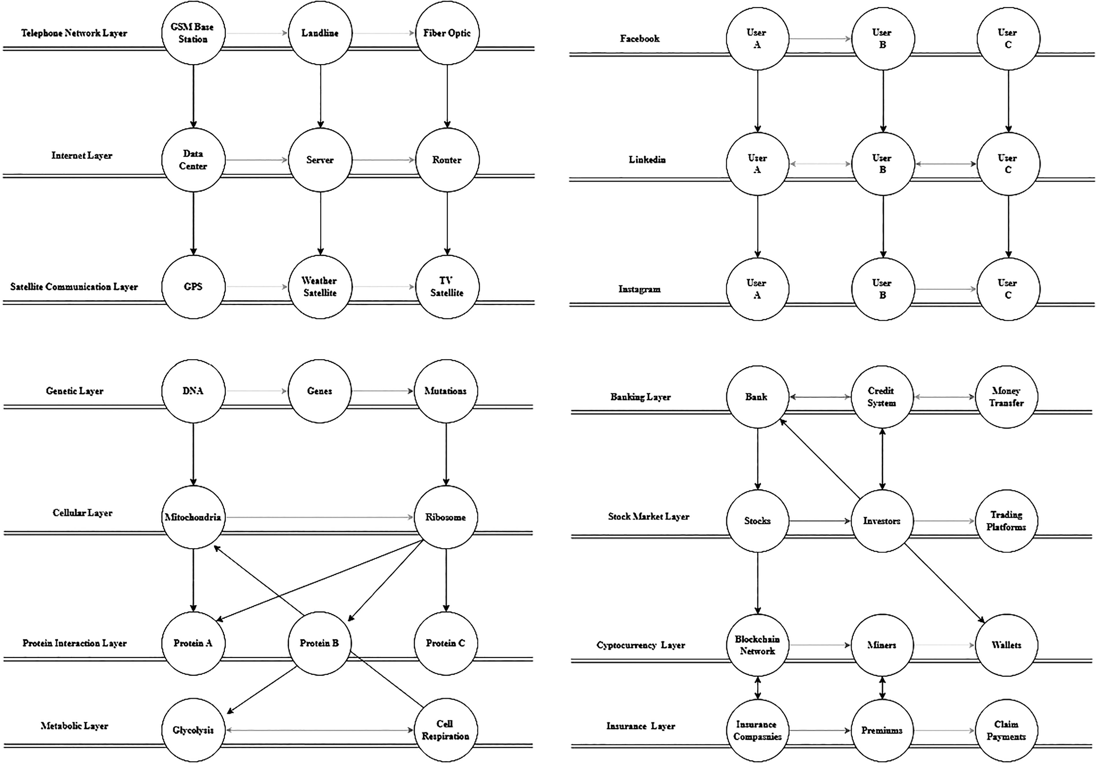
Schematic of multilayer networks used in different areas of life.

The complexity of the problem is heightened by the layered and dynamic nature of the network, a common challenge addressed in both the literature section and the studies presented here. Nearly all studies involve a process of network formation and subsequently analyzing the network. What sets our study apart from others is its ability to handle changes within a multilayered network under constraints defined by the users. The network in our framework can be weighted or unweighted, directed or undirected. Furthermore, depending on the nature of the problem, the network can be expanded or contracted within cost constraints. The motivations driving this research are twofold. First, it aims to fix the challenges of applied optimization on complex dynamic networks. This involves seamlessly integrating constraint generation and objective function generation processes into established graph software libraries, such as NetworkX (https://networkx.org). The second motivation is to develop a model capable of expanding or contracting complex networks based on the imposed constraints aligned with the specified objective functions. Our approach seeks to showcase the versatility of the proposed network modifications across diverse search spaces, ranging from biological networks to transportation and supply chain networks.

In the examples presented in this study, the betweenness centrality (EBC) metric has been utilized. This metric is a crucial measure for identifying different cluster formations within a network. It quantifies how frequently an edge is used in the shortest path selections. A higher frequency of usage for a particular edge leads to increased traffic on that connection. High traffic not only reduces the overall flow efficiency of the network but also increases its vulnerability. For instance, in an electrical circuit, excessive usage may result in overheating, whereas in a water pipeline network, increased pressure can lead to pipe deformation or leakage. In contrast, edges and nodes where the shortest path usage is more evenly distributed exhibit a lower risk of such failures.

By doing so, this research contributes to advancing the understanding and applicability of optimization techniques in dynamic environments across various domains.

Methodology

This section describes how to control a dynamic network in various scenarios in the case when the network is multilayer. The network can be weighted, directed, and undirected. It also contains constraints and changes in the objective function that may alter the optimal decision. The aim of the construction of our model is to be agnostic to the types of such multilayer networks. In addition, our model is designed to handle the expansion and contraction of the network, such as the addition and removal of nodes and edges.

Objective function and constraints

Our focus lies in examining the formation of a multilayer network concerning the objective function. As in a single-layer network, many metrics, such as EBC, can be computed in a multilayer network. Following this reasoning, one can arguably assume that multilayers are combined to present the network into a single layer and the metric values of the network can be subsequently measured from this single layer. This treatment, however, introduces significant errors as the interconnections between multilayers and within layers may not be uniform. Consider a transportation network, where the upper layer is defined by asphalt roads, while the lower layer is defined by rail and metro systems. The transition between the highway and subway often involves stairs, elevators, and walking. In another example, the bidirectional flow between roots and leaves of a plant (xylem and phloem) does not occur through the same material flow. Different minerals are transported from the root layer to the leaf layer, while distinct products move from the leaf to the root. Thus, in real-world scenarios, even the transitions between layers may carry different edge weights.

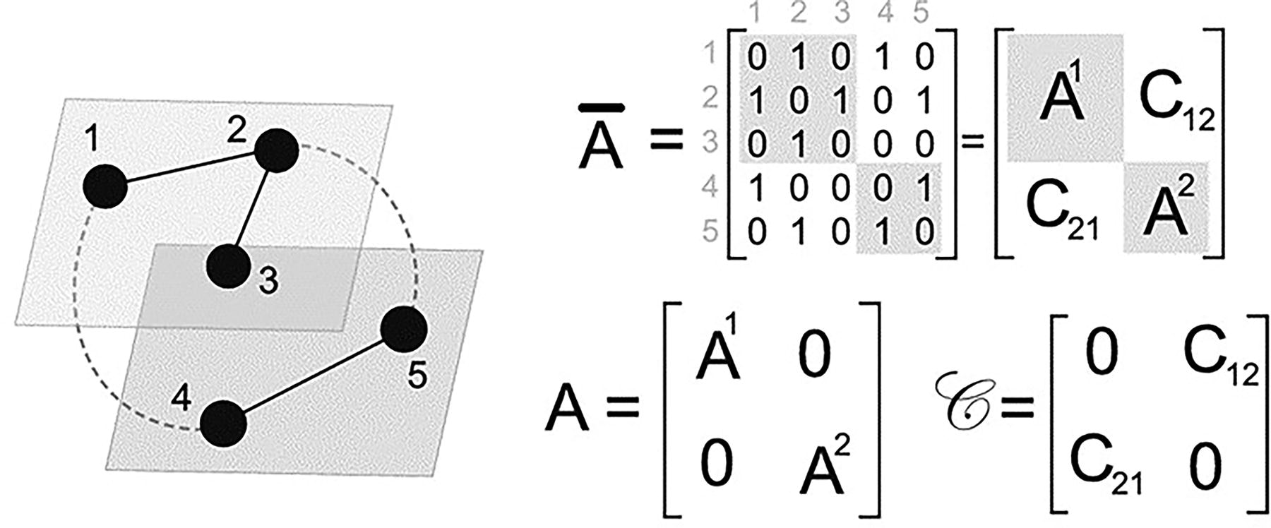
In multilayer networks, the adjacency matrix, which is used to calculate graph metrics, is interpreted as a supra-adjacency matrix in the context of a multilayer network. This structure is illustrated in Figure 2, where the connections both between and within layers are represented differently in the matrix.⁵¹ The supra-adjacency matrix of the MLN in Figure 2 is shown as $\bar{A}$ , where $A^{1}$ is the upper layer, $A^{2}$ is the lower layer, $C_{12}$ is the transition from the upper layer to the lower layer, and $C_{21}$ is the transition from the lower layer to the upper layer. Accordingly, matrix A represents intralayer connections while matrix G represents interlayer connections.

FIG. 2.

Formation of the supra-adjacency matrix for MLN.⁵¹

To calculate centrality values such as eigenvector centrality and Katz centrality in a multilayer network, the computation is performed using $\bar{A}$ matrix in Figure 2, utilizing the supra-adjacency matrix. However, when assessing EBC, it becomes necessary to compute the standard deviation (SD) which introduces complexity to the multilayer network. For instance, in a transportation scenario, a commuter traveling from home to work might opt to use either the highway (upper layer) or the metro (lower layer). For longer distances, the subway might be the preferred choice, whereas, for shorter distances, it might not be as practical due to the potential time spent in transit between layers. Consider, for example, that 10 additional minutes for this transfer could accumulate to a total of 20 minutes (since there will be two transfers such as $C_{12}$ and $C_{21}$ between the two layers). Consequently, for short-distance travel, changing layers may not be economic. Calculating the shortest path (SP) routes within this multilayer network further amplifies the complexity of the problem.

As a case study, distinct SP values were computed for interlayer and intralayer scenarios, and the EBC for a two-layer network was determined using the following equations: $A = (\sum_{α \in L_{1}} \frac{σ_{i^{a} j^{a}}^{v^{u}}}{σ_{i^{a} j^{a}}} + \sum_{β \in L_{2}} \frac{σ_{i^{β} j^{β}}^{v^{u}}}{σ_{i^{β} j^{β}}})$ (1) $B = (\sum_{α \in L_{1} : β \in L_{2}} \frac{σ_{i^{a} j^{β}}^{v^{u}}}{σ_{i^{a} j^{β}}} + \sum_{α \in L_{1} : β \in L_{2}} \frac{σ_{i^{β} j^{α}}^{v^{u}}}{σ_{i^{β} j^{α}}})$ (2) $C^{(v^{u})} = \sum_{i, j \in V : i \neq j} (δ A + (1 - δ) B)$ (3)

The $α$ in Equations 1 and 2 assumes various values depending on the transition between intra and interlayers. Selecting the ratio that most accurately models the problem at hand will yield more reliable and consistent solutions. In Equation 3, $C^{(v^{u})}$ represents the centrality value of vertex $v$ in layer $u (a$ or $B$ ). $δ$ is the layer weight of the links within each layer in the intralayer, while $(1 - δ)$ represents the weight of the links in the interlayer. The SP algorithm will yield distinct routes and, consequently, different edge values depending on whether it is applied in the interlayer or intralayer context. $σ_{i^{a} j^{a}}^{v^{u}}$ indicates whether the edge $v$ in layer $a$ lies or does not lie on the SP route between $i$ and $j$ , whereas $σ_{i^{a} j^{a}}^{v^{u}}$ denotes the SP between $i$ and $j$ . In this scenario, $α$ and $β$ represent two distinct layers. If the transition weights from $α$ to $β$ and from $β$ to $α$ are unequal, it will be necessary to assign different weights for these two cases based on the nature of the problem. $σ_{i^{a} β}^{v^{u}}$ s is the state of an edge $v$ in layer $u$ on the SP route at a transition between layers. $σ_{i^{a} j^{β}}$ is the SP route between these layers ( $i$ and $j$ are in different layers). Therefore, $\forall u$ the edges in each layer are examined, and $u$ consists of $a$ and $β$ for a two-layer network. For ease of solution, transition edges have been assigned to layer $a$ or $β$ ; therefore, the set $u$ covers all edges.

This study focuses on four different problem scenarios: -

(S1) Minimize the SD between the EBC values in the whole system by adding edges to only one layer in a multilayer network.

(S2) Minimize the SD between the EBC values in the other layer by adding edges to only one layer in a multilayer network.

(S3) Minimize the SD between the EBC values in the whole system by subtracting edges in only one layer in a multilayer network.

(S4) Minimize the SD between the EBC values in the other layer by subtracting an edge in only one layer in a multilayer network.

Below is a mathematical model designed for expanding or contracting a multilayer network. While this model provides an optimal solution for our case study, these solutions are identical to the heuristic approach.

Indies

$i, j, k, l$ Represent each node in the existing network.

$t$ Represents time and is binary (0 or 1) in this model.

$u$ Represents layer names in a two-layer network, denoted as $a and β$ .

(′) represents edges that do not exist in the network at time 0.

Parameters

$w_{ijt}$ Cost determined for edge (i, j) at time t.

$a$ The total number of edges in the network at time 0.

$b^{adding}$ Number of edges to be added to the network.

$b^{removing}$ Number of edges to be removed from the network.

Set of nodes.

${A_{ijt}}^{u}$ EBC value of intralayer calculated for edges (i, j) in each layer u at time t.

${B_{ijt}}^{u}$ EBC value of interlayer calculated for edges (i, j) in the routing between layers u at time t.

$C^{({v_{ijt}}^{u})}$ Generic EBC values calculated for edges (i, j) at time t in the u layer network.

$δ C^{({v_{ijt}}^{u})}$ Ratio that determines the weights of intra- and inter-EBC values to calculation of generic EBC.

$\bar{C}$ Average of the EBC in a multilayer network.

$σ (i, j)$ The number of SPs between points i and j.

$σ (i^{u}, j^{u^{'}})$ The number of SPs between points i and j across different layers u is represented by a binary variable (0 or 1).

${v_{ij 0}}^{u}$ * Edge (i, j) existing in the network at time 0. While this variable is a fixed parameter in the case of expanding the network, it is a decision variable in the case of narrowing the network. Because which edges to be removed are searched in this sample space.

${v'}_{ij 0}$ * Edge (i, j) that does not exist in the network at time 0. This variable is a fixed parameter in the case of network shrinkage, while it becomes a decision variable in the case of network growth. Because which edges to add are searched in this sample space.

Decision variable

${v_{ijt}}^{u}_{inter}$ The state at time t whether or not an edge (i, j) in layer u in the network is on the SP in any route. ${v_{ijt}}^{u}_{inter}$ is binary (0 or 1) variable.

${v_{ijt}}^{u}_{intra}$ At time t, whether or not the edge (i, j) in the network is in the SP in any route between layers u. ${v_{ijt}}^{u}_{intra}$ is binary (0 or 1) variable.

$Y$ Binary 0 or 1 variable created for the “either or” constraint.

${v_{ij 1}}^{u}$ Indicates whether there will be an edge (i, j) in the network from time 0 to time 1. ${v_{ij 1}}^{u}$

Mathematical model

Min z = \sqrt{\frac{1}{N} \sum_{i = 0}^{N} \sum_{j = 0}^{N} \sum_{u = α}^{U} {(C}^{({v_{i j 1}}^{u})} - \bar{C})^{2}}

(4)

Subject to: ${A_{i j 1}}^{u} {v_{i j 1}}^{u}_{intra} - \frac{\sum_{k \neq l} i f {\begin{matrix} {1, argMin}_{sub} ({v_{i j 1}}^{u}_{intra}) \in {σ (k, l)}^{u} \\ {0, argMin}_{sub} ({v_{i j 1}}^{u}_{intra}) \notin {σ (k, l)}^{u} \end{matrix}}{\sum_{k \neq l and (k, l) \neq (i, j)} 1} = 0 \forall i, j, u$ (5) ${B_{i j 1}}^{u} {v_{i j 1}}^{u}_{inter} - \frac{\sum_{k \neq l} i f {\begin{matrix} {1, argMin}_{sub} ({v_{i j 1}}^{u}_{inter}) \in σ (k^{u}, l^{u'}) \\ {0, argMin}_{sub} ({v_{i j 1}}^{u}_{inter}) \notin σ (k^{u}, l^{u'}) \end{matrix}}{\sum_{k \neq l and (k, l) \neq (i, j)} 1} = 0 \forall i, j, u$ (6) $C^{({v_{i j 1}}^{u})} - (δ {A_{i j 1}}^{u} + (1 - δ) {B_{i j 1}}^{u}) = 0 \forall i, j, u$ (7) $\bar{C} - \frac{\sum_{i = 0}^{N} \sum_{j = 0}^{N} \sum_{u = α}^{U} C^{({v_{i j 1}}^{u})} {v_{i j 1}}^{u}}{\sum_{i = 0}^{N} \sum_{j = 0}^{N} \sum_{u = α}^{U} {v_{i j 1}}^{u}} = 0$ (8) $If \{\begin{matrix} \sum_{i = 0}^{N} \sum_{j = 0}^{N} \sum_{u = α}^{U} {v^{}'}_{i j 0}^{u} \leq b^{adding} \\ o r \\ \sum_{i = 0}^{N} \sum_{j = 0}^{N} \sum_{u = α}^{U} {v_{i j 0}}^{u} \leq {a - b}^{removing} \end{matrix}$ (9) ${v_{i j 0}}^{u} + {v'}_{i j 0}^{u} - {v_{i j 1}}^{u} = 0 \forall i, j, u$ (10)

Model intralayer SP ${Min}_{intra} \sum_{u = a}^{U} \sum_{i = 1}^{N} \sum_{j = 1}^{N} w_{i j 1} {v_{i j 1}}^{u}$ (11)

Subject to: $\sum_{i = 1}^{N} \sum_{j = 1}^{N} {v_{i j 1}}^{u} - \sum_{i = 1}^{N} \sum_{j = 1}^{N} {v_{j i 1}}^{u} \{\begin{matrix} 1, i (source node) \\ - 1, j (target node) \\ 0, others \end{matrix} \forall u$ (12)

Model interlayer SP ${Min}_{inter} \sum_{u = a}^{U} \sum_{i = 1}^{N} \sum_{j = 1}^{N} w_{i j 1} {v_{i j 1}}^{u}$ (13)

Subject to: $\sum_{u = a}^{U} \sum_{i = 1}^{N} \sum_{j = 1}^{N} {v_{i j 1}}^{u} - \sum_{u = a}^{U} \sum_{i = 1}^{N} \sum_{j = 1}^{N} {v_{j i 1}}^{u} \{\begin{matrix} 1, i (source node) \\ - 1, j (target node) \\ 0, others \end{matrix}$ (14) ${Y (v_{k j 1}}^{a} + {v_{i l 1}}^{β} - 2) \leq 0$ (15) ${(1 - Y) (v_{k j 1}}^{β} + {v_{i l 1}}^{a} - 2) \leq 0$ (16) ${v_{i j 1}}^{u}, {v_{i j 0}}^{u} *, {v'}_{i j 0}^{u} *, {v_{i j 1}}^{u}_{intra}, {v_{i j 1}}^{u}_{inter}, Y = {0, 1} \forall i, j, u$ (17)

Below is a mathematical model designed for expanding or contracting a multilayer network. While this model provides an optimal solution, it fails to find the optimal result as the number of nodes, edges, and layers in the network increases. In the above model, the equations from Equations 4 to 9 define the main mathematical model. In addition, Equations 10 and 11 represent a submodel referred to as “Model Intralayer SP,” while Equations 12 –15 correspond to another submodel called “Model Interlayer SP.” Equation 4 aims to minimize the SD of EBC values for all edges in the network, ensuring a balanced traffic load distribution across the edges. Equation 5 utilizes an “if” piecewise function within the Model Intralayer SP to determine whether each edge ${v_{i j 1}}^{u}$ belongs to the SP set for the (k, l) route. By computing the SP using the Model Intralayer SP, the set ${σ (k, l)}^{u}$ is formed for the (k, l) route. Consequently, the edge (i, j) is assigned a value of either 0 or 1 depending on whether it is included in this ${σ (k, l)}^{u}$ set. The value ${A_{i j 1}}^{u}$ is then determined based on the EBC for each edge (i, j) in layer u. Equation 6, on the other hand, constructs an SP set using $σ (k^{u}, l^{u'})$ considering scenarios where the start and end points of the (k, l) route are in different layers ( $u, u'$ ). The value ${B_{i j 1}}^{u}$ is computed based on the EBC values of the SPs within $σ (k^{u}, l^{u'})$ . Equation 7 derives a general EBC value for each edge by considering the intralayer and interlayer EBC values, weighted by the factor δ, highlighting the distinct traffic loads in intralayer and interlayer structures. Equation 8 calculates the average EBC value for the entire network based on the EBC values of all edges, which is crucial for SD computations. Equation 9 includes two distinct constraints: If the goal is to expand the network by adding an edge, the upper constraint is applied. If the goal is to reduce the network by removing edges, the lower constraint is used. The selection between these constraints depends on the type of the problem. Equation 10 models the transformation of edges over time by considering the existing edges ( ${v_{i j 0}}^{u}$ ) and candidate edges ( ${v'}_{i j 0}^{u}$ ) at time 0, which are then used to determine the edges ( ${v_{i j 1}}^{u}$ ) at time 1 based on model decisions. Equation 11 calculates the SP for each $v_{i j 1}$ edge within a specific route by considering its cost ( $w_{i j 1}$ ). Equation 12 consists of three constraints: The starting node of the route must have only one outgoing edge. The ending node must have only one incoming edge. Intermediate nodes must ensure a balance between incoming and outgoing edges. Since the start and end nodes are predetermined, a subtour constraint is not included. Equation 13 aims to find the SP between layers. Equation 14 assigns values of −1 and 1 to the entry and exit conditions at the start and end nodes while setting 0 for intermediate stations, where the inflow and outflow must be balanced. Equations 15 and 16 ensure that the start and end layers of the route between nodes k and l are distinct, thereby enabling the calculation of the interlayer SP value. The final constraint defines the assignment values (binary) of decision variables. This mathematical model is designed to optimize edge load balancing and manage topological changes in multilayer networks.

LP (Linear Programming) and MILP (Mixed-Integer Linear Programming) solvers (CPLEX, Gurobi, and Xpress) handle between 100,000 and 1,000,000 variables (www.gams.com). However, an increase in the number of constraints, the number of layers in the network, and having a dense network will reduce this number.⁵² For example, in a traffic network, each road may be assigned various features, such as the number of lanes, road type, slope, speed limit, proximity to hospitals, schools, shopping centers, population density, and the number of traffic lights.⁵³ An increase in the number of features assigned to a node or edge contributes to a more complex network structure, which in turn makes network analysis and solution development more challenging.

For a directed network consisting of only 1000 nodes, the number of edge options, that is, the solution space, is n (n − 1), resulting in 999,000 possible edges. Therefore, two different algorithms incorporating heuristic methods have been developed to address problem sizes that the above mathematical model is unable to solve. Algorithm 1, which is detailed below, is designed to address scenarios S1 and S2 and is depicted in Figure 3. For the last two scenarios (S3 and S4), Algorithm 2 which is detailed below has been devised and is presented in Figure 4. Rows 32–68 in Algorithm 1 encompass the constraints and objective functions. Newly generated edge options undergo eligibility checks before being incorporated into the existing network. If the same numbers are generated, the proposed two points may not form an edge. In addition, the proposed edge could already be included in the existing network set. To circumvent these scenarios, preemptive measures outlined between rows 40 and 45 in Algorithm 1 are implemented. The set of randomly generated edges is assigned to the “Edgelist” variable. At row 43, “Edgelist” is duplicated and named “UniqueEdgeList.” When “UniqueEdgeList” encounters a node (row 44 to row 45) or an edge assignment from the current network (row 42 to row 43), it drops these assignments from the current “UniqueEdgeList” set. Consequently, the cluster similarity associated with this “Edgelist” dissipates. If “EdgeList” and “UniqueEdgeList” do not match, the cost value will be set to $\infty$ . Consequently, Algorithm 1 will generate values contrary to the desired situation as the iterations progress. Constraints play a crucial role in this part of the algorithm. Given that the network is weighted, a weight is necessary for the proposed new edge to be meaningful. In other words, merely suggesting an edge is not sufficient to expand a weighted network. To address this, we introduce the $γ$ parameter. The SP value in the existing network between the two points forming the potential edge, when multiplied by the $γ$ constant, determines the weight value of the potential new edge. The $γ$ value is between 0 and 1. Taking into account that the potential new path will shorten the SP to a certain extent, a ratio of 0.7 (“г” in Algorithm 1) was chosen for this study. This value is arbitrarily set to 0.7. This value may vary depending on the nature of the real network. It is assumed that the SP distance before the new path decision taken will be 0.7 times shorter with the new path added. This ratio can be changed according to the problem definition. The selection of the ratio guarantees that the new edge will improve the existing route. In Algorithm 1, this weight assignment is determined in row 39, and in rows 47 and 48, an edge in the solution set is added to the network in the layer where the change will occur.

FIG. 3.

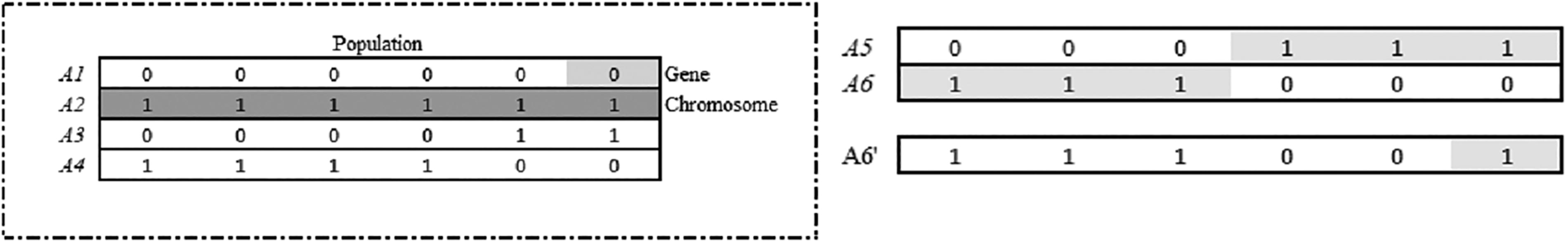
Basic genetic algorithm components and altering of a single gene.

FIG. 4.

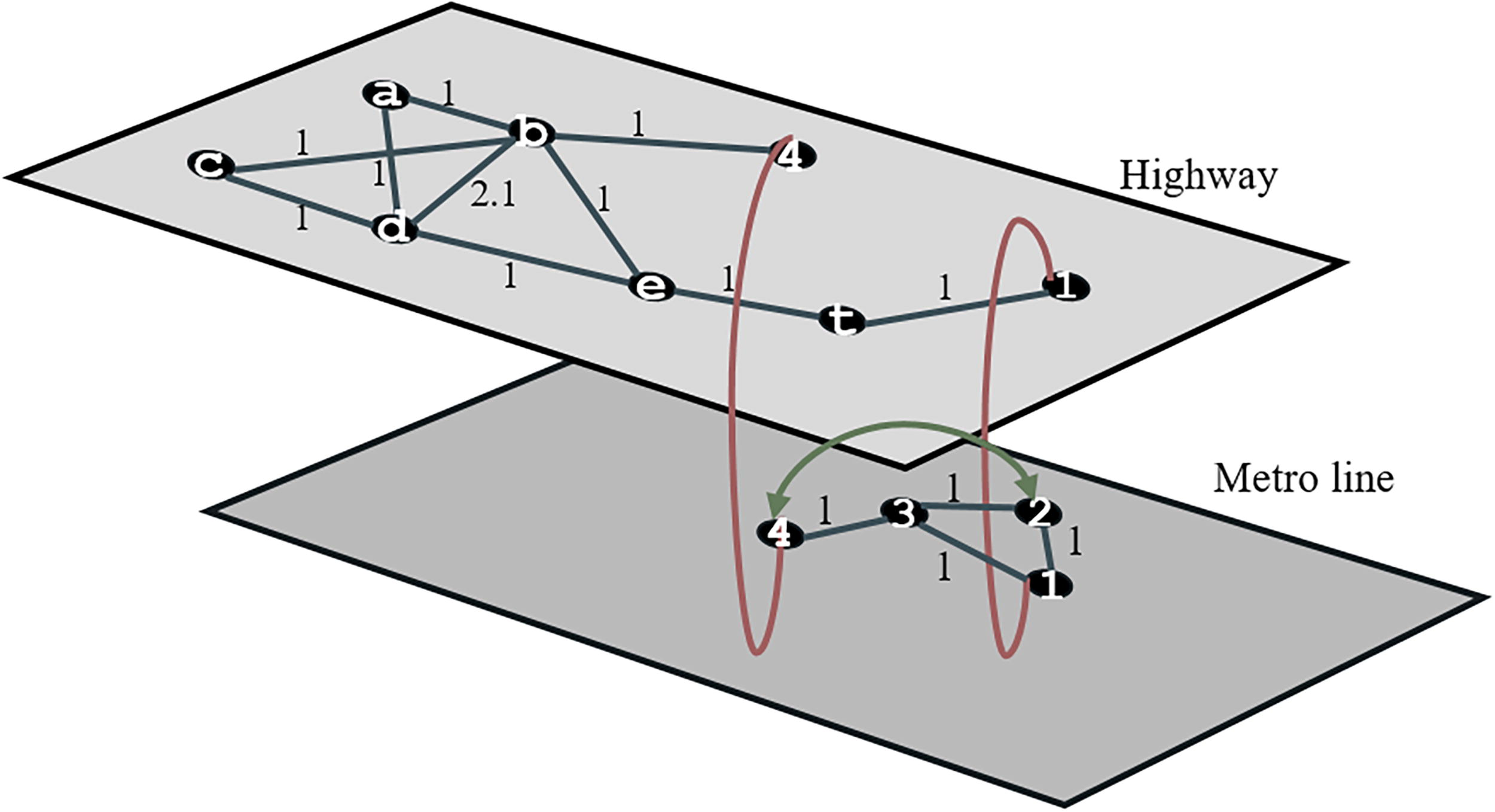
Weight multilayer directed network.

Next, in row 49, the updated layer is integrated into the entire system, preparing the multilayer network at time $T_{0}$ for time $T_{1}$ . Between rows 50 and 55, both the intralayer and interlayer EBC values of the network at time $T_{1}$ are computed. In row 52, the change of “i” and “j” is recorded to simulate a bidirectional transition. Subsequently, in row 56, ${EBC}_{(m l)}$ , representing the EBC values of the entire network, is calculated using Equation 3. For the first two questions mentioned earlier, two distinct costs are defined in rows 57 and 58. The cost in row 57 computes the SP between the edge values of the entire network, while the ${Cost}_{(alternative)}$ in row 58 calculates the SP between the EBC values of only the layer where no change has occurred. The objective in ${Cost}_{(alternative)}$ is, for instance, to reduce highway traffic, a critical aim of subway construction in a transportation network. When commuters prefer using the subway, the use of cars in the upper layer of the city diminishes. Consequently, shaping the subway system induces a density shift in the unaltered highway layer. Various variations can be employed in generating the cost function (objective function). For instance, one may solely compute the SP value between the updated network’s EBCs.

We design Algorithm 2 for answering the last two questions above. The algorithm is shown in Figure 4. If the network contracts by deleting an, the search space needs to be shaped over the edges of the existing network. Therefore, the constraints mentioned in Algorithm 1 are not included in the deletion algorithm. Randomly generated numbers only allow selection from the set of edges in the current network. Thus, there is no weight generation as in Algorithm 1. The objective function in Algorithm 2 is conditioned between rows 20 and 48. First, the number of edges to be deleted in the first 22 rows is indicated by the budget constraint. Selection is made according to the number of edges to be deleted. In row 32, the randomly selected edge is included in the “Edgelist.” In row 33, the edge or edges in the “Edgelist” are removed from the bt edge set at $T_{0}$ and a reduced edge set is created for time ${b t}_{t 1}$ . With this ${b t}_{t 1}$ set, first the ${B T}_{t 1}$ network is constructed in row 34 and then the ${M T}_{t 1}$ network is constructed by merging it with the unmodified ${U T}_{t 0}$ network. For the new graph, interlayer and intralayer EBC values are calculated in rows 42–44 just like in Algorithm 1. Then all EBC values of the network are calculated according to the г parameter according to the connection properties between the interlayer and intralayer. The г value was determined as 0.8 in this study. Two different cost variables are shown in Algorithm 2. These can either minimize the SD of the whole network or minimize the EBC distribution of only a particular layer. This choice can be implemented with different layer preferences depending on the type of problem. For this study, this preference is chosen as ${U T}_{t 0}$ (upper network).

In general, each initialization algorithm consists of an edge set representing the existing network and a candidate edge set for potential assignments. Algorithm 1 iteratively adds a new edge to the existing network within the given budget constraint and calculates the EBC of the updated network. However, before constructing a new network, the existing edge set and the candidate edge set are merged at a cluster level, enabling the dynamic formation of a new network at each step. This approach facilitates the integration of genetic algorithms with the NetworkX library. Similarly, in Algorithm 2, the existing edge set also represents the search space. Consequently, based on the allocated budget, certain edges are removed from this set, a new network is reconstructed, and the EBC value is recalculated.

Minimization algorithm

Algorithm 1 and 2 are described with four different objective functions and associated constraints. Within these constraints, a heuristic solver approach was employed to compute the objective function for complex and large-scale networks. Searching for the optimal solution in a mathematical model becomes exponentially complex as the network size grows. This can lead to difficulties in implementing the model. Hence, a genetic algorithm was adopted in this study. The choice of a genetic algorithm stems from its applicability to a wider range of problem types compared with other heuristic methods. Figure 3 illustrates the chromosome generation patterns required for the genetic algorithm to explore the solution space. Each row, represented by A1–A4 in Figure 3, signifies a chromosome. Every square within the chromosome represents a gene, and the four chromosomes (A1–A4) collectively form a population of four. Furthermore, rows A5 and A6 give rise to two distinct chromosomes through gene exchange, employing a half-and-half crossover of rows A1 and A2. In addition, a significant degree of diversity is introduced through mutation. The alteration of a single gene in chromosome A6 results in chromosome A6′.

Algorithm 1: Growth of a layer in a multilayer network to create a balanced network.

Algorithm 2: Shrinking edge at one layer in a multilayer network to create a balanced network.

In Algorithm 1, chromosome sets are generated from different gene sequences according to the budget constraint in row 23. These chromosome sets are referred to as the population (row 23). In the decoder section between rows 25 and 29, each chromosome is decoded and converted into an integer number. The pairs generated according to the budget constraint represent an edge. Before running the algorithm, the node names need to be converted into an ordered integer array to enable efficient searching of the search space. This transformation will facilitate the operation of the algorithm. To further illustrate this, let’s imagine that there is a trade relationship between three different countries. For example, in only a single-layer network representing a three-node relationship involving Germany, Turkey, and the UK, we can code the nodes as 1 (Germany), 2 (Turkey), and 3 (UK). This way, a search space between 1 and 3 is created. The 24th row in Algorithm 1 represents the number of times (number of iterations) the initially generated population set will be renewed. The crossing over and mutation steps in both algorithms ensure that different chromosomes are formed in each iteration. The best solution and the best network components of each iteration are memorized by the LBS (local best solution) and LBL (local best link) algorithms and compared with the better solutions that may occur later to reach the GBS (global best solution) and GBL (global best link) values. There is no difference between Algorithms 1 and 2 in the use of genetic algorithms except for the decoding part. In Algorithm 1, the links are generated, while in Algorithm 2, selections are made from the existing link set.

Experiments

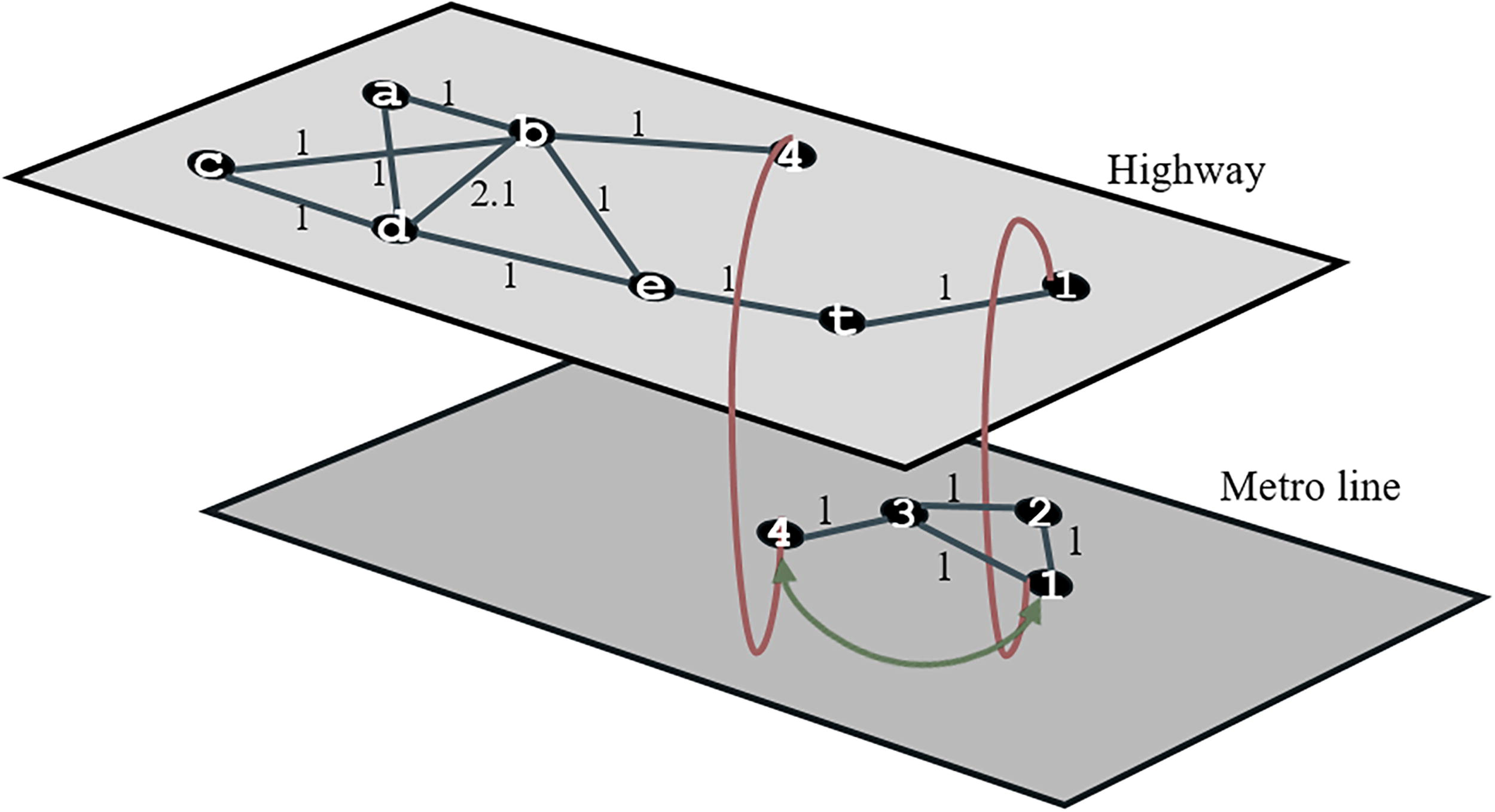
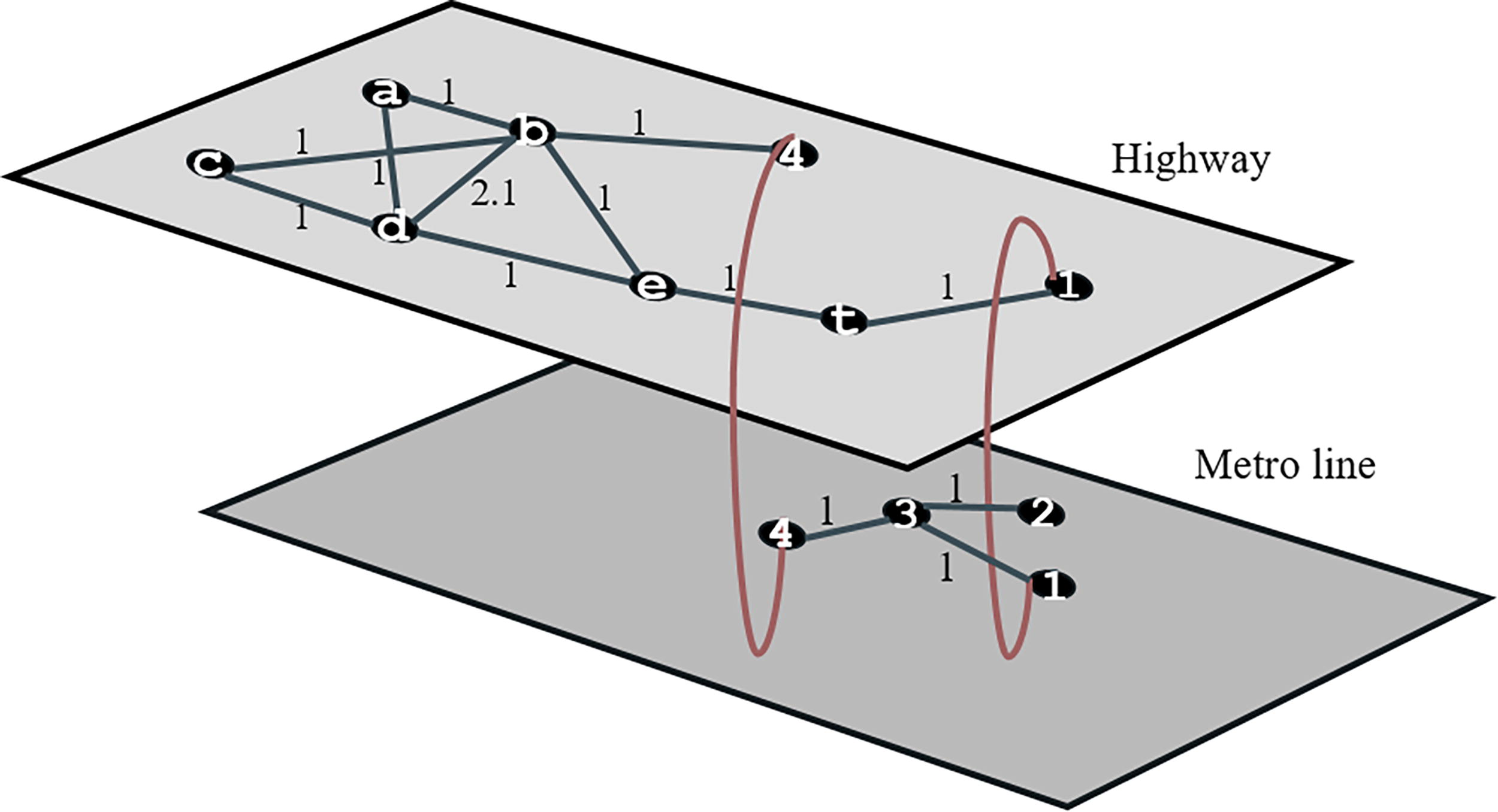
For four different scenarios outlined in the “Objective Function and Constraints” section, a simple network is designed and visualized in Figure 4. In this section, the networks were generated randomly. To facilitate the detection of network structures and potential changes, a limited number of layers, nodes, and edges were employed. This choice simplified the visualization of the network, making it more comprehensible and interpretable. In the network shown in Figure 4, the upper layer is designed as a highway network and the lower layer as a metro network. The network in the upper layer is designed as a weighted network due to the nature of the highway. The (d–b) edge is assigned a distance weight of 2.1, while the other links are assigned a different value. (b–4) edge and (1–t) edge symbolize a bidirectional transition between the layers. The edges symbolize transfer stations, especially in transportation networks. For the lower layer, equal travel times are assigned.

Both the means of transportation between the layers, the materials used for the infrastructure, and the capacity of the means of transportation have led to the formation of two different layers. A scenario was created in which a one-stop addition to the metro network would be made within the available resources. The EBC of each edge in the basic multilayer network at time $T_{0}$ (as shown in Fig. 4) is calculated according to Equation 3, and the SD between the values of the edges is 0.78. The highest EBC value in this network at time $T_{0}$ was found for edge (a–b). The г value for this measurement was set to 0.7. If the edge to be added to the lower layer is intended to balance the EBC in the entire network, this value was determined to be edge (2–4) according to Algorithm 1. Since the network is designed to be directional, edge (2–4) represents a one-way connection. The updated network is shown in Figure 5. Consequently, the SD of the EBC values between the edges of the multilayer network at time $T_{1}$ is found to be 0.75. Thus, a more balanced network is designed compared with the network at time $T_{0}$ .

FIG. 5.

The result produced by Algorithm 1 for the EBC balance between two layers. EBC, betweenness centrality.

The shaping of the network at $T_{0}$ can be modeled with a different objective function depending on the nature of the network and the type of problem. Namely, if the shaping of the metro network (lower layer) is to balance the vehicle traffic on the highway (upper layer), only the SD between the EBC values of the edges in the upper layer is minimized. After calculating the EBC values of the multilayer directed network in Figure 4, only the SD of the EBC values in the upper layer is calculated as 0.63. For the network in Figure 4, edge (1–4) was proposed by Algorithm 1, resulting in Figure 6. Since the network is designed to be directional, edge (1–4) represents a one-way connection. In Figure 4, when the SD between the EBC values of only the upper layer among the EBC values of the whole network is calculated, it is found to be 0.041. This value was obtained by subtracting the values of the upper layer edges from the EBC values of the multilayer network formed by updating the metro network at time $T_{1}$ . The SP value between the EBC values of the edge in this upper layer was found to be 0.59.

FIG. 6.

Only the result produced by Algorithm 1 for the EBC balance in the upper layer.

Considering the pedestrianization policies and revisions in city centers, the deletion of some edges in a multilayer undirected network is an option that decision makers may want to consider. Algorithm 2 is run on the network in Figure 4 for 1 and 2 edge deletion cases. The above two different scenarios (objection function) are applied for the edge deletion case. For 1 edge to be deleted, the results in Figure 7 were obtained by minimizing the SP values between the EBC values of the edges in the whole network.

FIG. 7.

The result deleted by Algorithm 2 for the EBC balance between two layers.

For both objective functions, the same results were obtained for the 1 and 2 edge deletion cases. In Figure 7, according to the network at $T_{0}$ , deleting edge (1, 2) results in an SD of 0.42 for the whole network and 0.37 for the upper network only. Considering that these values are 0.46 for the network at $T_{0}$ and 0.39 for the upper layer, it can be said that the possible deletion action will create an imbalance in the network. In addition, since the network is designed to be undirectional, edge (1, –2) represents a two-way connection.

Finally, Algorithms 1 and 2 were run separately for the scenario where two edges are deleted in the lower layer. For both objective functions, it is concluded that edges (2, 3) and (1, 2) are deleted. Since the network is designed to be undirectional, edges (1–2) and (2, 3) represent a two-way connection. The case where these edges are deleted is shown in Figure 8. In the network in Figure 8, the SD of the EBC of the whole network is 0.34, and the SD of the EBC of only the upper layer is 0.36. Considering that these values are 0.46 for the network at $T_{0}$ and 0.39 for the upper layer, it can be said that the possible deletion action will create an imbalance in the network.

FIG. 8.

Only the result deleted by Algorithm 2 for the EBC balance in the upper layer.

Table 1 shows the results of Algorithms 1 and 2 applied to directional and nondirectional networks in different scenarios and budgets. From this table, the approaches proposed in the study were found to provide overall improvement (a more balanced load distributed at the edges) for various types of networks.

Table 1.

Results generated for different scenarios for a multilayer network

Scenarios	Obj. function	Budget	Network type	$T_{0}$ network SD	Result	$T_{1}$ network SD
S1	Addition	1	Directed	0.78	(2, 4)	0.75
S2	Addition	1	Directed	0.63	(1, 4)	0.59
S3	Extraction	1	Undirected	0.46	(1, 2)	0.42
S4	Extraction	1	Undirected	0.39	(1, 2)	0.37
S3	Extraction	2	Undirected	0.46	(1, 2), (2, 3)	0.34
S4	Extraction	2	Undirected	0.39	(1, 2), (2, 3)	0.36

SD, standard deviation.

Conclusions

This study develops a control mechanism for various structures within a multilayer network. The complexity arises from the network being multilayered, featuring both directional and nondirectional variations, and incorporating weighted connections. In addition, the transition between layers exhibits varying densities, further complicating the network’s structure. Moreover, the growth of the network can target different objectives. Consequently, this study addresses these scenarios. Changes in weight parameters or structural elements of the network yield distinct outcomes. Particularly in multilayer networks centered around a primary layer, orchestrating formations in other layers to regulate processes in the main layer poses highly intricate challenges.

Future Directions

Multilayer networks have diverse application areas in biology, transportation, and social sciences. Subsequently, the algorithm proposed can be used on a number of problems: •

Planned alterations within any layer of a transportation network can be strategically designed.

•

Expansion and contraction in the flight route planning of airlines can be achieved.

•

It can facilitate cohesive planning across layers in pedestrianization studies.

•

Desired graphical changes can be orchestrated through the interaction of connections established by protein–protein networks for drug discovery.

•

Utilizing feature layers derived from customer feedback for product development, the product network necessary for marketing the ideal product can be devised.

•

Production planning can entail the redesign of supply chain networks.

Each of the topics mentioned above involves weighted or unweighted and directed or undirected networks, each with different objective functions, constraints, and varying numbers of layers. In essence, a new design seeks to modify the existing network structure. Therefore, for optimal design, the necessary constraints can be integrated into Algorithms 1 and 2 to guide decision-making across these complex networks. In this study, how to add constraints, how to update the complex network, and how to add the objective function were explained in detail for different problem types.

In this study, the EBC metric was utilized. However, the proposed approach can also be applied using different network metrics. For instance, metrics such as degree, eigenvector, closeness, and group centrality can be adapted to various problems and contexts, allowing for greater methodological diversity. In particular, closeness centrality can optimize the placement of stations in a transportation network, minimizing passenger travel times. Similarly, in a logistics network, it can be used to determine the optimal location for a new warehouse by minimizing its distance to other locations. Such a logistics network can be designed as a multilayered system, incorporating air, land, and sea transportation. On the other hand, group centrality can be an effective metric for identifying optimal router locations in a telecommunication network. As data traffic and connectivity demands increase in a given region, the placement of new routers can be optimized using the group centrality metric. If the network consists of wireless connections in certain areas and physical cable infrastructure in others, the system will evolve into a multilayered network structure. Therefore, the algorithms proposed in this study should not be limited to the EBC metric alone. Instead, the appropriate network metric should be selected based on the specific problem type. This approach ensures a more balanced metric distribution within the network and enhances the adaptability of the solution to different types of networks. In addition, no features have been assigned to network edges in this study. By incorporating feature assignments to edges or nodes, optimization processes can be developed for more complex network structures.

Limitation

The primary motivation of this study was to design a theoretical model; therefore, the proposed model’s solution times were not the focus of the analysis. For larger traffic networks or energy networks, real-world case studies can be used to evaluate and discuss solution times. This would allow for further optimization of the shared code, making it more efficient and applicable to practical scenarios.

Footnotes

Authors’ Contributions

K.M.: Contributed significantly to data collection and analysis, took a leading role in the design and writing of the article, contributed to the literature review and analysis, and made important edits during the writing process of the article. A.Y.: Played an important role in the idea development phase of the article, made significant contributions to the writing process, and also actively participated in the directed criticism and revision of the article, thereby improving the quality of the final version; in addition, also contributed significantly to the critical revision and editing of the article.

Data Availability

The dataset used in the study is open source and the study complies with ethical rules. The coding and dataset can be accessed from “” as open source.

Author Disclosure Statement

The authors declare that they have no competing interests. Ethical approval and consent to participate are not applicable. Consent for publication of all data contained in the article have been obtained from all authors. This research does not involve human participants and/or animals.

Funding Information

This study has not received any funding.

Abbreviations Used

References

Erlebach

, Hoffmann

, Kammer

. On temporal graph exploration. Journal of Computer and System Sciences, 2021; 119:1–18.

Bao

, Yang

, Zeng

. Graph to sequence learning with attention mechanism for network-wide multi-step-ahead flight delay prediction. Transportation Research Part C: Emerging Technologies, 2021; 130:103323.

Kang

, Yang

, Shan

, et al. Exploring Delay Propagation Causality in Various Airport Networks with Attention-Weighted Recurrent Graph Convolution Method. Aerospace, 2023; 10(5):453.

Khalidi

, Gujarathi

, Saha

. T: A heuristic search based path planning algorithm for temporal logic specifications. In 2020 IEEE International Conference on Robotics and Automation (ICRA). IEEE; 2020, pp. 8476–8482.

Bossek

, Neumann

, Peng

, et al. Runtime analysis of randomized search heuristics for dynamic graph coloring. In Proceedings of the Genetic and Evolutionary Computation Conference. ACM; 2019, pp. 1443–1451.

Meirom

, Maron

, Mannor

, et al. Controlling graph dynamics with reinforcement learning and graph neural networks. In: International Conference on Machine Learning. PMLR; 2021, pp. 7565–7577.

Jin

, Koh

, Wen

, et al. A survey on graph neural networks for time series: Forecasting, classification, imputation, and anomaly detection. arXiv Preprint, 2023; arXiv:2307.03759.

Newman

. Networks. Oxford University Press; 2018.

Blondel

, Guillaume

, Lambiotte

, et al. Fast unfolding of communities in large networks. J Stat Mech, 2008; 2008(10):P10008.

10.

Girvan

, Newman

. Community structure in social and biological networks. Proc Natl Acad Sci U S A, 2002; 99(12):7821–7826.

11.

Lancichinetti

, Fortunato

, Kertész

. Detecting the overlapping and hierarchical community structure in complex networks. New J Phys, 2009; 11(3):e033015.

12.

Newman

, Leicht

. Mixture models and exploratory analysis in networks. Proc Natl Acad Sci U S A, 2007; 104(23):9564–9569.

13.

Raghavan

, Albert

, Kumara

. Near linear time algorithm to detect community structures inlarge-scale networks. Phys Rev E Stat Nonlin Soft Matter Phys, 2007; 76(3 Pt 2):e036106.

14.

Rosvall

, Bergstrom

. Maps of random walks on complex networks reveal community structure. Proc Natl Acad Sci U S A, 2008; 105(4):1118–1123.

15.

, Yuruk

, Feng

, et al. Scan: A structural clustering algorithm for networks. In:Proceedings of the 13th ACM SIGKDD international conference on Knowledge discovery and data mining. ACM; 2007, pp 824–833.

16.

Zhang

, Wang

, Zhang

. Uncovering fuzzy community structure in complex networks. Phys Rev E Stat Nonlin Soft Matter Phys, 2007; 76(4 Pt 2):e046103.

17.

Huang

, Chen

, Ren

, et al. A survey of community detection methods in multilayer networks. Data Min Knowl Disc, 2021; 35(1):1–45.

18.

Guo

, Chen

, Wu

. A multi-feature diffusion model: Rumor blocking in social networks. IEEE/ACM Trans Networking, 2020; 29(1):1–12.

19.

Bryant

, Pozzati

, Elofsson

. Improved prediction of protein-protein interactions using AlphaFold2. Nat Commun, 2022; 13(1):1265.

20.

Ingraham

, Riesselman

, Sander

, et al. Learning protein structure with a differentiable simulator. In International conference on learning representations. ICLR; 2018.

21.

Wang

, Wu

, Lu

, et al. Protein‐protein interaction networks as miners of biological discovery. Proteomics, 2022; 22(15–16):e2100190.

22.

Broido

, Clauset

. Scale-free networks are rare. Nat Commun, 2019; 10(1):1017.

23.

Zhang

, Zhang

, Wu

, et al. A graph regularized generalized matrix factorization model for predicting links in biomedical bipartite networks. Bioinformatics, 2020; 36(11):3474–3481.

24.

Pan

, Adel

, Fossati

, et al. Multilevel Feature Representation of FDG-PET Brain Images for Diagnosing Alzheimer's Disease. IEEE J Biomed Health Inform, 2018; 23(4):1499–1506; doi: 10.1109/JBHI.2018.2857217

25.

Kurmukov A, Ananyeva M, Dodonova Y, et al. Classifying phenotypes based on the community structure of human brain networks. In Graphs in Biomedical Image Analysis, Computational Anatomy and Imaging Genetics: First International Workshop, GRAIL 2017, 6th International Workshop, MFCA 2017, and Third International Workshop, MICGen 2017, Held in Conjunction with MICCAI 2017, Québec City, QC, Canada, September 10–14, 2017, Proceedings 1 (pp. 3–11). Springer International Publishing.

26.

Wang

, Wang

, Zheng

, et al. TCM network pharmacology: A new trend towards combining computational, experimental and clinical approaches. Chin J Nat Med, 2021; 19(1):1–11.

27.

Jiang

, Luo

. Graph neural network for traffic forecasting: A survey. Expert Systems with Applications, 2022; 207:117921.

28.

Aleta

, Meloni

, Moreno

. A multilayer perspective for the analysis of urban transportation systems. Sci Rep, 2017; 7(1):44359.

29.

Crainic

, Gendron

, Kazemzadeh

MRA

. A taxonomy of multilayer network design and a survey of transportation and telecommunication applications. European Journal of Operational Research, 2022; 303(1):1–13.

30.

Fügenschuh

, Gera

, Tagarelli

. Topological analysis of synthetic models for air transportation multilayer networks. In Complex Networks & Their Applications IX: Volume 2, Proceedings of the Ninth International Conference on Complex Networks and Their Applications COMPLEX NETWORKS 2020. Springer International Publishing; 2021, pp. 206–217.

31.

Gao

, Shu

, Tang

, et al. Effective traffic-flow assignment strategy on multilayer networks. Phys Rev E, 2019; 100(1–1):e012310.

32.

Alimadadi

, Khadangi

, Bagheri

. Community detection in facebook activity networks and presenting a new multilayer label propagation algorithm for community detection. Int J Mod Phys B, 2019; 33(10):1950089.

33.

Rozario

, Chowdhury

, Morshed

MSJ

. Community detection in social network using temporal data. arXiv Preprint arXiv:1904.052912019

34.

Chunaev

. Community detection in node-attributed social networks: A survey. Computer Science Review, 2020; 37:100286.

35.

Newman

MEJ

. Finding community structure in networks using the eigenvectors of matrices. Phys Rev E, 2006; 74(3):e036104.

36.

Zhou

, Amini

. Optimal bipartite network clustering. J Mach Learn Res, 2020; 21(1):1460–1527.

37.

De Bacco

, Power

, Larremore

, et al. Community detection, link prediction, and layer interdependence in multilayer networks. Phys Rev E, 2017; 95(4–1):e042317.

38.

Berahmand

, Mohammadi

, Saberi-Movahed

, et al. Graph regularized nonnegative matrix factorization for community detection in attributed networks. IEEE Trans Netw Sci Eng, 2023; 10(1):372–385.

39.

Saberi-Movahed

, Berahman

, Sheikhpour

, et al. Nonnegative Matrix Factorization in Dimensionality Reduction: A Survey. arXiv Preprint, 2024 arXiv:2405.03615.

40.

Barber

. Modularity and community detection in bipartite networks. Phys Rev E Stat Nonlin Soft Matter Phys, 2007; 76(6 Pt 2):e066102.

41.

Chen

, Bowman

, Xing

. Detecting and testing altered brain connectivity networks with k-partite network topology. Comput Stat Data Anal, 2020; 141:109–122.

42.

Zhou

, Ren

, Medo

, et al. Bipartite network projection and personal recommendation. Phys Rev E Stat Nonlin Soft Matter Phys, 2007; 76(4 Pt 2):e046115.

43.

Chen

, Shen

, Zhou

, et al. Collaborative service placement for edge computing in dense small cell networks. IEEE Trans on Mobile Comput, 2021; 20(2):377–390.

44.

Bing

, Fei

, Xiaomin

. Optimal design and randomly topological coloring of dynamic networks. In 2020 IEEE 9th Joint International Information Technology and Artificial Intelligence Conference (ITAIC). IEEE; 2020, Vol. 9, pp. 226–231.

45.

, Shi

, Xu

, et al. Push–pull gradient methods for distributed optimization in networks. IEEE Trans Automat Contr, 2021; 66(1):1–16.

46.

Kota

, Pahlavan

, Leppänen

. Broadband satellite communications for Internet access. Springer Science & Business Media; 2003.

47.

Sun

. Satellite networking: Principles and protocols. John Wiley & Sons; 2014.

48.

Dickison

, Magnani

, Rossi

. Multilayer social networks. Cambridge University Press; 2016.

49.

Hammoud

, Kramer

. Multilayer networks: Aspects, implementations, and application in biomedicine. Big Data Anal, 2020; 5(1):2.

50.

Cao

, Wen

, Stanley

, et al. Multilayer financial networks and systemic importance: Evidence from China. International Review of Financial Analysis, 2021; 78:101882.

51.

Cozzo

, de Arruda

, Rodrigues

, et al. Multilayer networks: metrics and spectral properties. In Interconnected networks. Springer: Cham; 2016, pp. 17–35.

52.

Ngoo

, Goh

, Sabar

, et al. A survey of mat-heuristics for combinatorial optimisation problems: Variants, trends and opportunities. Applied Soft Computing, 2024; 164:111947.

53.

Menguc

, Aydin

, Yilmaz

. A data driven approach to forecasting traffic speed classes using extreme gradient boosting algorithm and graph theory. Physica A: Statistical Mechanics İts Applications, 2023; 620:128738.