Using A Multi-Level B-Spline Model to Analyze and Compare Patient Glucose Profiles Based on Continuous Monitoring Data

Abstract

Objective:

We show how continuous glucose monitoring (CGM) data can be analyzed using a three-level B-spline model, facilitating the estimation of inter-patient variability, within-patient inter-day variability, and measurement error. We propose methods for statistical comparison of glucose profiles among patient groups.

Methods:

We applied a three-level random effects model using quadratic B-spline functions to analyze inter-patient and within-patient inter-day variations of the glucose trend. The estimated SD values of the glucose curves are time-dependent and were averaged over a 24-h period. We analyzed CGM data from 322 patients with type 1 diabetes, 223 patients with type 2 diabetes, and 86 subjects without diabetes using interstitial glucose levels measured every 5 min, for approximately 8 days per patient. We compared group-wide glucose profiles from the insulin pump–treated (n = 124) and multiple daily injection (MDI)–treated (n = 144) patients with type 1 diabetes.

Results:

The average inter-patient SD values were 49 mg/dL, 43 mg/dL, and 15 mg/dL for type 1 diabetes patients, type 2 diabetes patients, and subjects without diabetes, respectively. The average within-patient, inter-day SD values were 67 mg/dL, 41 mg/dL, and 18 mg/dL, respectively. The residual SD values were 19 mg/dL, 14 mg/dL, and 8 mg/dL, respectively. We identified a statistically significant difference in glucose profiles during the morning between insulin pump–treated and MDI-treated type 1 diabetes patients.

Conclusions:

B-spline models facilitate the analysis of CGM data and show that type 1 diabetes is associated with higher inter-day glucose variation than type 2 diabetes or being without diabetes. Pump therapy and MDI have different effects on glucose control during specific time periods.

Introduction

T he introduction of Food and Drug Administration–approved continuous glucose monitoring (CGM) devices that provide frequent (every 1–5 min) measurements of interstitial glucose levels has provided a powerful new tool for treating patients and studying blood glucose (BG) control strategies. Unlike techniques with infrequent sampling, which may provide unrepresentative and therefore misleading results, CGM provides more frequent measurements throughout the day, allowing a more comprehensive and detailed assessment of a patient's glucose trend. With this capability, CGM systems have been shown to be useful in improving BG control in selected diabetes patient populations.^1
–3 However, the clinical role of these devices is still being determined, and how clinicians and patients can best utilize the mass of data, taking into account the frequent intra- and inter-day fluctuations and measurement error, remains unclear.

Data smoothing techniques including kernel smoothing and low-order polynomial regression⁴ can reduce noise and provide a more stable indication of diurnal BG trends. Developments in spline-based statistical models^5,6 have led to techniques that balance the need to fit the data and to penalize the roughness of the estimated function. Rice and Wu⁷ proposed using mixed effects models with spline basis functions to estimate a population mean function and the covariance. Mazze et al.⁸ applied smoothing algorithms on percentiles of point-wise CGM measurements to obtain the median and confidence intervals of an individual patient's daily glucose pattern.

CGM data can be viewed as having multiple levels of variation. First, many days of CGM data from a patient often demonstrate a substantial degree of inter-day variability. The assessment of a 24-h curve representing the patient's typical daily glucose pattern would provide the basis for developing a glucose control strategy. This requires summarizing measurements in multiple days into a single representative trend. It is also important to estimate the expected amount of inter-day variation in order to detect any significant deviation from the target range. Second, CGM data present varying patterns from patient to patient. For research purposes and in order to identify outliers in clinical practice, methodologies are needed to estimate a group-wide “average profile” and the amount of inter-patient variation. Finally, measurement errors must be factored into the assessment of self-monitoring clinical data.

In this report we use a modeling strategy similar to the one of Rice and Wu⁷ by extending to a three-level random effects model. We focus on estimating patient-level and group-level profiles and their variability. We propose statistical methodology for comparison of profiles between groups. This model can accomplish the following goals: (1) smoothing CGM measurements into spline curves; (2) estimating an individual patient's glucose profiles; (3) estimating group-wide glucose profiles; (4) estimating inter-day variation within a patient; (5) estimating inter-patient variation; and (6) drawing statistical comparisons among groups of patients who differ in characteristics such as disease type, treatment method, or genetic trait.

The proposed analysis of the frequent glucose levels measured with CGM should help clinicians make sense of these data, provide insights into the patterns of glycemia and the treatments necessary to control glucose, and serve as a useful analytic tool in research studies.

Subjects and Methods

CGM data were obtained from the A1c-Derived Average Glucose (ADAG) study, an international observational study designed to establish a reliable regression equation to translate hemoglobin A1c levels into estimated average glucose levels. ADAG recruited patients with type 1 and type 2 diabetes and subjects without diabetes from centers in Asia, Europe, and North America. CGM was performed for at least 2 days at baseline and at the end of months 1, 2, and 3.⁹ The MiniMed Medtronic (Northridge, CA) device (MiniMed CGMS^® System Gold™ model MMT-7102W) measures interstitial glucose levels every 5 min, resulting in 288 values recorded each day of CGM. The CGM data were downloaded electronically and transmitted to the data coordinating center in Boston, MA for analysis.

The three-level B-spline model

We modeled a glucose curve as the linear combination of 14 quadratic B-spline basis functions. Quadratic B-splines are piece-wise quadratic functions that are continuous to the first derivative and have discontinuities in the second derivative at some points called knots. These basis functions can be derived recursively using the De Boor algorithm^10
–12 or using the explicit form given in Appendix A. Figure 1 gives a visual illustration of three basis functions, B ₃ (t), B ₄ (t), and B ₅ (t).

FIG. 1.

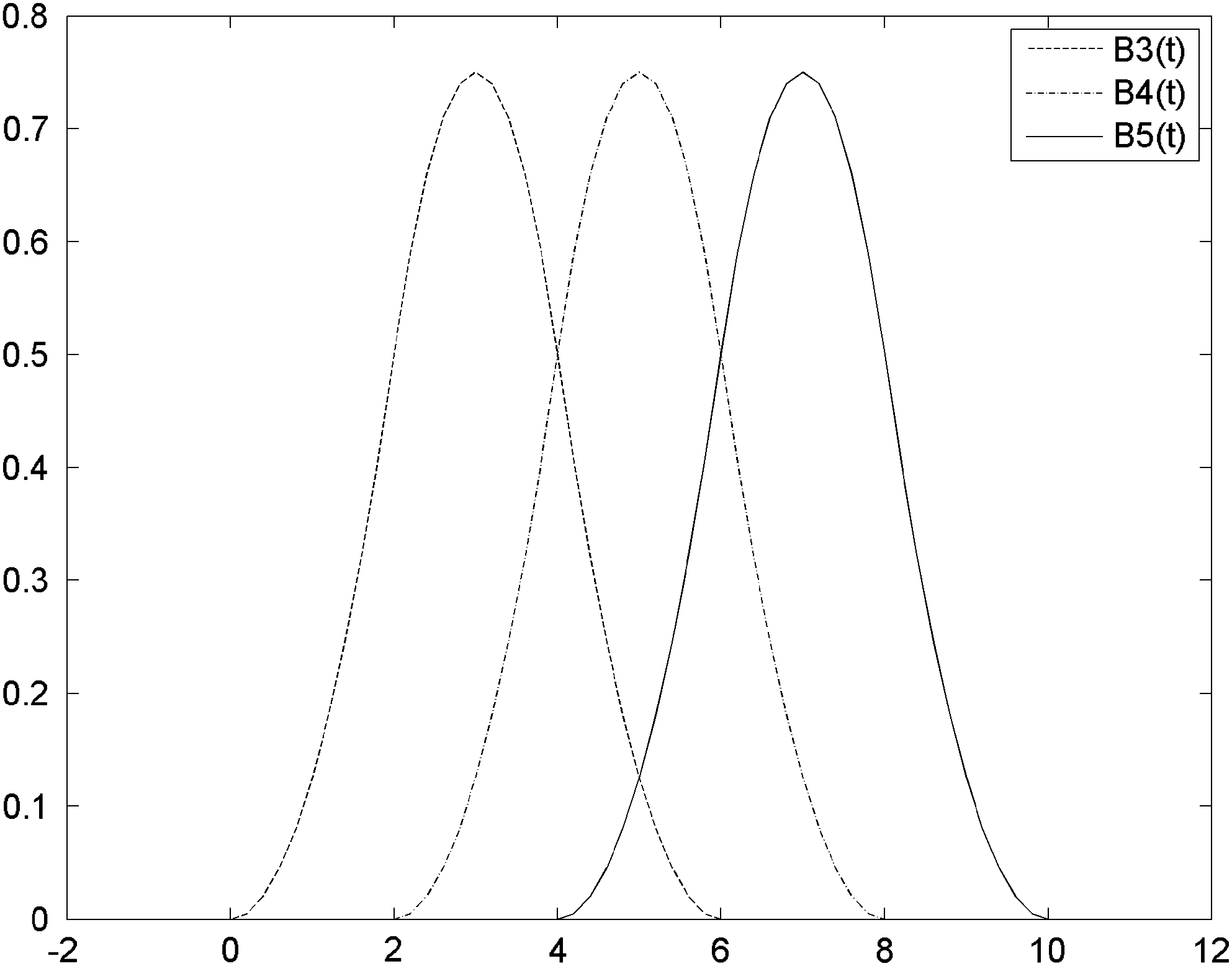
Three quadratic B-spline basis functions.

We used a three-level quadratic B-spline model to model the group-wide, patient-level, and intra-day BG variation.

First, we assume Patient j's BG level at time \documentclass{aastex}\usepackage{amsbsy}\usepackage{amsfonts}\usepackage{amssymb}\usepackage{bm}\usepackage{mathrsfs}\usepackage{pifont}\usepackage{stmaryrd}\usepackage{textcomp}\usepackage{portland,xspace}\usepackage{amsmath,amsxtra}\pagestyle{empty}\DeclareMathSizes{10}{9}{7}{6}\begin{document}$$t \in (0-24) \ {\rm h}$$\end{document} on Day k is BG_jk (t) = f_jk (t) + ɛ_jk (t), where f_jk (t) is a quadratic spline function: \documentclass{aastex}\usepackage{amsbsy}\usepackage{amsfonts}\usepackage{amssymb}\usepackage{bm}\usepackage{mathrsfs}\usepackage{pifont}\usepackage{stmaryrd}\usepackage{textcomp}\usepackage{portland,xspace}\usepackage{amsmath,amsxtra}\pagestyle{empty}\DeclareMathSizes{10}{9}{7}{6}\begin{document}\begin{align*} f_{jk} (t) = \sum_{l = 1}^{14} a_{ljk} B_{l} (t) \tag{1} \end{align*}\end{document}

with basis functions \documentclass{aastex}\usepackage{amsbsy}\usepackage{amsfonts}\usepackage{amssymb}\usepackage{bm}\usepackage{mathrsfs}\usepackage{pifont}\usepackage{stmaryrd}\usepackage{textcomp}\usepackage{portland,xspace}\usepackage{amsmath,amsxtra}\pagestyle{empty}\DeclareMathSizes{10}{9}{7}{6}\begin{document}$$B_{l} (t) , l = 1 , \ldots , 14$$\end{document} and parameters \documentclass{aastex}\usepackage{amsbsy}\usepackage{amsfonts}\usepackage{amssymb}\usepackage{bm}\usepackage{mathrsfs}\usepackage{pifont}\usepackage{stmaryrd}\usepackage{textcomp}\usepackage{portland,xspace}\usepackage{amsmath,amsxtra}\pagestyle{empty}\DeclareMathSizes{10}{9}{7}{6}\begin{document}$$(a_{1 jk} , \ldots , a_{14 jk})$$\end{document} . The 14 basis functions were based on 17 evenly spaced knots at \documentclass{aastex}\usepackage{amsbsy}\usepackage{amsfonts}\usepackage{amssymb}\usepackage{bm}\usepackage{mathrsfs}\usepackage{pifont}\usepackage{stmaryrd}\usepackage{textcomp}\usepackage{portland,xspace}\usepackage{amsmath,amsxtra}\pagestyle{empty}\DeclareMathSizes{10}{9}{7}{6}\begin{document}$$- 4 , - 2 , 0 , 2 , \ldots , 24 , 26 , 28 \ {\rm h}$$\end{document} . The knots at −4 and −2 and at 26 and 28 h were added to aid the computation of basis functions in the (0–4) and (20–24) h intervals, but did not bear physical interpretation. We assumed the errors ɛ_jk (t) were independent and identically distributed (i.i.d.) normally distributed with mean zero and variance σ ².

Next, we assumed that the daily spline coefficients of Patient j were normally distributed around the patient mean with a common covariance matrix, i.e., \documentclass{aastex}\usepackage{amsbsy}\usepackage{amsfonts}\usepackage{amssymb}\usepackage{bm}\usepackage{mathrsfs}\usepackage{pifont}\usepackage{stmaryrd}\usepackage{textcomp}\usepackage{portland,xspace}\usepackage{amsmath,amsxtra}\pagestyle{empty}\DeclareMathSizes{10}{9}{7}{6}\begin{document}\begin{align*}(a_{1 jk} , \ldots , a_{14 jk}) \sim {\rm Normal} \ ((a_{1j} , \ldots , a_{14 j}) , {\it \Phi}) \tag{2} \end{align*}\end{document}

Using this structure, we modeled that Patient j's daily glucose trends vary around a mean trend function (i.e., a patient-level profile) of \documentclass{aastex}\usepackage{amsbsy}\usepackage{amsfonts}\usepackage{amssymb}\usepackage{bm}\usepackage{mathrsfs}\usepackage{pifont}\usepackage{stmaryrd}\usepackage{textcomp}\usepackage{portland,xspace}\usepackage{amsmath,amsxtra}\pagestyle{empty}\DeclareMathSizes{10}{9}{7}{6}\begin{document}$$f_{j} (t) = \sum \nolimits_{l = 1}^{14} a_{lj} B_{l} (t)$$\end{document} . We assumed that all within-patient, inter-day covariance matrices were the same (Φ). If necessary and computationally feasible, this assumption can be relaxed to allow the variance matrix to vary with patient.

Finally, we assumed that the patient-specific parameters were normally distributed around a group-wide mean with covariance matrix Σ, \documentclass{aastex}\usepackage{amsbsy}\usepackage{amsfonts}\usepackage{amssymb}\usepackage{bm}\usepackage{mathrsfs}\usepackage{pifont}\usepackage{stmaryrd}\usepackage{textcomp}\usepackage{portland,xspace}\usepackage{amsmath,amsxtra}\pagestyle{empty}\DeclareMathSizes{10}{9}{7}{6}\begin{document}\begin{align*}(a_{1j} , \ldots , a_{14j}) \sim {\rm Normal} \ ((a_{1} , \ldots , a_{14}) , \Sigma) \tag{3} \end{align*}\end{document}

This structure assumes that patient-specific trend functions vary around a group-wide trend function (i.e., a group-wide profile): \documentclass{aastex}\usepackage{amsbsy}\usepackage{amsfonts}\usepackage{amssymb}\usepackage{bm}\usepackage{mathrsfs}\usepackage{pifont}\usepackage{stmaryrd}\usepackage{textcomp}\usepackage{portland,xspace}\usepackage{amsmath,amsxtra}\pagestyle{empty}\DeclareMathSizes{10}{9}{7}{6}\begin{document}\begin{align*} f (t) = \sum_{l = 1}^{14} a_{l} B_{l} (t) \end{align*}\end{document}

At a typical time point, three consecutive quadratic B-spline basis functions take non-zero values, suggesting that the adjacent parameters are correlated with \documentclass{aastex}\usepackage{amsbsy}\usepackage{amsfonts}\usepackage{amssymb}\usepackage{bm}\usepackage{mathrsfs}\usepackage{pifont}\usepackage{stmaryrd}\usepackage{textcomp}\usepackage{portland,xspace}\usepackage{amsmath,amsxtra}\pagestyle{empty}\DeclareMathSizes{10}{9}{7}{6}\begin{document}$$(a_{{l_1} jk} , . a_{{l_2} jk}) \neq 0$$\end{document} for any ∣l ₁ − l ₂∣ ≤ 2. An examination of the unrestricted autocorrelation functions revealed a banded covariance structure for the intra-day glucose curve (Fig. 2A) and an unstructured covariance matrix for patient-level curve (Fig. 2B). Numerical comparisons showed that unstructured and banded Toeplitz within-patient inter-day Φ matrices^12
–14 lead to very similar estimations for individual and group-wide profiles. We used a Toeplitz (3) structure as the within-patient inter-day covariance Φ for its efficiency in computer memory and CPU time usage without sacrificing numerical accuracy.

FIG. 2.

Autocorrelation of (A) the daily glucose curve and (B) the patient average glucose profile for type 1 diabetes. The z-axis represents the correlation coefficient between glucose values at a time point on the x-axis and a time point on the y-axis. The time unit is h.

This model can be parameterized as a linear mixed effects model^15
–17 and fitted using conventional statistical software such as SAS version 9.2 (SAS Institute, Inc., Cary, NC). In SAS PROC MIXED, this model requires two “random” statements to specify the patient-level and within-patient, day-to-day random effects. Some sample SAS code is given in Appendix B.

One can view the proposed model as a hierarchical Bayesian model with normal priors for the B-spline coefficients and use Bayesian algorithms to draw inferences.

Model-based variance estimation of the glucose profiles

Using the proposed hierarchical model, we were able to estimate the inter-patient and inter-day covariance matrices of model coefficients and calculate the point-wise variance of the mean glucose functions.

The inter-patient variance of BG function at time point t was given by \documentclass{aastex}\usepackage{amsbsy}\usepackage{amsfonts}\usepackage{amssymb}\usepackage{bm}\usepackage{mathrsfs}\usepackage{pifont}\usepackage{stmaryrd}\usepackage{textcomp}\usepackage{portland,xspace}\usepackage{amsmath,amsxtra}\pagestyle{empty}\DeclareMathSizes{10}{9}{7}{6}\begin{document}\begin{align*} Var (f_j (t)) = Var \Big(\sum_{l = 1}^{14} a_{lj} B_{l} (t) \Big)= B (t)^{T} \Sigma B (t) \tag{4} \end{align*}\end{document}

where B(t) is the 14 × 1 matrix containing the values \documentclass{aastex}\usepackage{amsbsy}\usepackage{amsfonts}\usepackage{amssymb}\usepackage{bm}\usepackage{mathrsfs}\usepackage{pifont}\usepackage{stmaryrd}\usepackage{textcomp}\usepackage{portland,xspace}\usepackage{amsmath,amsxtra}\pagestyle{empty}\DeclareMathSizes{10}{9}{7}{6}\begin{document}$$B_1 (t) , \ldots , B_{14} (t)$$\end{document} .

Similarly, for Patient j, the inter-day variation of BG function at time point t was given by \documentclass{aastex}\usepackage{amsbsy}\usepackage{amsfonts}\usepackage{amssymb}\usepackage{bm}\usepackage{mathrsfs}\usepackage{pifont}\usepackage{stmaryrd}\usepackage{textcomp}\usepackage{portland,xspace}\usepackage{amsmath,amsxtra}\pagestyle{empty}\DeclareMathSizes{10}{9}{7}{6}\begin{document}\begin{align*} Var (f_{jk} (t) | j) = Var \Big(\sum_{l = 1}^{14} a_{ljk} B_l (t) \Big) = B (t)^{T} {\it \Phi} B (t) \tag{5} \end{align*}\end{document}

The above two quantities were estimated by replacing \documentclass{aastex}\usepackage{amsbsy}\usepackage{amsfonts}\usepackage{amssymb}\usepackage{bm}\usepackage{mathrsfs}\usepackage{pifont}\usepackage{stmaryrd}\usepackage{textcomp}\usepackage{portland,xspace}\usepackage{amsmath,amsxtra}\pagestyle{empty}\DeclareMathSizes{10}{9}{7}{6}\begin{document}$${\it \Sigma}$$\end{document} and \documentclass{aastex}\usepackage{amsbsy}\usepackage{amsfonts}\usepackage{amssymb}\usepackage{bm}\usepackage{mathrsfs}\usepackage{pifont}\usepackage{stmaryrd}\usepackage{textcomp}\usepackage{portland,xspace}\usepackage{amsmath,amsxtra}\pagestyle{empty}\DeclareMathSizes{10}{9}{7}{6}\begin{document}$${\it \Phi}$$\end{document} by their maximum likelihood (ML) or restricted maximum likelihood (REML) estimates, \documentclass{aastex}\usepackage{amsbsy}\usepackage{amsfonts}\usepackage{amssymb}\usepackage{bm}\usepackage{mathrsfs}\usepackage{pifont}\usepackage{stmaryrd}\usepackage{textcomp}\usepackage{portland,xspace}\usepackage{amsmath,amsxtra}\pagestyle{empty}\DeclareMathSizes{10}{9}{7}{6}\begin{document}$${\it \hat{\Sigma}}$$\end{document} and \documentclass{aastex}\usepackage{amsbsy}\usepackage{amsfonts}\usepackage{amssymb}\usepackage{bm}\usepackage{mathrsfs}\usepackage{pifont}\usepackage{stmaryrd}\usepackage{textcomp}\usepackage{portland,xspace}\usepackage{amsmath,amsxtra}\pagestyle{empty}\DeclareMathSizes{10}{9}{7}{6}\begin{document}$$\hat {\Phi}$$\end{document} , respectively.

The SE of the group-wide function and patient-specific mean function can be estimated by replacing the variance–covariance matrices in the above equations by the estimated variance–covariance matrices of \documentclass{aastex}\usepackage{amsbsy}\usepackage{amsfonts}\usepackage{amssymb}\usepackage{bm}\usepackage{mathrsfs}\usepackage{pifont}\usepackage{stmaryrd}\usepackage{textcomp}\usepackage{portland,xspace}\usepackage{amsmath,amsxtra}\pagestyle{empty}\DeclareMathSizes{10}{9}{7}{6}\begin{document}$$(\hat{a}_{1j} , \ldots , \hat{a}_{14j})$$\end{document} and \documentclass{aastex}\usepackage{amsbsy}\usepackage{amsfonts}\usepackage{amssymb}\usepackage{bm}\usepackage{mathrsfs}\usepackage{pifont}\usepackage{stmaryrd}\usepackage{textcomp}\usepackage{portland,xspace}\usepackage{amsmath,amsxtra}\pagestyle{empty}\DeclareMathSizes{10}{9}{7}{6}\begin{document}$$(\hat{a}_{1jk} , \ldots , \hat{a}_{14jk})$$\end{document} , respectively.

The matrices \documentclass{aastex}\usepackage{amsbsy}\usepackage{amsfonts}\usepackage{amssymb}\usepackage{bm}\usepackage{mathrsfs}\usepackage{pifont}\usepackage{stmaryrd}\usepackage{textcomp}\usepackage{portland,xspace}\usepackage{amsmath,amsxtra}\pagestyle{empty}\DeclareMathSizes{10}{9}{7}{6}\begin{document}$${\it \hat {\Sigma}}$$\end{document} and \documentclass{aastex}\usepackage{amsbsy}\usepackage{amsfonts}\usepackage{amssymb}\usepackage{bm}\usepackage{mathrsfs}\usepackage{pifont}\usepackage{stmaryrd}\usepackage{textcomp}\usepackage{portland,xspace}\usepackage{amsmath,amsxtra}\pagestyle{empty}\DeclareMathSizes{10}{9}{7}{6}\begin{document}$${\it \hat {\Phi}}$$\end{document} , the covariance matrices of \documentclass{aastex}\usepackage{amsbsy}\usepackage{amsfonts}\usepackage{amssymb}\usepackage{bm}\usepackage{mathrsfs}\usepackage{pifont}\usepackage{stmaryrd}\usepackage{textcomp}\usepackage{portland,xspace}\usepackage{amsmath,amsxtra}\pagestyle{empty}\DeclareMathSizes{10}{9}{7}{6}\begin{document}$$(\hat{a}_{1j} , \ldots , \hat{a}_{14j})$$\end{document} and \documentclass{aastex}\usepackage{amsbsy}\usepackage{amsfonts}\usepackage{amssymb}\usepackage{bm}\usepackage{mathrsfs}\usepackage{pifont}\usepackage{stmaryrd}\usepackage{textcomp}\usepackage{portland,xspace}\usepackage{amsmath,amsxtra}\pagestyle{empty}\DeclareMathSizes{10}{9}{7}{6}\begin{document}$$(\hat{a}_{1jk} , \ldots , \hat{a}_{14jk})$$\end{document} , and the error variance σ ² can all be estimated under the mixed effects model theory.

Validation of the model-based SE estimation

The aforementioned model-based variance estimation requires fairly accurate estimation of the variance–covariance matrices. A robust, but computationally intensive, alternative is the replication-based method, which does not involve the estimation of covariance matrices. We used a replication-based method to verify the model-based estimation.

We applied the following bootstrap method to estimate the SE of group-wide profiles. We created 10 replication samples by drawing with replacement from the sample the same number of patients. We applied the three-level model to each replication sample to obtain a replicate estimate of the mean glucose trend function. From the replicate estimates, we calculated the bootstrap estimate of the point-wise SE of the mean trend function. To check the validity of the model-based SE, we compared the bootstrap variance estimation with the model-based estimation on the type 1 diabetes patients' data.

Comparison of glucose profiles between patient groups

In order to demonstrate the utility of the proposed model in comparing BG profiles, we compared two groups of type 1 diabetes patients: group 1 was insulin pump–treated, and group 2 was treated with multiple daily injection (MDI) therapy. The goal was to assess how much, on average, the use of an insulin pump influenced the glucose profile in type 1 diabetes. In order to perform this exemplary comparison, we defined a group indicator I_j which was 0 if Patient j was in group 1 and 1 if the patient was in group 2.

We introduced 14 additional parameters \documentclass{aastex}\usepackage{amsbsy}\usepackage{amsfonts}\usepackage{amssymb}\usepackage{bm}\usepackage{mathrsfs}\usepackage{pifont}\usepackage{stmaryrd}\usepackage{textcomp}\usepackage{portland,xspace}\usepackage{amsmath,amsxtra}\pagestyle{empty}\DeclareMathSizes{10}{9}{7}{6}\begin{document}$$({\it \Delta}_1 , \ldots , {\it \Delta}_{14})$$\end{document} that represented the differences in spline coefficients between group 2 and group 1. The group model (3) was then modified to be \documentclass{aastex}\usepackage{amsbsy}\usepackage{amsfonts}\usepackage{amssymb}\usepackage{bm}\usepackage{mathrsfs}\usepackage{pifont}\usepackage{stmaryrd}\usepackage{textcomp}\usepackage{portland,xspace}\usepackage{amsmath,amsxtra}\pagestyle{empty}\DeclareMathSizes{10}{9}{7}{6}\begin{document}$$(a_{1j} , \ldots , a_{14j}) \sim {\rm Normal} \ ((a_{1} + {\it \Delta}_1 I_j , \ldots , a_{14} + {\it \Delta}_{14} I_j) , {\it \Sigma})$$\end{document} so that group 1 and group 2 were modeled to have different profiles. In the mixed effects model, parameters \documentclass{aastex}\usepackage{amsbsy}\usepackage{amsfonts}\usepackage{amssymb}\usepackage{bm}\usepackage{mathrsfs}\usepackage{pifont}\usepackage{stmaryrd}\usepackage{textcomp}\usepackage{portland,xspace}\usepackage{amsmath,amsxtra}\pagestyle{empty}\DeclareMathSizes{10}{9}{7}{6}\begin{document}$$({\it \Delta}_1 , \ldots , {\it \Delta}_{14})$$\end{document} were treated as fixed effects. One can use the Hotelling T-square test¹⁸ for the null hypothesis that \documentclass{aastex}\usepackage{amsbsy}\usepackage{amsfonts}\usepackage{amssymb}\usepackage{bm}\usepackage{mathrsfs}\usepackage{pifont}\usepackage{stmaryrd}\usepackage{textcomp}\usepackage{portland,xspace}\usepackage{amsmath,amsxtra}\pagestyle{empty}\DeclareMathSizes{10}{9}{7}{6}\begin{document}$${\it \Delta}_1 = {\it \Delta}_2 = \ldots = {\it \Delta}_{14} = 0$$\end{document} . One can use the Bayesian model to allow either identical or different covariance matrices in the comparison groups. For pump versus MDI comparison, we assume the two groups have the same covariance matrices.

The difference of the two spline functions is still a spline function with parameters \documentclass{aastex}\usepackage{amsbsy}\usepackage{amsfonts}\usepackage{amssymb}\usepackage{bm}\usepackage{mathrsfs}\usepackage{pifont}\usepackage{stmaryrd}\usepackage{textcomp}\usepackage{portland,xspace}\usepackage{amsmath,amsxtra}\pagestyle{empty}\DeclareMathSizes{10}{9}{7}{6}\begin{document}$$({\it \Delta}_1 , \ldots , {\it \Delta}_{14})$$\end{document} . The estimates \documentclass{aastex}\usepackage{amsbsy}\usepackage{amsfonts}\usepackage{amssymb}\usepackage{bm}\usepackage{mathrsfs}\usepackage{pifont}\usepackage{stmaryrd}\usepackage{textcomp}\usepackage{portland,xspace}\usepackage{amsmath,amsxtra}\pagestyle{empty}\DeclareMathSizes{10}{9}{7}{6}\begin{document}$$(\hat {\it \Delta}_1 , \ldots , \hat {\it \Delta}_{14})$$\end{document} and their covariance matrix are useful for making various comparisons. Point-wise estimates and credible intervals (CI) (Bayesian language for confidence interval) of the difference between the two profiles can be obtained at any time point. The difference can be plotted versus time in the form of a spline function (D-curve) and its CI. From the 95% CI of the D-curve one can identify time periods in which two profiles are significantly different.

The area under the curve (AUC) values of two group-wide trend functions can also be compared. This requires the calculation of AUC for each basis function, which equals \documentclass{aastex}\usepackage{amsbsy}\usepackage{amsfonts}\usepackage{amssymb}\usepackage{bm}\usepackage{mathrsfs}\usepackage{pifont}\usepackage{stmaryrd}\usepackage{textcomp}\usepackage{portland,xspace}\usepackage{amsmath,amsxtra}\pagestyle{empty}\DeclareMathSizes{10}{9}{7}{6}\begin{document}$$\frac {1} {3}$$\end{document} for B ₁ (t) and B ₁₄ (t), \documentclass{aastex}\usepackage{amsbsy}\usepackage{amsfonts}\usepackage{amssymb}\usepackage{bm}\usepackage{mathrsfs}\usepackage{pifont}\usepackage{stmaryrd}\usepackage{textcomp}\usepackage{portland,xspace}\usepackage{amsmath,amsxtra}\pagestyle{empty}\DeclareMathSizes{10}{9}{7}{6}\begin{document}$$\frac {5} {3}$$\end{document} for B ₂ (t) and B ₁₃ (t), and 2 for B ₃ (t) to B ₁₂ (t).

Comparisons of nonlinear quantities such as maximum and minimum differences are possible using simulations. One can draw from the joint posterior distribution of \documentclass{aastex}\usepackage{amsbsy}\usepackage{amsfonts}\usepackage{amssymb}\usepackage{bm}\usepackage{mathrsfs}\usepackage{pifont}\usepackage{stmaryrd}\usepackage{textcomp}\usepackage{portland,xspace}\usepackage{amsmath,amsxtra}\pagestyle{empty}\DeclareMathSizes{10}{9}{7}{6}\begin{document}$$({\it \Delta}_1 , \ldots , {\it \Delta}_{14})$$\end{document} and obtain distributions of such quantities for statistical inference.

Results

We analyzed CGM data from three groups of patients separately using the proposed model: 322 patients with type 1 diabetes, 223 patients with type 2 diabetes, and 86 subjects without diabetes. Among the type 1 diabetes patients for whom treatment was consistent during the study, 124 were treated with an insulin pump, and 144 were treated with MDI. The median age of the patients was 45 years (range, 16–70 years), and 53% were female. The characteristics of the study group are shown in Table 1.

Table 1.

Baseline Characteristics of the Study Cohort

	Type 1 diabetes
	Overall ^*	Pump-treated	MDI-treated	Type 2 diabetes	Without diabetes
Number	322	124	144	223	86
Age (mean ± SD) (years)	43 ± 13	43 ± 13	44 ± 13	55 ± 9	40 ± 14
Number (%) of females	166 (52%)	70 (57%)	70 (49%)	111 (50%)	59 (69%)
HbA1c (mean ± SD) (%)	7.3 ± 1.2	7.2 ± 1.1	7.4 ± 1.2	6.8 ± 1.1	5.2 ± 0.3

Includes patients whose treatment information was not available or not determined.

HbA1c, hemoglobin A1c.

Using the three-level spline model, we were able to obtain patient-specific and group-wide glucose functions for type 1 and type 2 diabetes and for the subjects without diabetes. We were also able to estimate the 95% CI for each diabetes type.

Table 2 gives the 24-h average inter-day and inter-patient variations in the three groups: type 1 diabetes, type 2 diabetes, and subjects without diabetes. Type 1 and type 2 diabetes patients had similar inter-patient variability with an average SD of approximately 49 and 43 mg/dL, respectively, compared with 15 mg/dL for the subjects without diabetes. Type 1 diabetes patients showed higher inter-day variability than type 2 patients (SD = 67 vs. 41 mg/dL, P < 0.001 according to the estimated asymptotic distribution of the covariance parameters). Type 1 diabetes patients' inter-day variability was higher than their inter-patient variability (SD = 67 vs. 49 mg/dL). Type 1 diabetes had the highest residual SD of 19 mg/dL versus 14 mg/dL for type 2 diabetes and 8 mg/dL for subjects without diabetes.

Table 2.

Average Inter-Patient and Within-Patient, Inter-Day SD of Blood Glucose Profile by Group

	Average SD (mg/dL)
	Inter-patient	Inter-day	Residual
Type 1 diabetes	49	67	19
Type 2 diabetes	43	41	14
Without diabetes	15	18	8

The model-based SE estimate was close to the bootstrap estimates for type 1 diabetes patients. The 24-h average model-based SE estimate was 3.1 mg/dL, which is close to the bootstrap estimate of 2.9 mg/dL.

The quadratic B-spline model leads to smooth curves tightly tracking the individual patient's CGM measurements. Figure 3 demonstrates the smoothed intra-day BG curve, and its 95% CI overlapped with the measured BG of a type 1 diabetes patient over a 24-h period.

FIG. 3.

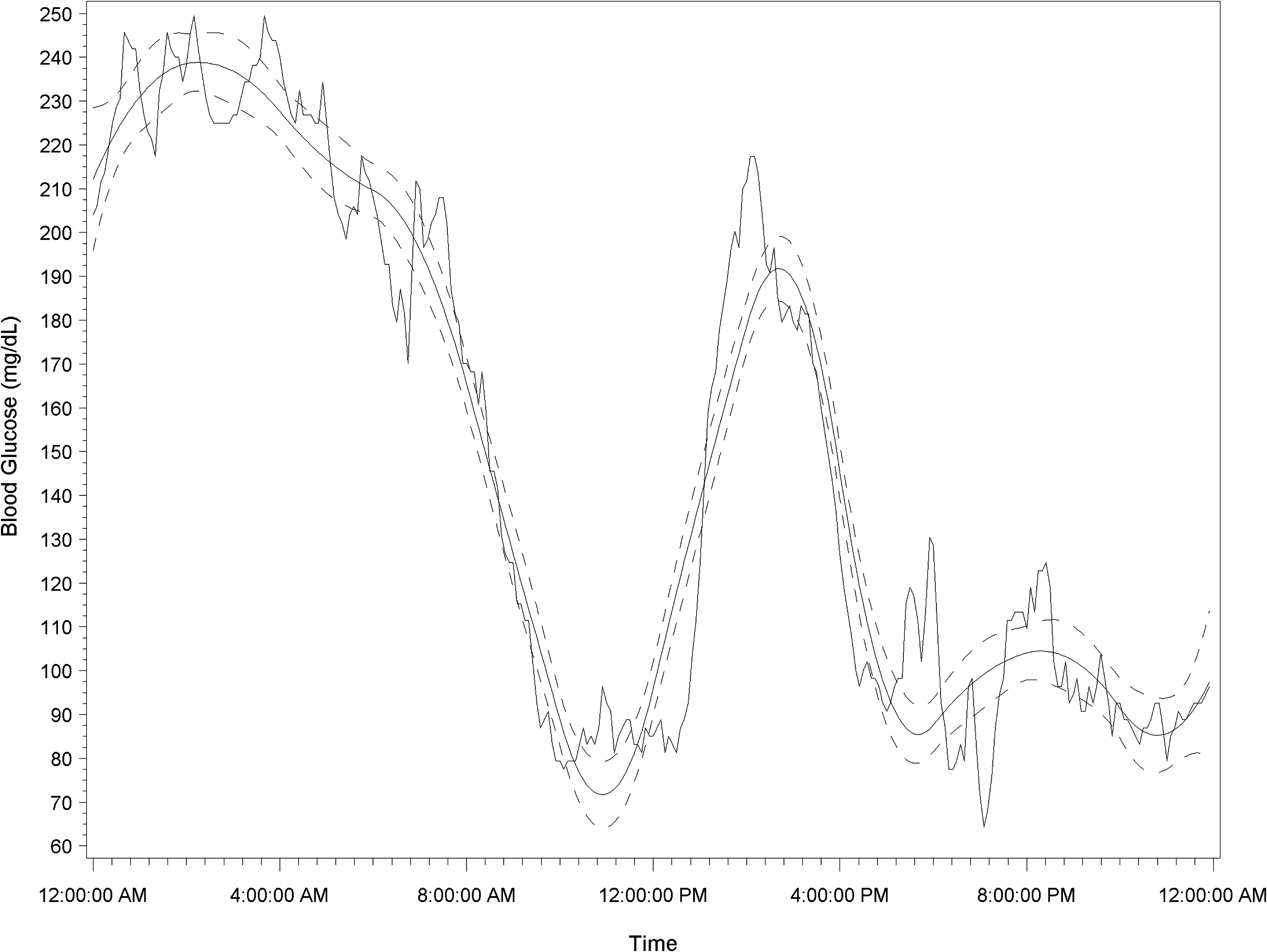
Blood glucose curve and 95% credible interval (dashed lines) overlapped with the continuous glucose monitoring measurement of a type 1 diabetes patient over a 24-h period.

Figure 4A shows the group-wide 24-h glucose profile for type 1 diabetes patients treated with an insulin pump. The group-wide glucose curve of such patients trended within the 145–180 mg/dL range and had peaks at three time points: at approximately 9 a.m., 3 p.m., and midnight, corresponding to the effects of three meals. By comparison, the group-wide 24-h glucose curves for type 1 diabetes patients treated with MDI trended within the 145–190 mg/dL range and peaked at approximately 9–10 a.m. and midnight (Fig. 4B).

FIG. 4.

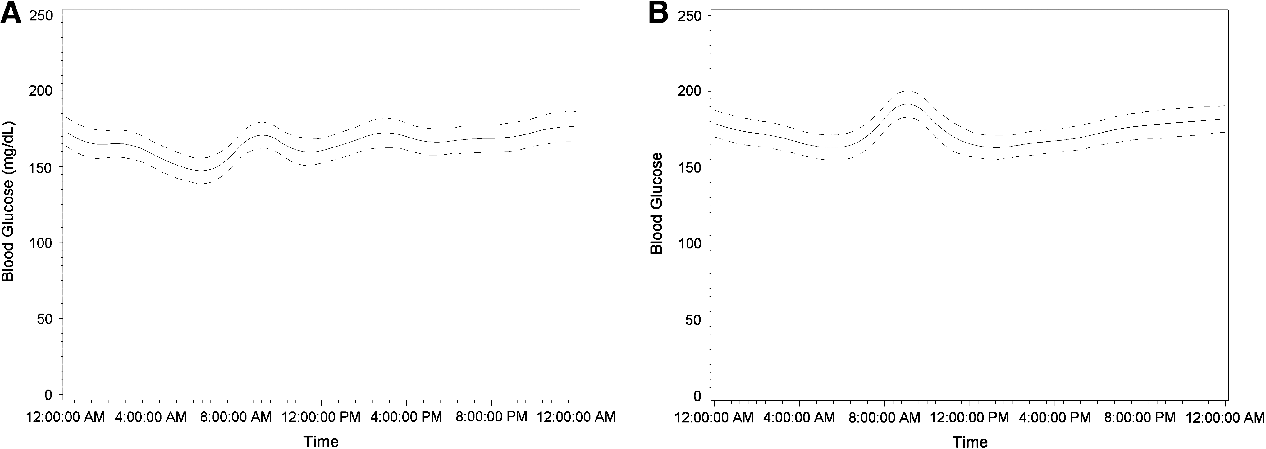
Group-wide blood glucose curve and 95% credible interval (dashed lines) of type 1 diabetes patients treated with (A) an insulin pump and (B) multiple daily injections.

Figure 5 illustrates the estimated difference between MDI-treated and pump-treated type 1 diabetes patients' glucose profiles and the 95% CI of the differences. Figure 5 shows that glucose levels of MDI-treated patients are significantly higher than those of pump-treated patients from around 6 a.m. to around 10 a.m. The Hotelling¹⁸ T-square test for the equality of the two group level profiles leads to a P value of 0.14, suggesting no significant difference between the two group-wide profiles as a whole.

FIG. 5.

Estimated mean and 95% credible interval (dashed lines) of the difference in glucose profiles between multiple daily injection–treated and insulin pump–treated type 1 diabetes patients. Higher values represent higher values in multiple daily injection–treated compared with insulin pump–treated patients.

Discussion

The three-level B-spline model provides a framework for the smoothing and inference of the dense glucose data provided by CGM. The model allows us to estimate the patient-level and group-level glucose profiles and their variability, as well as to make statistical comparisons of profiles among different groups.

The model yields smooth curves tightly tracking the CGM measurements. Not surprisingly, the population mean glucose profiles reflect the well-recognized effects of eating on glycemic excursions. The model provides insights into the different patterns of glycemia achieved with therapy in type 1 diabetes and, potentially, the timing and types of interventions necessary to address the glucose excursions.

The evenly spaced knots are a natural fit for the CGM measurements by including the same number of measurements in each time interval between consecutive knots. Statistical criteria for selection of number and placement of knots have been widely discussed. Such methods include Akaike information criterion, Bayesian information criterion, cross-validation, and Bayesian model selection methods such as the reversible jump Markov chain Monte Carlo method.¹⁹ In practice, the choice of knots should be based on a combination of statistical and practical considerations. In a situation where more detailed examination of the glucose curve is necessary, a larger number of knots can be used.

The choice of covariance structures has a limited impact on the estimated shapes of trend functions. Mis-specified covariance structures still lead to unbiased, albeit not the most efficient, estimates of the glucose curves. However, the covariance structures play an important role in variance estimation and hypothesis testing. This model assumes i.i.d. Gaussian random errors with mean zero and does not account for correlations among measurement errors.

Although the replication-based method provides robust variance estimation, it is computationally resource-demanding, making it infeasible for large datasets. In contrast, the model-based method is computationally efficient for large datasets without sacrificing the quality of variance estimation.

The proposed model allows statistical comparisons of point-wise and overall differences between two (or more) profiles, thus providing a useful statistical tool for future clinical trials using glucose profiles as an endpoint. Power calculations for such statistical tests are possible using estimated variance components and the expected effect size.

The B-spline basis functions demonstrated a numerical advantage in variance estimation over an alternative, the truncated polynomial functions. B-splines lead to more sparse and well-conditioned covariance matrices, whereas truncated polynomials are more prone to yield unsatisfactory variance estimation.

For large samples, the three-level random effects model is resource-demanding in terms of computer memory and CPU time. It would have been impossible to fit such a model on the ADAG data using a regular PC a few years ago. However, with the computational power of today's personal computers, such models can be fitted on sizeable samples in a reasonable amount of time using a common PC.

This model could be used in software to help patients better control their glucose. The mathematical methods for this are beyond the scope of this article, but they would involve using variance covariance matrix as part of a prior distribution for the individual parameters that define a patient's daily profile. Then the patient's daily profile can be estimated from several weeks of data. This profile, along with a record of insulin injections, food intake, and exercise, can be used to determine behavior changes that might improve the patient's glucose control. We contemplate clinical trials comparing such a strategy to other treatment strategies. The methods we propose could also help improve estimation of instantaneous insulin values by using the model parameters in a prior distribution for each reading. This would involve building software into the device.

The B-splines-based Bayesian modeling techniques provide a promising tool for clinical decision-making and ultimately for the development of “closed-loop” systems.

Footnotes

Acknowledgments

Support for the current analyses was provided by the Charlton Fund for Innovative Diabetes Research at Massachusetts General Hospital and from Harvard Catalyst, The Harvard Clinical and Translational Science Center (National Institutes of Health Award number UL1 RR 025758 and financial contributions from Harvard University and its affiliated academic health care centers). ADAG was supported by research grants from the American Diabetes Association (7-06-A1C-11) and the European Association for the Study of Diabetes. Financial support for ADAG was provided by Abbott Diabetes Care, Bayer Healthcare, GlaxoSmithKline, Sanofi-Aventis Netherlands, Merck & Company, Lifescan, Inc., and Medtronic MiniMed, and supplies and equipment were provided by Medtronic MiniMed, Lifescan, Inc., and Hemocue. A complete listing of the ADAG Research Group can be found in Nathan et al.⁹ The content is solely the responsibility of the authors and does not necessarily represent the official views of Harvard Catalyst, Harvard University and its affiliated academic health care centers, the National Center for Research Resources, the National Institutes of Health, or the ADAG Research Group.

Author Disclosure Statement

None of the authors has a conflict of interest regarding the submitted manuscript.

Appendix A

Appendix B

References

Deiss

, Bolinder

, Riveline

, Battelino

, Bosi

, Tubiana-Rufi

, Kerr

, Phillip

. Improved glycemic control in poorly controlled patients with type 1 diabetes using real-time continuous glucose monitoring. Diabetes Care, 2006; 29:2730–2732.

Tamborlane

, Beck

, Bode

, Buckingham

, Chase

, Clemons

, Fiallo-Scharer

, Fox

, Gilliam

, Hirsch

, Huang

, Kollman

, Kowalski

, Laffel

, Lawrence

, Lee

, Mauras

, O'Grady

, Ruedy

, Tansey

, Tsalikian

, Weinzimer

, Wilson

, Wolpert

, Wysocki

, Xing

. Continuous glucose monitoring and intensive treatment of type 1 diabetes. N Engl J Med, 2008; 359:1464–1476.

Tamborlane

, Beck

. Continuous glucose monitoring in type 1 diabetes mellitus. Lancet, 2009; 373:1744–1746.

Boyne

, Silver

, Kaplan

, Saudek

. Timing of changes in interstitial and venous blood glucose measured with a continuous subcutaneous glucose sensor. Diabetes, 2003; 52:2790–2794.

Eilers

, Marx

. Flexible Smoothing with B-splines and penalties. Stat Sci, 1996; 11:89–121.

Ruppert

, Carroll

. Spatially adaptive penalties for spline fitting. Aust N Z J Stat, 2000; 42:205–223.

Rice

, Wu

. Nonparametric mixed effects models for unequally sampled noisy curves. Biometrics, 2001; 57:253–259.

Mazze

, Strock

, Borgman

, Wesley

, Stout

, Racchini

. Evaluating the accuracy, reliability, and clinical applicability of continuous glucose monitoring (CGM): is CGM ready for real time? Diabetes Technol Ther, 2009; 11:11–18.

Nathan

, Kuenen

, Borg

, Zheng

, Schoenfeld

, Heine

. Translating the A1C assay into estimated average glucose values. Diabetes Care, 2008; 31:1473–1478.

10.

De Boor

. Package for calculating with B-splines. SIAM J Numerical Anal, 1977; 14:441–472.

11.

De Boor

. A Practical Guide to Splines. Berlin: Springer, 1978.

12.

Grenander

, Szegö

. Toeplitz Forms and Their Applications. Berkeley and Los Angeles: University of California Press, 1958.

13.

Widom

. Toeplitz matrices. Hirschmann

Jr . MAA Studies in Mathematics: Studies in Real and Complex Analysis. Englewood Cliffs, NJ: Prentice-Hall, 1965; 179–209.

14.

Böttcher

, Silbermann

. Introduction to Large Truncated Toeplitz Matrices. New York: Springer, 1999.

15.

Laird

, Ware

. Random-effects models for longitudinal data. Biometrics, 1982; 38:963–974.

16.

Raudenbush

, Bryk

. Hierarchical Linear Models: Applications, Data Analysis Methods. Thousand Oaks, CA: Sage, 2002.

17.

Singer

. Using SAS PROC MIXED to fit multilevel models, hierarchical models, and individual growth models. J Educ Behav Stat, 1998; 24:323–355.

18.

Hotelling

. The generalization of Student's ratio. Ann Math Stat, 1931; 2:360–378.

19.

Green

. Reversible jump Markov chain Monte Carlo computation and Bayesian model determination. Biometrika, 1995; 82:711–732.